i
Geometric Parameterisation and
Aerodynamic Shape Optimisation
Name: Feng Zhu
Supervisor: Prof Ning Qin
Email: [email protected]
Address: Department of Mechanical Engineering
University of Sheffield
S1 3JD
i
Abstract
Aerodynamic optimisation plays an increasingly important role in the aircraft industry. In aerodynamic optimisation, shape parameterisation is the key technique, since it determines the design space. The ideal parameterisation method should be able to provide a high level of flexibility with a low number of design variables to reduce the complexity of the design space. In this work, the Class/Shape Function Transformation (CST) method is investigated for geometric representation of an entire transport aircraft for the purpose of aerodynamic optimisation. It is then further developed for an entire passenger transport aircraft, including such components as the wing, horizontal tail plane, vertical tail plane, fuselage, belly fairing, wingtip device, nacelle, flap tracking fairing and pylon. This work presents the parameterisation of these components in detail using the CST methods for the reference of future aerodynamic optimisation work. The intersection line calculation method between CST components is presented for future entire aircraft optimisation. The performance of the CST has been tested as well, and it found a few drawbacks of the CST methods; for example, it cannot provide some key intuitive design parameters and can lose the accuracy in the wing leading edge area. Therefore, two derivatives of the CST method are proposed: one is called the intuitive CST method (iCST), which is to transform the CST parameters to intuitive design parameters; the other is called the RCST method, which is able to increase the fitting accuracy of the original CST method with fewer design variables. Their performances are studied by comparing them regarding their accuracy in inversely fitting a wide range of aerofoils. Finally, the CST method is also developed to represent the shock control bump, which has better curvature continuity than cubic polynomials.
The aerodynamic optimisation study based on adjoint approaches is carried out using the above parameterisation methods. Optimisation was performed on two-dimensional cases to make a preliminary investigation of the performances of the above parameterisation methods. The results showed that all of CST, iCST and RCST parameterisation methods are able to successfully reduce the drag. The results of the CST methods showed the
ii lower order CST is able to provide fast convergence, and the high order CST is able to provide more flexibility and more local control of the shape to reach better optimal solution. The iCST providing intuitive parameters is improving the process of setup constraints, which is useful for aerofoil optimisation. The RCST showed good performance in aerodynamic optimisation in terms of convergence rate, number of design variables, low order of polynomials and smoothness of the shape. This work provides a reference to designer for choosing suitable parameterisation method in these three methods regarding specific requirement. The shock control bump optimisation on 2D aerofoil is performed to compare three shock control bump parameterisation methods. The results showed the CST parameterisation method is promising for shock control bump optimisation.
Three-dimensional optimisation tests, including wing and winglet drag minimisation, were performed using the above parameterisation methods. The results showed that the CST methods are able to handle three-dimensional wing optimisation. It also investigated the effect of the order of CST method in optimisation. The results showed the lower order CST already performed well in optimisation in terms of optimal results and convergence rate. The optimisation also discussed the importance of using Cmx constraint in aerodynamic optimisation. In the winglet test cases, it showed the CST methods and adjoint approach are able to perform winglet optimisation. The drag of four winglets are successfully reduced. The downward winglet showed the potential benefits in terms of lower wing root bending momentum. At the end, the shock control bump optimisation using CST method on 3D wing has been performed. The results showed the mesh adjoint methods is able to identify the sensitive area for deploying shock control bumps and the CST shock control bump successfully reduced the wave drag.
iii
Acknowledgements
I sincerely appreciate my supervisor Prof. Ning Qin for his guidance. He offered me this opportunity and led me into a very interesting aerodynamic design and optimisation area, and has provided me with endless helpful advice to overcome all difficulties throughout the years. I also would like to thank present and former colleagues in the Aerodynamics Group at the University of Sheffield for their fruitful discussions.
This work was funded by a Scholarship from Airbus within the CFMS programme. I would like to thank Stefano Tursi, Murray Cross, Francois Gallard and Kasidit Leoviriyakit from Airbus. This work would have been impossible without their support and help. I would also like to thank DLR(German Aerospace Research Center) for providing the experimental version of the TAU solver with flow and mesh adjoint capability. I am indebted to Dr Caslav Illic for his availability and all the help and explanations he gave me on the TAU solver.
Finally, my gratitude goes to my family for always supporting me through difficult times over the past few years.
iv
List of Contents
Abstract… ... i
Acknowledgements ... iii
List of Contents ... iv
List of Figures ... viii
List of Tables ... xvii
Nomenclature ... xviii
Chapter 1Introduction ... 1
1.1 Background ... 1
1.2 Outline of thesis ... 4
PART I Chapter 2Literature Review of Geometric Parameterisation ... 6
2.1 Discrete methods... 7
2.2 Analytical methods ... 8
2.3 Polynomial, spline methods, CAD-based and free-form deformation ... 10
2.4 PARSEC parameterisation methods ... 23
2.5 Class/shape function transformation (CST) methods ... 34
2.6 Comparison of parameterisation methods ... 41
Chapter 3Development of CST and PARSEC Methods in Two-Dimensional Aerofoils 48 3.1 Combination of CST and PARSEC: the intuitive CST method ... 48
3.2 Geometric inverse fitting test and results of iCST methods ... 52
3.2.1. Geometric inverse fitting ... 53
3.2.2. Inverse fitting test results ... 53
3.3 CST method with rational function (RCST) ... 58
v
3.5 Conclusion ... 64
Chapter 4CST Parameterisation Method for the Entire Aircraft ... 66
4.1 Parameterisation for wing type geometries ... 66
4.1.1. Standard CST for wing type geometries ... 66
4.1.2. Fitting accuracy of the standard CST method for a wing ... 70
4.1.3. RCST method for wing type geometries ... 86
4.1.4. Fitting accuracy of the RCST for a wing ... 87
4.2 CST parameterisation method for wing tip device ... 93
4.3 CST Parameterisation for fuselage (simplified forward, mid and tail cone parts) ... 111
4.3.1 Cylindrical fuselage ... 112
4.3.2 Nose fuselage ... 113
4.3.3 Rear fuselage... 116
4.4 CST parameterisation for belly-fairing ... 117
4.5 CST parameterisation for the nacelle ... 123
4.6 CST parameterisation for flap tracking fairing (FTF) and pylon ... 126
4.7 CST parameterisation for three-dimensional shock bump local modification ... 130
4.8 Calculation of intersection line ... 136
PART II Chapter 5Governing Equation and Numerical Solver ... 147
5.1 Governing equation ... 148
5.2 Reynolds-averaged Navier-Stokes (RANS) simulation and turbulence model ... 151
5.2.1 Spalart-Allmaras turbulence model ... 153
5.3 Finite volume method ... 154
5.4 Central convective fluxes ... 157
5.5 Construction of gradient... 160
vi
Chapter 6Discrete Adjoint Approach and Numerical Optimisation ... 165
6.1 Common methods to calculate sensitivities ... 167
6.2 Discrete adjoint methods ... 173
6.2.1 Discrete adjoint equation ... 173
6.2.2 Discrete adjoint solver with mesh deformation ... 177
6.3 Numerical optimisation ... 182
6.4 Mesh deformation ... 185
6.5 Optimisation framework ... 195
Chapter 7Optimisation in Two-Dimensions ... 198
7.1 Two-dimensional aerofoil optimisation ... 198
7.2 Shock bump optimisation in the two-dimensional aerofoil ... 210
Chapter 8Optimisation in Three-Dimensions ... 217
8.1 Wing optimisation using CST methods ... 218
8.1.1 Influence of different order of the CST methods on wing optimisation ... 218
8.1.2 Wing optimisation with rolling momentum constraint ... 231
8.2 Wing optimisation using RCST methods ... 239
8.3 Winglet optimisation ... 247
8.4 Shock bump optimisation on the wing ... 262
Chapter 9Conclusion and Future Work ... 270
9.1 Summary ... 270
9.2 Future work ... 275
References ... 277
Publication List ... 301
Appendices ... 302
Appendix A: Derivatives of Bezier curve ... 302
vii
Appendix C Value at boundary of CST function with class parameters N1=1.0 and N2=1.0 .. 305
Appendix D Partial differentiation of geometry of fuselage and belly-fairing ... 305
viii
List of Figures
Figure 1.1 Transport aircraft fuel efficiency (from Penner 1999) ... 2
Figure 2.1 Bezier curve with control points... 12
Figure 2.2 The control box of FFD for ONERA M6 wing (Widhalm et al. 2007) ... 22
Figure 2.3 PARSEC method parameters definition ... 24
Figure 2.4 PARSEC parameters for DTE (Sobieczky 1998) ... 27
Figure 2.5 PARSEC parameters for local control bump (Sobieczky 1998) ... 28
Figure 3.1 The intuitive CST parameterisation method... 49
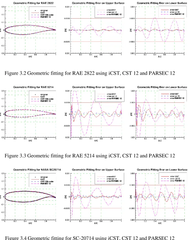
Figure 3.2 Geometric fitting for RAE 2822 using iCST, CST 12 and PARSEC 12 ... 54
Figure 3.3 Geometric fitting for RAE 5214 using iCST, CST 12 and PARSEC 12 ... 54
Figure 3.4 Geometric fitting for SC-20714 using iCST, CST 12 and PARSEC 12 ... 54
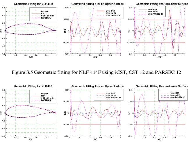
Figure 3.5 Geometric fitting for NLF 414F using iCST, CST 12 and PARSEC 12 ... 55
Figure 3.6 Geometric fitting for NLF 416 using iCST, CST 12 and PARSEC 12 ... 55
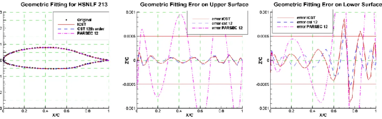
Figure 3.7 Geometric fitting for HSNLF 213 using iCST, CST 12 and PARSEC 12 ... 56
Figure 3.8 Geometric fitting for S805A using iCST, CST 12 and PARSEC 12 ... 56
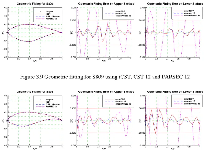
Figure 3.9 Geometric fitting for S809 using iCST, CST 12 and PARSEC 12 ... 57
Figure 3.10 Geometric fitting for S825 using iCST, CST 12 and PARSEC 12 ... 57
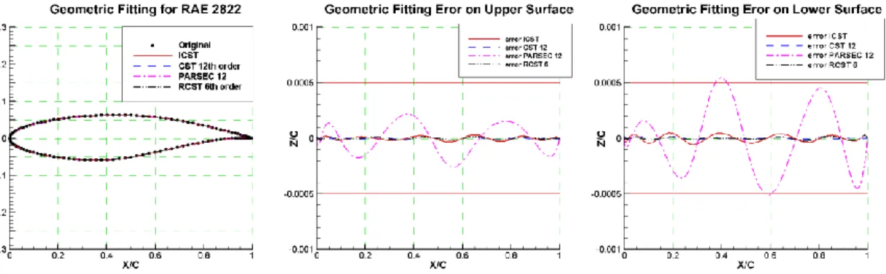
Figure 3.11 Geometric fitting for RAE 2822 using 6th order RCST... 60
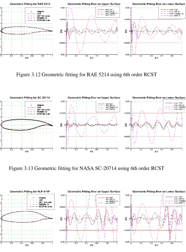
Figure 3.12 Geometric fitting for RAE 5214 using 6th order RCST... 61
Figure 3.13 Geometric fitting for NASA SC-20714 using 6th order RCST ... 61
Figure 3.14 Geometric fitting for NLF 414F using 6th order RCST ... 61
Figure 3.15 Geometric fitting for NLF 416 using 6th order RCST ... 62
Figure 3.16 Geometric fitting for HSNLF 213 using 6th order RCST ... 62
Figure 3.17 Geometric fitting for S805A using 6th order RCST ... 62
Figure 3.18 Geometric fitting for S809 using 6th order RCST ... 63
Figure 3.19 Geometric fitting for S825 using 6th order RCST ... 63
Figure 4.1 Wing aerofoil section definition in the CST method ... 67
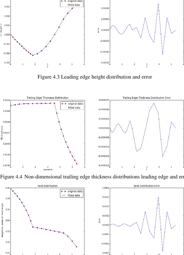
Figure 4.2 Leading edge x coordinates distribution and error ... 71
ix Figure 4.4 Non-dimensional trailing edge thickness distributions leading edge and error
... 72
Figure 4.5 Tangential value of twist angle distributions and error ... 72
Figure 4.6 Local chord distributions and error ... 73
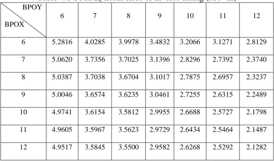
Figure 4.7 The error contour of wing inverse fitting with BPOX 6-BPOY 6 (left figure in metre) and BPOX 6-BPOY 10 (right figure in metre) ... 74
Figure 4.8 The error contour of wing inverse fitting with BPOX 6-BPOY 12 (left figure in metre) and BPOX 10-BPOY 6 (right figure in metre) ... 75
Figure 4.9 The error contour of wing inverse fitting with BPOX 10-BPOY 10 (left figure in metre) and BPOX 12-BPOY 6 (right figure in metre) ... 75
Figure 4.10 The error contour of wing inverse fitting with BPOX 12-BPOY 10 (left figure in metre) and BPOX 12-BPOY 12 (right figure in metre) ... 75
Figure 4.11 The hybrid mesh of F6 wing for CFD study ... 77
Figure 4.12 The sections index and position on the wing... 78
Figure 4.13 Comparisons of pressure distribution and wing shape on section 1 ... 79
Figure 4.14 Comparisons of pressure distribution and wing shape on section 2 ... 80
Figure 4.15 Comparisons of pressure distribution and wing shape on section 3 ... 80
Figure 4.16 Comparisons of pressure distribution and wing shape on section 4 ... 81
Figure 4.17 Comparisons of pressure distribution and wing shape on section 5 ... 82
Figure 4.18 Comparisons of pressure distribution and wing shape on section 6 ... 83
Figure 4.19 Comparisons of pressure distribution and wing shape on section 7 ... 83
Figure 4.20 Comparisons of pressure distribution and wing shape on section 8 ... 84
Figure 4.21 The HTP model using the CST methods ... 85
Figure 4.22 The VTP model using the CST methods ... 86
Figure 4.23 The error contour of wing inverse fitting with RCST BPOX 6-BPOY 6 (in metre) ... 87
Figure 4.24 Comparisons of pressure distribution and wing shape at 10% span ... 89
Figure 4.25 Comparisons of pressure distribution and wing shape at 20% span ... 89
Figure 4.26 Comparisons of pressure distribution and wing shape at 30% span ... 90
Figure 4.27 Comparisons of pressure distribution and wing shape at 40% span ... 90
x
Figure 4.29 Comparisons of pressure distribution and wing shape at 60% span ... 91
Figure 4.30 Comparisons of pressure distribution and wing shape at 70% span ... 91
Figure 4.31 Comparisons of pressure distribution and wing shape at 80% span ... 91
Figure 4.32 Comparisons of pressure distribution and wing shape at 90% span ... 92
Figure 4.33 The wing with winglet-1: wing in blue, transition part in green, winglet in red ... 96
Figure 4.34 The leading edge lines control points ... 97
Figure 4.35 The leading edge lines of transition part and winglet on the y-z plane ... 98
Figure 4.36 The extension of the wing on the y-z plane ... 99
Figure 4.37 The planform parameters for wing extension on the x-y plane ... 100
Figure 4.38 The leading and trailing edge lines and control point and polygon for wing extension on the x-y plane ... 101
Figure 4.39 The surface of wing extension ... 104
Figure 4.40 The translation relationship between wing extension and winglet-1 ... 105
Figure 4.41 The rotation relationship... 106
Figure 4.42 The translation view on the x-y plane ... 106
Figure 4.43 The winglet-2 leading edge on the y-z plane and planform parameters... 108
Figure 4.44 The planform parameters of wing extension for winglet-2 on the x-y plane ... 108
Figure 4.45 The surface of wing extension for winglet-2 on the x-y plane ... 109
Figure 4.46 The translation of wing extension to winglet-2 ... 109
Figure 4.47 The surface of winglet-2 ... 110
Figure 4.48 The winglet-3... 111
Figure 4.49 The winglet-4... 111
Figure 4.50 The three main parts of the fuselage... 112
Figure 4.51 The CST parametric mid-part fuselage component... 112
Figure 4.52 The forward part fuselage of an F4 aircraft with cabin ... 114
Figure 4.53 The CST parametric forward part fuselage ... 115
Figure 4.54 A CAD tail cone model ... 116
Figure 4.55 The CST parametric tail cone ... 117
xi
Figure 4.57 The CST belly-fairing parametric model ... 121
Figure 4.58 The error contour of belly-fairing inverse fitting with BPOX 6-BPOY 6 (left figure) and BPOX 8-BPOY 8 (right figure) ... 122
Figure 4.59 The error contour of belly-fairing inverse fitting with BPOX 10-BPOY 10 (left figure) and BPOX 12-BPOY 12 (right figure) ... 122
Figure 4.60 The nacelle inlet using PARSEC intuitive parameters ... 124
Figure 4.61 The CST parametric nacelle model ... 125
Figure 4.62 The CST parametric model of FTF ... 127
Figure 4.63 A pylon CAD model ... 128
Figure 4.64 A simplified pylon model without root fairing... 129
Figure 4.65 CST parametric model of a simplified pylon ... 130
Figure 4.66 Parameterisation for 2D shock control bump using piecewise polynomials (Wong 2006) ... 132
Figure 4.67 The bump curve using the CST methods ... 133
Figure 4.68 The 1st derivative distribution of bump curve using the CST method ... 134
Figure 4.69 The 2nd derivative distribution of bump curve using the CST method... 134
Figure 4.70 The intersection lines of two high free-form surfaces ... 138
Figure 4.71 The intersection line between wing and belly-fairing ... 139
Figure 4.72 The approximation of step length ... 142
Figure 4.73 The important points on intersection line (Huang and Zhu 1997) ... 144
Figure 4.74 The example of intersection line between fuselage and belly-fairing ... 146
Figure 5.1 The control volume i in the finite volume method ... 155
Figure 5.2 The flux between cells i and j ... 156
Figure 5.3 The cell-vertex finite volume: black nodal points and grey lines form the primary grid, black lines form the secondary grid ... 157
Figure 5.4 Surrounding points used for the least square algorithm ... 161
Figure 6.1 The vector of over the surface of RAE 2822 aerofoil for drag ... 179
Figure 6.2 The vector of over the surface of RAE 2822 aerofoil for lift ... 179
Figure 6.3 The pressure distribution of RAE 2822 ... 180
Figure 6.4 Validation of gradient of Cd for RAE 2822 using CST 7th order ... 181
xii Figure 6.6 Blending function for grid node deformation computation, including the
parameter radius full weight (RFW) and radius zero weight (RZW) ... 194
Figure 6.7 Adjoint optimisation framework of Surfgard ... 196
Figure 7.1 Mesh of RAE 2822 ... 200
Figure 7.2 Cd (left) and Cl (right) optimisation history of 7th order CST ... 201
Figure 7.3 Cd (left) and Cl (right) optimisation history of 10th order CST ... 201
Figure 7.4 The contour of pressure coefficients of initial aerofoil (left) and optimum aerofoil (right) obtained by 7th order CST ... 202
Figure 7.5 The contour of pressure coefficients of initial aerofoil (left) and optimum aerofoil (right) obtained by 10th order CST ... 203
Figure 7.6 Cp distributions of initial aerofoil and optimal aerofoil obtained by 7th order CST and 10th order CST ... 203
Figure 7.7 Cd (left) and Cl (right) optimisation history of iCST ... 204
Figure 7.8 The contour of pressure coefficients of initial aerofoil (left) and optimum aerofoil (right) obtained by iCST ... 205
Figure 7.9 Cp distributions of initial and optimal aerofoils obtained by iCST method .. 206
Figure 7.10 Cd (left) and Cl (right) optimisation history of RCST ... 207
Figure 7.11 The contour of pressure coefficients of initial aerofoil (left) and optimum aerofoil (right) obtained by RCST ... 208
Figure 7.12 Cp distributions of initial and optimal aerofoils obtained by RCST method ... 208
Figure 7.13 Comparison of the initial aerofoil and optimal aerofoils obtained by various parameterisation methods ... 209
Figure 7.14 Optimisation of drag using CST bump ... 212
Figure 7.15 Optimisation of drag using PARSEC bump ... 212
Figure 7.16 Optimisation of drag using standard cubic bump ... 212
Figure 7.17 Contour of pressure coefficient of aerofoil without bump (left) and aerofoil with optimal CST bump (right)... 213
Figure 7.18 Contour of pressure coefficient of aerofoil without bump (left) and aerofoil with optimal PARSEC bump (right) ... 213
xiii Figure 7.19 Contour of pressure coefficient of aerofoil without bump (left) and aerofoil
with optimal standard cubic bump (right) ... 214
Figure 7.20 Comparison of Cp distribution ... 214
Figure 7.21 Comparison of bump shape ... 215
Figure 8.1 Optimisation history of drag (left) and the 10th torsion box volume (right) using CST with BPOX 6-BPOY 6 ... 221
Figure 8.2 Optimisation history of drag (left) and the 10th torsion box volume (right) using CST with BPOX 6-BPOY 8 ... 221
Figure 8.3 Optimisation history of drag (left) and the 10th torsion box volume (right) using CST with BPOX 6-BPOY 10 ... 222
Figure 8.4 Optimisation history of drag (left) and the 10th torsion box volume (right) using CST with BPOX 10-BPOY 10 ... 222
Figure 8.5 The Cp contour plot of initial wing surface, lower (left) and upper (right) .. 223
Figure 8.6 The Cp contour plot of optimal wing surface, lower (left) and upper (right), obtained by CST with BPOX 6 and BPOY 6 ... 223
Figure 8.7 The Cp contour plot of optimal wing surface, lower (left) and upper (right), obtained by CST with BPOX 6 and BPOY 8 ... 224
Figure 8.8 The Cp contour plot of optimal wing surface, lower (left) and upper (right), obtained by CST with BPOX 6 and BPOY 10 ... 224
Figure 8.9 The Cp contour plot of optimal wing surface, lower (left) and upper (right), obtained by CST with BPOX 10 and BPOY 10 ... 225
Figure 8.10 Cp distribution (left) and aerofoil shapes (right) at 10% span of wing ... 226
Figure 8.11 Cp distribution (left) and aerofoil shapes (right) at 30% span of wing ... 226
Figure 8.12 Cp distribution (left) and aerofoil shapes (right) at 50% span of wing ... 226
Figure 8.13 Cp distribution (left) and aerofoil shapes (right) at 70% span of wing ... 227
Figure 8.14 Cp distribution (left) and aerofoil shapes (right) at 80% span of wing ... 227
Figure 8.15 Cp distribution (left) and aerofoil shapes (right) at 90% span of wing ... 227
Figure 8.16 Twist distribution ... 230
Figure 8.17 The spanwise lift distribution ... 231
Figure 8.18 Optimisation history of drag (left) and Cmx (right) using CST with BPOX 6-BPOY 6... 233
xiv Figure 8.19 Optimisation history of the 10th torsion box volume using CST with BPOX 6-
BPOY 6... 233
Figure 8.20 The Cp contour plot of optimal wing surface, lower (left) and upper (right), obtained by CST with BPOX 6 and BPOY 6 in optimisation with Cmx constraint ... 234
Figure 8.21 Cp distribution (left) and aerofoil shapes (right) at 10% of wingspan ... 234
Figure 8.22 Cp distribution (left) and aerofoil shapes (right) at 30% of wingspan ... 235
Figure 8.23Cp distribution (left) and aerofoil shapes (right) at 50% of wingspan ... 235
Figure 8.24 Cp distribution (left) and aerofoil shapes (right) at 70% of wingspan ... 236
Figure 8.25 Cp distribution (left) and aerofoil shapes (right) at 80% of wingspan ... 236
Figure 8.26 Cp distribution (left) and aerofoil shapes (right) at 90% of wingspan ... 236
Figure 8.27 Twist distribution ... 237
Figure 8.28 The lift distribution along span... 238
Figure 8.29 Optimisation history of drag (left) and Cmx (right) using RCST with BPOX 6 -BPOY 6 ... 240
Figure 8.30 Optimisation history of the 10th torsion box volume using RCST with BPOX 6- BPOY 6 ... 240
Figure 8.31 The Cp contour plot of Initial wing surface, lower (left) and upper (right), which is represented by RCST with BPOX 6 and BPOY 6... 241
Figure 8.32 The Cp contour plot of optimal wing surface, lower (left) and upper (right), obtained by RCST with BPOX 6 and BPOY 6 in optimisation with Cmx constraint ... 241
Figure 8.33 Cp distribution (left) and aerofoil shapes (right) at 10% of wingspan ... 242
Figure 8.34 Cp distribution (left) and aerofoil shapes (right) at 30% of wingspan ... 242
Figure 8.35Cp distribution (left) and aerofoil shapes (right) at 50% of wingspan ... 243
Figure 8.36 Cp distribution (left) and aerofoil shapes (right) at 70% of wingspan ... 243
Figure 8.37 Cp distribution (left) and aerofoil shapes (right) at 80% of wingspan ... 243
Figure 8.38 Cp distribution (left) and aerofoil shapes (right) at 90% of wingspan ... 244
Figure 8.39 Twist distribution ... 245
Figure 8.40 The lift distribution along span... 245
Figure 8.41 Optimisation history of drag of winglet-1 (left) and winglet-2 (right) ... 252
xv Figure 8.43 The Cp contour and zoomed in view with Cf lines of initial design of
winglet-1 ... 254
Figure 8.44 The Cp contour and zoomed in view with Cf lines of optimised design of winglet-1 ... 255
Figure 8.45 The Cp contour and zoomed in view with Cf lines of initial design of winglet-2 ... 255
Figure 8.46 The Cp contour and zoomed in view with Cf lines of optimised design of winglet-2 ... 256
Figure 8.47 Cl (left) and Cd wave drag (right) distribution along span of winglet-1 ... 256
Figure 8.48 Cl (left) and Cd wave drag (right) distribution along span of winglet-2 ... 257
Figure 8.49 Cp Contour of initial and optimised winglet-3 ... 259
Figure 8.50 Cp Contour of initial and optimised winglet-4 ... 260
Figure 8.51 Cl (left) and Cd wave drag (right) distribution along span of winglet-3 ... 260
Figure 8.52 Cl (left) and Cd wave drag (right) distribution along span of winglet-4 ... 261
Figure 8.53 Cd pressure drag (left) and friction drag (right) of optimal results of four types of winglet ... 261
Figure 8.54 Sensitivities of Cd to surface point Z direction and boundaries of bumps .. 263
Figure 8.55 Optimisation history of Cd ... 264
Figure 8.56 Optimised 12 bumps on wing ... 265
Figure 8.57 Surface Cp contour in range -1.2 to -0.4 of initial wing without bump(left) and optimised bumps (right) ... 265
Figure 8.58 Cp Contour and Cf lines plot on upper surface of initial wing without bump (left) and optimised bumps (right) ... 266
Figure 8.59 Cp distribution and aerofoil section cut at middle of bump 1 ... 266
Figure 8.60 Cp distribution and aerofoil section cut at middle of bump 5 ... 267
Figure 8.61 Cp distribution and aerofoil section cut at middle of bump 9 ... 267
Figure 8.62 Cp distribution and aerofoil section cut at middle of bump 12 ... 267
xvii
List of Tables
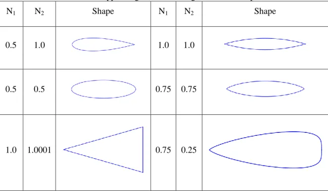
Table 2.1 Various types of geometries using different class parameters ... 36
Table 4.1 Total L2 norm error of inverse fitting (x10-2m) ... 74
Table 4.2 Lift coefficient of original geometry and approximated geometry ... 77
Table 4.3 Drag coefficient of original geometry and approximated geometry ... 77
Table 4.4 Lift coefficient of original geometry and RCST approximated geometry ... 88
Table 6.1 Common radial basis function ... 189
Table 7.1 Aerodynamic coefficients and constraint values ... 202
Table 7.2 Aerodynamic coefficients and constraint values ... 205
Table 7.3 Aerodynamic coefficients and constraint values ... 207
Table 7.4 Aerodynamic coefficients ... 215
Table 8.1 Torsion box volume of initial geometry ... 220
Table 8.2 Aerodynamic coefficients (drag units in drag count) ... 229
Table 8.3 Aerodynamic coefficients of optimal results (drag units in drag count) ... 238
Table 8.4 Aerodynamic coefficients of optimal results using RCST (drag units in drag count) ... 246
Table 8.5 Planform parameters of winglet-1 ... 248
Table 8.6 Planform parameters of winglet-2 ... 249
Table 8.7 Planform parameters of winglet-3 ... 250
Table 8.8 Planform parameters of winglet-4 ... 251
Table 8.9 Aerodynamic coefficients of winglet-1 (drag unit in drag count) ... 253
Table 8.10 Aerodynamic coefficients of winglet-2 (drag unit in drag count) ... 253
Table 8.11 Aerodynamic coefficients of winglet-3 (drag unit in drag count) ... 258
Table 8.12 Aerodynamic coefficients of winglet-4 (drag unit in drag count) ... 258
xviii
Nomenclature
Roman Symbols
Ai = Weighting coefficient of shape function
Aup,lo, Bup,lo = Matrices and vectors of design parameters for upper and lower surfaces ai,bi = Coefficients of PARSEC polynomials
b = Wing span
Bui,j, Bli,j = Upper and lower wing surface weight factors BPO = Order of the Bernstein polynomial
BPOX = Order of the Bernstein polynomial for chordwise
BPOY = Order of the Bernstein polynomial for spanwise
c = Chord length
CLocal = Local chord length
CFD = Computational Fluid Dynamics
CST = Class/Shape function transformation
= Class function Cd = Drag coefficient Cl = Lift coefficient
Cmx = Rolling momentum coefficient Cp = Pressure coefficient
C1,C2 = First and second surface derivatives = The i-th inequality constraint function
= The j-th equality constraint function
D = Design variables
= The artificial dissipation term
E = Total energy per control volume f = Body force in linear elasticity
= Convective flux
xix FFD = Free-form deformation
FTF = Flap track fairing HTP = Horizontal tail plane
H = Total enthalpy = Height of fuselage
= Local crown height of fuselage nose profile (relate with crown line)
iCST = Intuitive CST
I = Cost function
= Local keel height of fuselage nose and tail cone profile (relate with Keel line)
Kr,n = Binomial coefficient
K = Stiffness matrix of the mesh deformation system
= Spring stiffness model between two adjacent grid nodes
k = kinetic energy
L2 = L2-norm
= Bump length at beginning of boundary side MDO = Multi-disciplinary optimisation
n = Order of Bernstein polynomials
N1,N2,Nc =Class function exponents
NDV = Number of design variables
Nx = Order of Bernstein Polynomial in chordwise Ny = Order of Bernstein Polynomial in spanwise NURBS = Non-uniform Rational B-Spline
PARSEC = Parametric aerofoil section
= Control points vector of Bezier Curve, control points of winglet plant form
= Pressure
q = Heat flux
R = Radius on cylindrical coordinate, Flow residual in flow and adjoint equation
xx
Rcrown,Rkeel = Radius on cylindrical coordinate when 1.5and Rle,upper Rle,lower = Leading edge radius on upper lobe and lower lobe of nacelle Rle = Leading edge radius
s = Approximated function in Radial Basis Function mesh deformation = Search direction in the design space
= Shape function
= Rational Shape function
, = Bernstein polynomials in span and chordwise
T = Temperature, the residual vector of mesh deformation in the mesh adjoint approach
= Time
TEnd, up TEnd, lo = Tangential value of upper and lower ends of inlet
= Total length of component
= Non-dimensional coordinate in Bezier Curve, velocity component in x direction
v = Velocity component in y direction
VTP = Vertical tail plane = Volume of cell k
W = Conservative state vector
w = Velocity component in z direction
Wi = Weights coefficients in rational equation
Fuselage
W = Width of fuselage
= Local width of fuselage nose and tail cone profile, (relate with side line) Winglet-1 = Upward winglet with a transition part and straight winglet part
Winglet-2 = Upward winglet only with a smooth winglet part
Winglet-3 = Downward winglet with a transition part and straight winglet part Winglet-4 = Downward winglet only with a smooth winglet part
X = Grid variable
= Surface mesh points = Volume mesh points
xxi
XLE = Leading edge position in x coordinate in wing CST representation XLO =Lower throat x position of nacelle inlet
XUP = Upper throat x position of nacelle inlet XEnd, up, = Upper end station of nacelle inlet XEnd, lo, =Lower end station of nacelle inlet ZEnd, up = Upper end z position of nacelle inlet ZEnd, lo = Lower end z position of nacelle inlet
ZLO = Lower throat height of nacelle inlet, z coordinate on aerofoil lower
surface
ZUP = Upper throat height of nacelle inlet, z coordinate on aerofoil lower
surface
Xup = X coordinates of aerofoil crest on upper surface Xlo = X coordinates of aerofoil crest on lower surface
X1,upX2,up = X coordinates of two iCST design points on upper surface X3,lo X4,lo = X coordinates of two iCST design points on lower surface Vup,lo = Vectors of coefficients of polynomials
Zup = Z coordinates of crest on upper surface Zlo = Z coordinates of crest on lower surface
Zxx,up = Second derivative at crest on upper surface, (at throat in nacelle) Zxx,lo = Second derivative at crest on lower surface, (at throat in nacelle) Zte = Z coordinate of aerofoil trailing mid-point
Z1,up Z2,up = Z coordinates of two iCST design points on upper surface Z3,lo Z4,lo = Z coordinates of two iCST design points on lower surface Zx,1,up Zx,2,up = First derivative at two iCST design points on upper surface Zx,3,lo Zx,4,lo = First derivative at two iCST design points on lower surface Zxx,1,up Zxx,2,up = Second derivative at two iCST design points on upper surface Zxx,3,lo Zxx,4,lo = Second derivative at two iCST design points on lower surface
Centre
Z = Coordinate of local profile centre of fuselage nose and tail cone
xxii Greek Symbols
αtwist = Local wing twist angle
α = Angle of attack
= Coefficient of Radial Basis Function mesh deformation = Sweep angle of leading edge of transition part of winglet 1 = Sweep angle of trailing edge of transition part of winglet 1 = Sweep angle of leading edge of winglet part of winglet 1 = Sweep angle of trailing edge of winglet part of winglet 1 = Winglet tip dihedral angle of winglet 1
= Leading edge sweep angle of bump = Trailing edge sweep angle of bump
= Sweep angle of leading edge at winglet tip of winglet 2 = Sweep angle of trailing edge at winglet tip of winglet 2
αte = Trailing edge angle
βte = Trailing edge wedge angle
= Coefficient of Radial Basis Function mesh deformation
θup,lo = Trailing edge angle of upper or lower surface ψ = Non-dimensional coordinate in chordwise
= Non-dimensional spacewise coordinate = Local laminar bulk viscosity
= Thermal conductivity
= Adjoint operator for flow equation = Adjoint operator for mesh deformation
= Flow density
= Rotation angle of winglet section along z-axis = Rotation angle of winglet section along x-axis
= Non-dimensional angle on cylindrical coordinate
= Angle on cylindrical coordinate, trailing edge tangential angle = Hicks-Henne function design variables
xxiii γ = Constant specific heat
= Non-dimensional local aerofoil installation height
= Non-dimensional coordinate in direction normal to chordwise
= Trailing edge thickness ratio in CST = Non-dimensional upper surface coordinate = Non-dimensional lower surface coordinate = Non-dimensional trailing edge thickness
= Shear stress
= Stress tensor in linear elasticity = Radial basis function
= Volume of control element
= Non-dimensional chordwise coordinate (in aerofoil or wing), non-dimensional coordinate along body axis (in non-wing type components)
1
Chapter 1
Introduction
1.1Background
Computational aerodynamics has been employed to assist aircraft design for more than six decades. With the development of high performance computers, computational aerodynamic flow solutions have become much less expensive than large-scale experiments for the right Reynolds and Mach numbers. Therefore, computational aerodynamics has been widely employed in the aircraft industry, and is playing an increasingly important role in aircraft design.
Computational aerodynamics tools have developed from the simple low-fidelity panel method to the more complex high-fidelity Reynolds averaged Navier-Stokes (RANS) solution methods. Nowadays, the low-fidelity methods are able to provide results in a very short time and are used for the concept design process; they are effective for assisting the designer in the analysis of technical and economic feasibility for future projects. The high-fidelity methods, such as the Euler equation, RANS and large eddy simulation (LES), are able to provide more accurate results and are normally used in the preliminary and detail design stages.
The pursuit of excellent design is invariably the goal for aircraft designers. Based on Figure 1.1, it has been estimated that the fuel efficiency of a current civil jet transport aircraft, e.g. Airbus A330-300, has been reduced by 70% from the Comet 4 of the 1950s, with 30% coming from advanced airframe design and 40% due to improvement of aero-engines (Mann and Elsholz 2005). The Strategic Research Agenda (ACARE 2002; Mann and Elsholz 2005), prepared by ACARE (Advisory Council for Aeronautical Research in Europe), set the direction for European research to reduce the environmental impact of aircraft and to improve safety and operational efficiency. ‘Vision2020’ requires a step change in aircraft performance, such as 50% CO2 emission reduction and perceived noise reduction (ACARE 2002). This is a huge challenge to aircraft designers, since modern aircraft comprise a large number of highly complicated systems. The traditional manual
2 approach would find it very hard, if not impossible, to satisfy future design requirements. Hence, numerical optimisation techniques based on computational flow solutions have become a critical tool for the aircraft industry to help designers to meet future design challenges.
Figure 1.1 Transport aircraft fuel efficiency (from Penner 1999)
Optimisation is a well-established topic, and its essence is to find the maximum or minimum value of the objective function, which mathematically represents the relationship between the input variables and the objective values. Aerodynamic optimisation requires an automatic design process which is able to take geometric parameters to modify the geometry, to run numerical methods to obtain an objective value and to search for the best design shape. Rapid aerodynamic solution methods such as the penal methods and the lifting surface methods are normally employed for conceptual design and multi-disciplinary optimisation (MDO). The high-fidelity CFD methods are used for the detailed design stage; however, they can result in unaffordable computational cost when applied to aerodynamic optimisation. Therefore, although fidelity aerodynamic optimisation was proposed at almost the same time as CFD, high-fidelity aerodynamic optimisation has developed slowly along with the increase in the performance of digital computers. Jameson (1988) successfully applied a method, called
3 the ‘adjoint’ method, to aerodynamic optimisation. With this method, the computational cost was dramatically decreased and this considerably improved the feasibility of high-fidelity aerodynamic optimisation for the aircraft industry. At present, aerodynamic optimisation is widely employed as an automated tool, from the two-dimensional aerofoil to complex three-dimensional configurations (Anderson 1997; Jameson 2004).
For aerodynamic optimisation, the objective values are normally the aerodynamic performance parameters obtained from the numerical methods, such as lift and drag coefficients, pressure distribution, pitching/bending momentum and others. The input variables are also called design variables and normally represent the geometry using various parameterisation methods. Consequently, the parameterisation methods used have a profound effect on the design space, determining the complexity of the design space and the optimum geometries obtainable. Therefore, the shape parameterisation method is a key technique for the designer in the numerical optimisation process.
The two main objectives of this thesis are to find and develop a parameterisation method for the entire modern civil transport aircraft and to apply it to high-fidelity aerodynamic optimisation using the adjoint approach.
The first task is to develop a geometric parameterisation method for the entire modern civil transport aircraft. There are already many geometric parameterisation methods implemented in aerodynamic optimisation. However, most parameterisation methods can only be applied to individual aircraft components rather than the entire aircraft. A few methods, such as computer-aided-design (CAD) and free form deformation (FFD) parameterisation, can potentially be used to parameterise the entire aircraft. However, these are either too complicated to build into the optimisation framework or they struggle to satisfy some designers’ preferred requirements, such as intuitiveness and generality. Therefore, the author of this thesis has further developed a parameterisation method for the entire civil transport aircraft based on Kulfan’s Class/Shape function transformation methods (CST). This method is able to represent most aircraft aerodynamic components in a universal and efficient way.
4 The second task is to build an aerodynamic optimisation framework and apply this parameterisation method in an adjoint-based optimisation for industrial application. Both two-dimensional aerofoil section and three-dimensional geometry optimisation are conducted in the thesis. The performance of this geometric parameterisation will be examined in the aerodynamic optimisation investigation.
1.2 Outline of thesis
This thesis is split into two parts based on the two main tasks, the first focusing on geometric parameterisation and the second on aerodynamic optimisation using the adjoint approach.
In Part I, current geometric parameterisation methods are reviewed and investigated in Chapter 2. This presents the ideal properties of a parameterisation method which is good for aerodynamic design and optimisation, and gives a review of the most common geometric parameterisation methods employed in aerodynamic optimisation and design. This will also explain why the CST method has been selected for this study.
The following chapters, Chapters 3 and 4, present two new geometric parameterisation methods, iCST method and RCST methods, for two-dimensional aerofoils and the development of the CST methods for the entire aircraft. The PARSEC method, CST method, iCST which is able to parameterise aerofoil with full intuitiveness, and RCST which employs the Rational Bernstein polynomials to improve the accuracy of standard CST methods are presented, and their performance according to accuracy in representing existing aerofoils is also discussed in Chapter 3. The CST method is then extended to parameterise three-dimensional civil transport aircraft components, including wing, horizontal tail plane (HTP), vertical tail plane (VTP), winglet, fuselage, belly-fairing, flap tracking fairing (FTF), pylon and nacelle. The parameterisation methods for each component are discussed in detail in Chapter 4. The performance of CST and RCST methods for 3D wing are investigated in Chapter 4. The CST method for shock control
5 bump is then presented. At the end of Chapter 4, the intersection line calculation method is presented for future entire aircraft optimisation.
In Part II, Chapter 5 presents the flow governing equation and the numerical solver for high-fidelity CFD optimisation based on the RANS equations. The optimisation method is presented in Chapter 6 with a literature review of related aerodynamic optimisation methods, the discrete adjoint methodology, the mesh deformation strategy and the optimisation framework. The review focuses on current optimisation techniques applied in aerodynamic optimisation. Chapter 7 shows the two-dimensional optimisation test and results, and includes aerofoil optimisation and aerofoil with bump optimisation for transonic conditions. It examines the performance of the CST parameterisation methods in optimisation, leading to the later three-dimensional optimisation. Chapter 8 shows the three-dimensional optimisation results, including optimisation for the F6 wing, the F6 wing with different types of winglets and shock control bumps on 3D wing optimsiation. Finally, Chapter 9 gives the conclusion of this thesis and provides some suggestions for future work.
6
Chapter 2
Literature Review of Geometric
Parameterisation
This chapter presents the various typical geometric parameterisation methods and their application in aerodynamic optimisation by previous researchers. This gives a background of current state-of-the-art geometric parameterisation methods and an understanding of the basic methodology of parameterisation. The advantages and disadvantages of the various methods will also be discussed.
‘Parameterisation’ is the representation of the specifications of a model as a set of parameters. In aerodynamic optimisation, parameterisation is usually applied to the representation of geometry. These geometric parameters are then employed as design variables for the designer or as input of an optimisation to find a desirable geometry which satisfies required performance.
Samareh (2001) and Kulfan (2006) have pointed out that a well-behaved parameterisation method should have the following properties:
1) To provide high flexibility to cover the potential optimal solution in the design space,
2) To give as small number of design variables as possible, 3) To produce smoothness and realisability of the shapes,
4) To provides intuitiveness of the design parameters for geometrical and physical understanding by the design engineers in exploring the design space and setting up optimisation constraints,
5) To provides grid sensitivity derivatives of grid respect to design variable, which is important for gradient-based optimisation.
In actual applications, a balance needs to be struck for parameterisation, as it is unlikely that all the requirements can be satisfied. For example, parameterisation methods with a
7 high number of design variables are normally able to provide a highly flexible design space; however, the high number of design variables will increase the complexity of the design space and will require that the optimiser makes an extra effort to find the optimum solution. In general, the cost of optimisation based on high-fidelity CFD computation is still very high; it will cause unaffordable computational expense. Even if the adjoint method is applied to be numerically efficient in calculating the sensitivities in gradient-based optimisation (Jameson 1988; Jameson et al. 1997; Le Moigne and Qin 2004; 2006), finding global optimum from a highly complex design space is still a challenging issue. On the other hand, for example, the NACA 4-series aerofoil definition only uses three parameters (maximum camber, position of maximum camber and maximum thickness) to represent an aerofoil (Ladson et al 1996), which are unable to provide sufficient design space to satisfy the desired aerodynamic performance.
Samareh (2001) reviewed and compared some of these methods and classified the shape parameterisation methods into the following eight categories: the basis vector, domain element, partial differential equation, discrete (mesh point), polynomial and spline, analytical, CAD-based and free-form deformation (FFD) methods. Among these methods, the discrete, analytical, polynomial, spline, CAD and FFD are the most common. They are studied and reviewed in the following sections. Another two methods, the parametric aerofoil section method (PARSEC) and the class/shape function transformation method (CST), are presented at the end.
2.1 Discrete methods
The discrete approach, which is the simplest way to do parameterisation, uses the mesh points as design variables. The discrete methods are able to provide a large design space since there is not any natural limit of design space, and theoretically it is possible to represent any shape. It is also easy to set up for any kind of geometry. Therefore, many researchers have tried to use discrete methods in aerodynamic optimisation (Jameson 1988; Campbell 1992; Jameson et al. 1997; Mousavi et al. 2007; Wu et al. 2003; Castonguay and Nadarajah 2007).
8 However, there are two main drawbacks of discrete methods. The first is that it is hard to maintain smoothness of geometry since each surface point is moved individually. Therefore, a smoothing algorithm is required to maintain the smoothness if the geometry. Moreover, in gradient-based optimisation, the gradients along grid points are normally not smooth. As a consequence, a smoothing algorithm will also be required to obtain a smooth gradient (Jameson 1988).
The most important drawback of the discrete method is that it results in a large number of design variables. As stated at the beginning, this will generate a very high dimensional design space. As a result, the complexity of the design space could reduce the efficiency of the optimiser in searching for global optimum and lead to unaffordable computational cost in the aerodynamic optimisation, although local optimum can be obtained efficiently with the adjoint method. Additionally, another drawback of discrete methods is difficult to provide intuitive parameters, for example, sweep angle, thickness, twist and so on. 2.2 Analytical methods
As presented above, although the discrete method is able to provide the most flexible design space, it is not good for reducing the complexity of design space as a large number of design variables are used. A parameterisation method with a small number of design variables that produces a smooth shape is preferred for aerodynamic optimisation. The most efficient way is to put a set of mathematical functions on the geometry surface, which is defined as Equation 2.1:
2.1 where is used as design variable, n is the number of design variables and is the shape function.
The shape functions could be Hicks-Henne functions, Wagner functions, Legendre functions, Bernstein functions or NACA series aerofoil functions. The method is able to support direct representation function without adding any initial geometry.
9 The most common analytical method is called the ‘Hicks-Henne’ shape function method. It was first introduced by Hicks and Henne in 1978. It employs a set of bump basis shape functions, as defined in Equation 2.2:
where
2.2
defines the position of maximum peak point of the i-th bump function, and w controls the width of the bump function.
Khurana et al. (2008) conducted a study of analytical parameterisation methods by comparing five different shape functions, including the Hicks-Henne, Wagner, Legendre, Bernstein, and NACA normal modes. In order to examine their impact on design space. The first work was to carry out an aerofoil geometric fitting study using these five functions, with the NACA 0015 aerofoil being used as a baseline shape. The NASA LRN (1)-1007, NASA LS-0417, NASA NLF (1)-1015 aerofoils were employed as target aerofoils. Five shape functions were used to fit three target aerofoils under a Particle Swarm Optimisation (PSO) algorithm and a linear search method. The speed of convergence and accuracy of the approximation were compared and the design variables, from 4 to 20, were examined for each method. The results showed that the optimisation could converge very fast when using four variables. However, the accuracy with four variables was less than that with 20 variables. The results which were obtained using the five functions were compared. The Hicks-Henne function provided the highest fitting accuracy of all the types of function within relative convergence speed. Thus, the Hicks-Henne function was found to be a better aerofoil shape representation method than the others. The performance of the Hicks-Henne shape function in aerodynamic optimisation was also examined in the second part of this work by carrying out an inverse design process. The results demonstrated that the Hicks-Henne function would provide good results when it is applied to an inverse design for an aerofoil at high Reynolds number condition. However, it generated some oscillations on a Cp distribution for the case at a low Reynolds number due to unsmooth shape. Eyi and Lee (1997) employed the Hicks-Henne and Wagner functions as smooth perturbations to the initial geometry in a
two-10 dimensional aerofoil inverse design optimisation. The test showed that both the Hicks-Henne and Wagner methods could achieve the target aerofoil and the convergence speed of the Wagner functions is slightly faster than the Hicks-Henne functions.
The Hicks-Henne method has been widely employed in aerodynamic optimisation studies. Sung and Kwon. (2001) employed 15 Hicks-Henne functions to modify an aerofoil, and used 5 sections with 10 Hicks-Henne functions on each section to modify a wing shape. Kim, Sasaki et al. (2001) carried out a wing-body-nacelle and a wing-body aerodynamic optimisation study with Hicks-Henne functions. The wing is defined as 5 sections with 20 Hicks-Henne functions for each section plus planform height parameters. The total number of design variables is only 106 for this three-dimensional configuration. After optimisation, the shock wave was greatly reduced. Kim et al. (2002) performed an aerodynamic optimisation test for a high-lift device. A two-dimensional multi-element aerofoil was represented by 157 design variables, of which 50 were Hicks-Henne functions for each master element, three rigging variables for the slat and flap element, and one for angle of attack. Nakayama et al. (2006) carried out a similar two-dimensional multi-element aerofoil optimisation. The total number of design variables was decreased to 71, of which 65 were design variables for aerofoil, slat and flap, eight variables for position of slat and flap and two variables for slat and flap angle. Kim and Nakahashi (2005) carried out a high-lift device optimisation with the unstructured adjoint method. A multi-element aerofoil with vane and flap was modified and the Hicks-Henne shape functions were employed to parameterise the geometry. The total number of design variables was 37, with 10 functions for vane upper and lower surfaces and flap leading edge area respectively. More Hicks-Henne applications can be found in Hageri et al.
(1994), Kim and Alonso (2002a, 2002b), Zuo et al. (2006), Reuther et al. (1996; 1999), Elliott and Peraire (1996), Kim et al. (1999), Nadarajah and Jameson (2000), Eyi et al. (1996) and others.
2.3 Polynomial, spline methods, CAD-based and free-form deformation
Other techniques to represent geometry shapes with reduced number of design variables are polynomials and splines. The polynomial method is the basic method to represent
11 curves with an easy mathematical power form function and high computational efficiency. The polynomial curves can be written as:
2.3 where the polynomial of n-th order, R(u), is the value of the polynomial function, Ai are
coefficients of polynomials and normally used as design variables to control curves. It can be in either implicit or explicit form. The low order polynomial form performs well for representing a simple curve. For a complex curve, a high order polynomial is required to provide move flexibility. However, high order polynomials will easily produce oscillations and cause numerical instability issues. In addition, the power form basis polynomial provides less intuitive information to the designer, such as starting and ending point positions and tangential values. Therefore, it is normally employed to parameterise simple curves in aerodynamic components, such as leading edge and twist distribution function (Le Moigne 2002).
For more complex curves, Bezier and B-spline curves are preferred. The Bezier curve was originally used in the design of automotive bodies and has been widely employed in the aerospace industry. A Bezier curve in n-th order for a single segment is described as:
2.4
where n is the order of Bezier curve (thus the total number of control points is n+1), R(u)
is the vector value of the polynomial function, are the control point vectors which are normally used as design variables in optimisation and is the i-th term of an n-th order Bernstein polynomial, which is defined as:
2.5
where is the binominal coefficient defined as:
12 Once the control points are determined, the Bezier curve can be established. The Bezier curve is bounded by a ‘control polygon’ which is formed of all the control points: see Figure 2.1. The first and last lines of the control polygon coincide with the tangential direction of this Bezier curve at starting and ending points. The details can be found in Appendix A (Piegl and Tiller 1997).
Figure 2.1 Bezier curve with control points
The three-dimensional Bezier surface can be defined by a tensor product form, and shown as: 2.7
where m, n is the order of Bezier surface in i and j direction, R(u) is the vector value of the polynomial function, and , are the control point vectors Many researchers have used the Bezier curve in shape optimisation (Cosentino and Holst 1986; Désidéri et al. 2004) and have presented the Bezier curve as efficiently representing an aerofoil-like curve and providing designers with more interactive control. However, for very complex curves, the Bezier curve is less efficient and more control points are required, as more control points will increase the order of the polynomial. Similarly for the power basis form, higher order polynomials will produce oscillations and cause numerical instability issues. Thus, it is inefficient for representing a very complex curve. Furthermore, any coefficient or control point could affect the entire curve and, therefore, it lacks local control. To overcome these shortages, piecewise polynomials are employed. The
‘B-13 spline curve’ is developed based on this and can be considered as a curve which comprises a few Bezier curves. A pth order B-spline curve can be written as:
2.8
where p is the order of the B-spline curve, R(u) is the coordinate of geometry vector, Pi is
the B-spline control points vector and is the B-spline basis function, which is normally obtained by a recurrence formula, from Boor (1972 and 1977) :
2.9 and 2.10
where ui are the breakpoints, so called ‘knot’ in B-spline methods. For a p-th order
B-spline curve with n control points, m=n+p+1 knots are required. A detailed description and background of B-spline is given in Piegl and Tiller (1997).
B-spline is able to provide an excellent overall shape control, and it also can provide a high capability for local shape control, because the control points only affect the curve on local zone [ui , ui+p+1]. Like the Bezier methods, it can also be extended to represent a
three-dimensional surface, defined as
2.11
Therefore, B-splines have been widely employed in curve and surface design and aerodynamic optimisation research. It provides very high flexible design space with a relatively low number of design variables. Furthermore, because the B-spline has excellent performance in interpolating dataset, it could be employed to interpolate
14 through a few key points on a curve or surface to provide intuitive control of curve or surface.
However, there is a shortcoming of the Bezier and B-spline curves: they are essentially still polynomial-based and cannot naturally accurately represent implicit conic shapes, such as circles, ellipses and hyperbolas. Therefore, there is a special modification, namely ‘rational curves’, which is introduced to overcome this issue by employing another polynomial, the so-called weights. In the spline curve, the non-uniform rational B-spline (NURBS) has been developed (Versprille 1975; Tiller 1983; Piegl and Tiller 1997). The NURBS form is written as:
2.12
where, similarly with B-spline, p is the order of NURBS curve, R(u) is the coordinate of the geometry vector, Pi is the NURBS control points vector and Wi are the weights.
is the B-spline basis function that is the same as the above B-spline curve basis function.
The design variables could be selected either from Pi or Wi. Therefore, the NURBS
inherits the benefits of B-spline, and overcomes B-spline’s shortcomings. The NURBS is capable of accurately representing the quadratic primitives; it is also able to represent the three-dimensional surface, and the definition is:
2.13 where 2.14
Because of B-spline, NURBS have very good performance for curve manipulation; most CAD systems have employed them as a key tool to generate curves and surfaces. The CAD system has a powerful capability for handling complex geometry and has been widely used in the design process. Therefore, using commercial CAD software directly in
15 the optimisation design process as parameterisation, in so-called CAD-based methods, is increasingly interesting for industrial designers and researchers. The benefits of CAD-based methods are stated as:
1) The CAD software is powerful for manipulating very complex geometries, which reduces the researchers’ development time for complex geometries,
2) CAD can provide many intuitive parameters, such as camber, thickness, slots, twist, etc. (Samareh 2001),
CAD has become a standard design tool in different areas, including aerodynamic, structure and system design. Thus, CAD software is also able to provide connectors for different purposes. This would be significant for multi-disciplinary optimisation (MDO).
However, it is still a challenge to embed CAD in an optimisation loop; the main difficulties are:
1) For the most part, CAD can provide accurate and smooth geometry, but it is not perfect. Normally, there are some blemishes, such as gaps, unwanted wiggles and free edges, in the CAD surface model. These may be ignorable in solid design, but are not acceptable for update or regenerate CFD (Samareh 2001).
2) In the gradient-based optimisation technique, the sensitivities of surface points with respect to design variable are required. However, this information is not provided in most current CAD tools (Townsend et al. 1998). Hence, gradient-based high-fidelity optimisation is hardly applied in CAD-gradient-based methods. An alternative way is to calculate surface sensitivities by finite difference (He et al. 1998). However, this requires that the surface topology does not change. Another promising method is developed by Armstrong et al. (2009) using design velocity. 3) The surface topology may be changed when the design variable is updated
(Samareh 2001; Fudge and Zingg 2005). This could cause failure when updating surface CFD mesh and calculating surface sensitivities.
16 4) As a practical issue, the number of CAD licences will be a hurdle for parallel
optimisation processes.
Many researchers have used Bezier, B-spline, NURBS and CAD-based methods in aerodynamic optimisation (Lambert 1995; Tang and Désidéri 2002; Li and Krist 2005; Painchaud-Ouellet et al. 2006; Grasso 2012; Nelson et al. 2005; Fudge and Zingg 2005). Samareh (2001) asserted that B-spline and NURBS are best suited for the two-dimensional optimisation case, because the three-two-dimensional complex geometry requires a large number of control points.
Sasaki and Obayashi (2003) used the B-spline and Bezier surface to represent the wing-fuselage configuration with a total number of 131 design variables. Nemec and Zingg (2002) performed a study of a multi-point and multi-objective aerodynamic optimisation for the design of a two-dimensional single-element and multi-element aerofoil. Fifteen control points were employed to represent a simple NACA 0012 aerofoil, and 10 of 15 control points were employed as design variables. The RAE 2882 aerofoil was represented as 25 control points and 19 control points were used as design variables. Later on, Nemec et al. (2004) carried out an aerodynamic optimisation study based on a CAD system. In order to address the issues of CAD parameterisation methods, a non-commercial CAD library, called Cart3D, was employed rather than using commercial CAD software directly. This CAS library employs the B-spline curve and surface to represent two-dimensional and three-dimensional geometries. A gradient-based optimisation method was used, and the gradient was calculated by finite-difference. A two-dimensional aerofoil optimisation and a complex configuration (fuselage, wing and canard) optimisation were tested. They showed B-spline methods have successfully provide optimal solutions on both 2D and 3D cases and also presented an alternative way of implementing CAD-based parameterisation.
Song and Keane (2004) made a comparative study of two parameterisation methods, which are the basis function derived by Robinson and Keane (2001) and B-spline interpolation methods. Three aerofoils, NACA 0406, NACA 0610 and RAE 2822, were chosen as the target aerofoils. Inverse design optimisation was carried out to examine the