Measuring deprivation in Spain

IRISS at

CEPS/INSTEAD

An Integrated Research

Infrastructure in the Socio-Economic

Sciences

MEASURING DEPRIVATION IN SPAIN

by

Jesús Pérez-Mayo

IRISS WORKING PAPER SERIES

No. 2003-09

RESEARCH GRANTS

for individual or collaborative research projects

(grants awarded for periods of 2-12 weeks)

What is IRISS-C/I?

IRISS-C/I is a project funded by the European Commission in its ‘Access to Major Research Infrastructures’ programme. IRISS-C/I funds short visits at CEPS/Instead for researchers willing

to undertake collaborative and/or internationally comparative research in economics and other social sciences.

Who may apply?

We encourage applications from all interested individuals (doing non-proprietary research in a European institution) who want to carry out their research in the fields of expertise of

CEPS/Instead.

What is offered by IRISS-C/I?

Free access to the IRISS-C/I research infrastructure (office, computer, library…); access to the CEPS/Instead archive of micro-data (including e.g. the ECHP); technical and scientific assistance;

free accommodation and a contribution towards travel and subsistence costs. Research areas

Survey and panel data methodology; income and poverty dynamics; gender, ethnic and social inequality; unemployment; segmentation of labour markets; education and training; social protection and redistributive policies; impact of ageing populations; intergenerational relations;

regional development and structural change. Additional information and application form

IRISS-C/I

B.P. 48 L-4501 Differdange (Luxembourg)

IRISS-C/I

An Integrated Research Infrastructure in the

Socio-Economic Sciences at CEPS/Instead,

Luxembourg

Project supported by the European Commission and the

Ministry of Culture, Higher Education and Research

(Luxembourg)

M

EASURING DEPRIVATION IN

S

PAIN1

Jesús Pérez-Mayo

Department of Applied Economy, University of Extremadura, Campus Universitario, 06071 BADAJOZ (SPAIN)

Fax: 34 924 272 509 e-mail address: [email protected]

Abstract

This paper analyses the deprivation in Spain based on ECHP data for 1996. Usually, an indirect approach for measuring deprivation or poverty is used with poverty lines. That is, income is used as a proxy for analysing living conditions. However, some studies have used a direct approach to measure deprivation or poverty (Townsend 1988, Mayer and Jencks 1988, Muffels 1993, Callan et al 1993, Dirven and Fouarge 1995, Layte et al 1999, Whelan et al 2000). The aim of this paper is improving the identification of the poor people.

The central point of the concept of deprivation we use is related to the opportunity to have or do something. Therefore, deprivation means here an inability to get the goods, facilities and opportunities, which are usual in the household environment.

Since all of the variables needed to build the profiles are categorical, we use the latent class model to solve this problem because it is the best model to do it. This model supplies some clusters that are homogeneous within them and heterogeneous between them.

We have analysed a sample of 6268 households. We have chosen households as the unit of analysis because the variables used in this study appears only in the ECHP Public Use household file. These variables are related to financial situation, housing and durable goods. Firstly, we have found deprivation clusters for each part (financial situation, durable goods, housing facilities, accommodation) and, afterwards, we have built a composite typology in order to identify deprived households.

Keywords: poverty, deprivation, latent class models

JEL codes: I32, I31, C13

1

This research was funded by a grant of the European Commission under the Transnational Access to major Research Infrastructures contract hosted by IRISS-C/I at CEPS/INSTEAD at Differdange (Luxembourg) in 2000. ECHP-UDB 2000 has been used in this study

1. Introduction

According to the European Council (1984), cited in EUROSTAT (2000),

“the poor people are those individuals, families or groups whose material, cultural and social resources are so limited that they are excluded from the minimum standard of living of the society where they live".

In the previous citation, a multidimensional concept of poverty is defined more related to the standard of living of the person or household, more than the simple disability of satisfying the maintenance needs.

Nevertheless, some problems appear when poverty is going to be measured: how standard of living is measured, which this "minimum standard of living" is, when someone is under such minimum.

In the most of the empirical studies on poverty, the standard of living is measured by the household income adjusted to household size by means of equivalence scales. Thus, a household is poor if its equivalent income is under a threshold (called poverty threshold or poverty line). It is defined as the 50 or 60% of the mean or median income, depending on the studies. Although this method presents some advantages, easy computation and comparison between different periods or territories, it also has some drawbacks listed below, following to Martínez and Ruiz-Huerta (1999):

a) The length of the reference period.

b) some non - monetary variables need to be included. c) wealth is not included.

d) it is difficult to evaluate household necessities. e) underestimation.

Expenditure is also proposed as an indirect indicator of the standard of living since the lower underestimation and, furthermore, the distortions derived from the current feature of the income. This last advantage is related to the consumption theory. According to the classical consumption theory, the current expenditure is a better approximation of the permanent income than the current income. However, the expenditure as an indicator also presents some drawbacks. It is difficult to estimate the annual expenditure by means of the data for a week and, on the other side, it depends on consumption patterns. Therefore, the relationship between a low expenditure and a shortage of resources is not always right.

Once the problems of indirect indicators are exposed, it is logical to think on direct measures. Ringen’s criticisms (1988) to the usual methodology of poverty measurement support theoretically the decision of incorporating direct non–monetary indicators. Concretely, he argued the inconsistency of indirect measuring of a direct and multidimensional variable by means of income. Furthermore,

resources are not always applied for achieving goods considered as necessary. Therefore, low-income levels are not very reliable for identifying the most deprived households.

Other advantages of direct indicators are:

a) Describing better the poor households according to income criteria. Here, we can spoke on living conditions of the poor population.

b) Without leaving the income criteria, these indicators allows to improving poor individuals or households identification. If there is a strong relationship between income and standard of living, they can be useful to determine a poverty threshold1_{. Otherwise, as Ringen (1988) argues, a combination of}

both indicators can provide a correct identification of poor people if such hypothesis is rejected. c) Finally, they can be used as an alternative indicator to measure poverty. As Martínez and Ruiz-Huerta (2000) expose, the theoretical support is found in the "standard of living" approach (Atkinson, 1989). Therefore, poverty is not measured only as a shortage of resources, but of usual goods and activities in a given society and time.

Nevertheless, this methodology is not free of drawbacks. These problems come derived from the multidimensionality of data and non-monetary variables and they are related to indicators aggregation as well as the difficulty of combining or substituting indirect indicators by the direct ones.

In this analysis, deprivation means being denied the opportunity to have or do something through an inability to obtain the goods, facilities, and opportunities to participate identified as generally appropriate in the community in question.

1.1 Deprivation Indicators Construction

We need to fulfil some steps before build these indicators. Such steps are to choose a set of indicators, to evaluate the household situation for each indicator, to define a weighting structure, to aggregate the indicators and, finally, to determine a threshold that divide the deprived population from the non-deprived.

1.1.1 Choosing indicators This selection depends on research goals. Logically, if we try to analyse

the general standard of living, we needed to take into account more indicators.

In any case, it is not easy to determine what and how many indicators we should have taken into account for deprivation measuring. This selection comes from a trade-off between the possible redundancy caused by overlapping information and the risk of obviating some important variables. Furthermore, two different lines exist in deprivation research: on the one hand, those authors who seek the intrinsic elements of the poverty and, on the other, the authors that consider a most complex and complete (related to welfare) idea. The latter consider some aspects as health, activity status,

educational level, social integration, and leisure... topics more related to social exclusion than poverty or deprivation.

Once the previous issue is fixed, a new dichotomy appears. We must choose between a needs-restricted study (Mack and Lansley, 1985) and a research work with a greater set of indicators related to standard of living (Halleröd, 1994). In the first case, information on non-necessary goods is not considered. However, the researcher must face an issue: how to distinguish if a good is necessary or not? Mack and Lansley (1985) propose a consensual method to avoid arbitrariness and value judgements. They call “necessary goods” those goods considered necessary by society. In their work, a good was qualified as necessary if an half of the population considered it as necessary. Nevertheless, the definition of the concept of need is the great drawback of this approach.

The second line, "life style" approach, avoids the distinction between needs and non-needs considering more variables. In this case, indicators are more related to standard of living than deprivation. Namely, poverty or deprivation are considered as a low standard of living.

Nevertheless, the main risk in indicators selection is arbitrariness. For example, Townsend (1979) started with 60 indicators and, afterwards, it selected twelve.

1.1.2 Household evaluation In most of the empirical studies, indicators are binary variables that

express the possession of a certain good or the participation in a given activity. With dichotomised indicators, the situation of a household for each one of them it can be evaluated according to the following function z (xij), where xij it is the amount of j good or activity owned or accomplished by i

household.    → ≥ → < = deprived non if 0 deprived if 1 ) ( j ij j ij ij x x x x x z , [1]

where xj it is the “social norm" or the more common quantity or value in the society.

A problem that these variables present is that they only inform on the presence of the good or the activity. There is not information about quantity or the quality. To solve it, Desai and Shah (1988) generalize the function of the expression [1], considering a distance or disparity function respect of the modal value of the variable j. Nevertheless, as Martínez and Ruiz-Huerta (2000) say, since the aim

is to detect deprivation situations and not a complete description of welfare, this issue is not so important.

Other problem is related to the relationship between absence and deprivation. Preference structures and life styles can affect the consideration of a good as necessary and its acquisition given available resources. For instance, how to qualify to a household that it does not possess a necessary considered good by most of the population because they have decided not to have it? To solve this problem, Mack and Lansley define that deprivation situation is caused by an enforced disability to possess or

accomplish the good or activity. According to this definition, when a household that do not have a good or an activity is considered deprived only if it can afford them.

However, the former definition only can be used when the required information is collected. Although this information was available for each indicator, a new problem appears: the reliability of households when they assert that the absence of a good is due to a lack of resources. Piachaud (1981, 1987) has expressed this issue when he criticized Townsend (1979) and Mack and Lansley (1985).

It can be possible that a household say that it can afford to satisfy a necessity and, simultaneously, it can get some non-necessary goods. Furthermore, the expectations reduction caused by poverty or deprivation persistence makes possible to find deprived households that argue not to need these basic goods those they lack.

We think that a combined analysis of objective and subjective lacks can describe the deprivation situation better.

Other authors have opted for an alternative methodology2_{: fuzzy sets. In this case, different degrees of}

deprivation are assumed instead of a dichotomy between poor and non-poor. Consequently, the extreme values imply a deprivation situation or absence of deprivation and the other values in the interval (0, 1) express a partial deprivation.

About this methodology, we consider that our aim, the better identification of the poor population, is achieved better with a clear differentiation between the deprivation and its absence. If the identification is the first step for reducing poverty, it is important to know who must be the receiver of such policies.

1.1.3 Weighting indicators Before aggregating indicators, it is necessary to establish a weighting

structure for each one given their different features. For instance, are so important "to have arrears in the mortgages payment", "to possess a microwave" and "to have light problems in the housing"? If each one is considered as a deprivation indicator with different importance, then the researcher must assign a different weight to each variable to reflect their differences.

The first option is an equal weighting for each element. It is used in some papers as Townsend (1979), Mack and Lansley (1985) or Mayer and Jencks (1989). This weighting structure can be justified, on the one hand, by reducing interferences of the researcher’s on the results and, on the other, for lack of information on the consideration as "necessary" of the goods or activities. However, the absence of discrimination between some components that clearly have a different importance in deprivation measuring is an important problem.

Alternatively, we can compute the weightings from data. One of the possible strategies consists of a weighting structure based on frequencies, so that they are calculated as a function of the relative frequencies of the variables. For example, Halleröd (1994) gave more importance to the absence of goods considered necessary by larger groups of the population or Desai and Shah (1988), when they

built their deprivation index, gave more a larger weight to the goods that are most widely owned in a society.

The former, consensual methodology, besides of having the advantage of being more closely to social views on what a decent minimum standard of living really means, is more stable since the perception of needs change slowly. Otherwise, the information required to know what goods are necessities is not always available.

Other studies, that used European Community Household Panel (in forward, ECHP) micro data, apply other weighting structures since this database does not collect the social views on the necessity of goods or activities. Martínez and Ruiz-Huerta (1999, 2000) weight each attribute by the ratio between the proportion of people who has the good j and the total of proportions for each indicator. On the

other side, Whelan et al. (2001a and b) as well as Muffels and Fouarge (2001) weight each attribute

by proportion of households that own the good. The latter justify their election with Runciman’s (1966) definition of deprivation. According to this deprivation, the better a person see the others, the poorer he or she feels.

The importance of each indicator can be also computed by means of different multivariate statistical methods, as factorial analysis (Nolan and Whelan, 1996; Layte et al., 1999, 2000), principal components analysis (Ram, 1982; Maasoumi and Nickelsburg, 1988; and Maasoumi, 1989) or cluster analysis (Hirschberg et al., 1991).

A last methodology is to use market prices as weights. Nevertheless, prices are not available for each attribute.

1.1.4 Aggregating indicators Once previous stages are done, the researcher is faced to the most

important decision: how to work with the multidimensionality of the poverty or deprivation. Different strategies differ for the degree of manipulation of data. The greater the structure we impose on data, the closer we arrive at a complete cardinal measure While is you/them imposed a greater structure, more near will be been of a complete cardinal measure. In the following figure, from Brandolini and D'Alessio (2000), we show the main strategies depending on the degree and method of indicators aggregation.

(Figure 1 here)

Therefore, the possible methods vary from the supplementation strategy until the computation of a synthetic welfare indicator. The former consists of considering all the indicators one by one, studying their univariate characteristics and their correlation structure, with some information on income distribution. Its simplicity, an advantage, causes a great drawback if there is much information on

households or individuals: this method does not summarize it and so, a good description cannot be done.

The alternative is to consider jointly the indicators, to aggregate them and to obtain a summary measures or measures. Among the possible strategies, we emphasize the use of

- Multivariate statistical techniques.

- Multidimensional poverty indexes, developed by Bourguignon and Chavrakarty (1999) as a valuation function of the attributes. This method is, practically, equivalent to the next strategy.

- Construction of a welfare indicator, indicator that it can be measured in monetary units or in another unit of "welfare". While, for the last option, we can use the multivariate statistical analysis to build it, we can adjust income to attribute values with equivalence scales.

There is trade-off between the synthesis and the better description. This issue has not defined yet in the literature. Although, on one hand, joining all the attributes in an index offers the advantage of summarizing the complexity in a simple way, such aggregation causes a loss of information. Since a multidimensional phenomenon is studied, the search of a better description of such variety is an important goal. Sen (1987: 33) exposes a reason to choose the non-aggregative alternative.

Nolan and Whelan (1996), Layte et al. (1999, 2000), Martínez and Ruiz-Huerta (1999, 2000) and Whelan et al. (2001a and b) consider different dimensions in poverty or deprivation analysis , corresponding each one of them to different aspects as basic needs, secondary needs or housing conditions.

1.1.5 Threshold determination This step is related to the aim of any poverty or deprivation analysis:

the identification of the poor population. To achieve this goal three lines can be followed:

1) To establish an income threshold, for whose construction the information on the standard of living is used. The poverty line is the income value below which deprivation increases markedly. An example of this work line is Townsend’s study (1979), discussed because it is based in a close relationship between standard of living and income revenue. If such hypothesis is rejected, it is difficult to find a clear poverty line.

2) to identify to the poor population with living conditions indicators. It is necessary, then, to establish a value for a deprivation index that divide to the population in two groups. However, this task it is not free of problems. For example, Mack and Lansley (1985) propose two conditions to determine the threshold (poor population also lacks some non-necessary goods and usually its income is low) and Muffels and Fouarge (2001) opt for the weighted average of deprivation index.

3) to identify poor population by means of a combination of monetary income and standard of living criteria. This method is based on Ringen’s (1987) criticisms to the hypothesis of a strong association between monetary income and standard of living for smaller values of both variables. As Martínez

and Ruiz- Huerta (2000) say, this method has been applied in Halleröd (1995) and Nolan and Whelan (1996) the studies to identify the “real poor" and the “consistent poor", respectively.

2. Latent Class Analysis

Latent class models were introduced by Lazarsfeld (1950) and Henry and Lazarsfeld (1968). Besides, Anderson (1954) y McHugh (1956) have been studied estimation and identification problems. Goodman (1974) connected these models with contingency tables theory and finally, we can present some authors who have developed these techniques as Agresti (1982), Andersen (1993), Bartholomew (1987), Clogg (1993) or McCutcheon (1987).

Dependence relations between categorical variables in a contingency table are often caused by an underlying association between them and another variable that is not directly observed and it is called latent variable.

Latent class model is a statistical technique that allows to study the existence of one (or more) latent variable from a set of explanative and observed variables and to define, from the classes, a typology of analysed individuals. In latent class models, both observed and latent variables are categorical with two or more categories, so that the relation between indicators must fulfil two a priori hypotheses:

a) Symmetrical relation: each observed variable can explain and be explained by the behaviour of any other categorical variable in the table.

b) Local independence: observed variables are statistically independent given a category of the latent variables. That is, observed variables are conditionally independent given a class of latent variable. Latent class model can be parameterised in two different ways: by conditional `probabilities or a log-linear model.

Let a set of categorical variables, A, B, C and D, with a number of categories I, J, K and L

respectively. Therefore, we have a contingency table with IxJxKxL dimension. Resides, let X a latent

variable with T classes. The basic equations of latent class model are:

∑

₌ = T t ijklt ijkl 1

π

π

, [2] where t l t k t j t i t t ijkl t ijklt

π

π

|

π

π

|

π

|

π

|

π

|

π

= = . [3]

Symmetrical relation hypothesis is fulfilled because every observed variable only depends on latent variable and, besides, observed variables are statistically independent given every latent class (local independence hypothesis)

Here, πijklt is the probability for (i,j,k,l,t) cell in the joint distribution ABCDX. Furthermore, πt is the

probability of belonging to latent class t and πijkl|t is the probability of have a combination of observed

variables given X=t. The rest of parameters are conditional probabilities.

Therefore, the parameters of latent class model are the conditional probabilities πi|t, πj|t, πk|t, πl|t and

the latent class probabilities πt, under the following restrictions:

1 1 1 1 1 I J K L i|t j|t k|t l|t i j k l π π π π = = = = = = = =

∑

∑

∑

∑

, [4] and 1 1 T t t π = =

∑

.

Maximum-likelihood estimations of latent class models are more complex than totally observed log-linear models. Among the estimation models, Newton-Raphson and EM (Dempster, Laird y Rubin, 1977) algorithms are the most used. We are going to use the latter in this analysis.

This algorithm is an iterative process of estimation with two stages. In the E(xpectation) step all the expected values are computed given observe values and “current” model parameters. In the M(aximisation), likelihood function of the complete table is maximised from expected data in the previous step. It implies the computation of updated estimations of models parameters. Iterations continue until convergence is achieved.

Thus, finally, we can obtain the maximum-likelihood estimations

t i| ˆ

π

,

π

ˆ_j|t,

π

ˆ_k|t,

π

ˆ_l|t and

π

ˆ

_t; [5] from which it is possible to compute the probabilities

ijklt

π

ˆ and

∑

= = T t ijklt ijkl 1 ˆ ˆ

π

π

. [6]

The next step of the analysis is to assign every observation to each latent class. Thus, we compute the conditional probability of belonging to class t of latent class given i, j, k and l categories of observed

variables A, B, C and D 1 = =

∑

ijklt t|ijkl T ijklt t ˆ ˆ ˆ π π π . [7]

Given this probability, we assign the cells by modal probability.

3 A Study on Deprivation from ECHP Data

In this section a deprivation analysis in Spain by using micro data of the European Community Households Panel. Along the section different problems are commented on database, indicators and

methodology used in this study as well as the results of the application of such methodology. Afterwards, we analyse the relationship between deprivation and income.

3.1 Database

The data we used in this study came from ECHP for the 1996 wave. This database is a longitudinal survey begun in 1994 for all the member countries of the European Union. The objective pursued by EUROSTAT when this panel was created was the comparability of data and results between different countries. To achieve such comparability, survey questions, data collecting, codification and weighting structure were harmonized.

Its great advantage is in its temporal feature. Since this panel is done along the time it is possible to observe, for example, effects produced by income mobility or impoverishment processes. Furthermore, as the same sample units are followed along the waves, researchers can determined followed paths (Hills, 1998a and 1998b) or persistence in states as studies by Stevens (1994 and 1999), Cantó (1996, 1998, 2000a and 200b), Fouarge and Muffels (2000) or Devicenti (2001).

Furthermore, the database has been designed to collect detailed information on income of each household member as well as other important aspects related to material and demographic household features. This is the reason why it that will be preferable to the Household Expenditure Survey to do studies on deprivation or non-monetary poverty. This panel includes some useful variables to analyse poverty and even social exclusion.

In spite of before cited advantages, this database presents some bad points. No information on household expenditure is collected and so, description done by means of income and living conditions cannot be improved. For instance, if consumption patterns were known, influence from preferences structure would be eliminated on some questions on financial situation.

Also, information on financial situation and living conditions only is referred to the capacity of purchasing or accomplishing, respectively, a good or an activity and it does not measure how many times is purchased or accomplished.

3.2 Building Deprivation Indicators

In the previous section, we have exposed that an advantage of ECHP is the incorporation of some variables related to the household situation that allow improving the information provided by income. Among them, we have the ability of satisfying a set of needs or to purchase some goods, the arrears in some payments as mortgage or rent and housing conditions. We think that we need to do some comments before exposing the used methodology for getting household groups according to their deprivation level.

a) In order to avoid effects produced by arbitrariness in choosing indicators, we will be used a criterion derived from multivariate statistical methods, latent class analysis. Thus, those attributes that divide the population in homogeneous groups are considered and if a variable seems to show a similar

distribution in the subgroups according to standard of living or deprivation, it is eliminated of indicator sets.

b) Following Martínez and Ruiz-Huerta (1999, 2000), some aspects as health, the social relations or employment are not taken into account. They are excluded due to the consideration of poverty or deprivation as concepts related to standard of living and resources and the before cited aspects are more nearer to “social exclusion".

c) We follow “enforced lack” criteria (Mack and Lansley, 1985) to determine deprivation in each variable. Consequently, deprivation in a variable only considered if the absence of this attribute is due to lack of resources. This information is only collected in ECHP for durable goods owning and for the ability of doing some activities. Either it is possible to use a criterion "consensual", as Halleröd proposes, since information on the social view as necessity of a good or activity are not considered3_.

d) We have considered different dimensions of deprivation as housing conditions, basic needs or durable goods.

Once these problems are explained, it is possible to show the methodology we used in this work. The intended goal is identification of different groups in Spanish population according to their deprivation level. To achieve this identification and to summarize the collected information by the selected indicators we use a multivariate statistical method, the latent class analysis. This technique is chosen because it is the most adequate for the pursued objective (to find homogeneous groups in the population with regard to an unobservable variable) and the type of indicators (categorical).

To select indicators, we started from a set of 33 questions related to financial situation, housing conditions and durable goods owing. The consequent contingency table had a large dimension and this dimension made impossible estimate any model. Therefore, the authors decide to done firstly a partial latent analysis and, once latent groups for each dimension of deprivation are determined, we estimate a general latent variable that it would correspond with a theoretical concept of “general deprivation". That is, a two-stage process is followed in deprivation identification.

3.3 Different dimensions of deprivation

Some authors as Layte et al. (1999) or Whelan et al. (2001a and b) consider household financial situation and durable goods possession, calling them "basic needs" and "secondary needs", respectively, and, furthermore, they differentiate in housing conditions between, on the one hand, environment quality (pollution, noise, vandalism or crime) and, on the other, accommodation quality(inadequate light or room, leaking roof, dampness and rotting in windows frames and floors and housing facilities). However, the study we have done shows that environment features do not seem to discriminate between households in Spain. Consequently, we have not considered such

On the other hand, Martínez and Ruiz-Huerta (1999, 2000) built an additional dimension related to life style from some variables related to financial situation and durable goods possession

In this analysis, a previous exploratory study showed that variables concerning to deprivation could be grouped in three dimensions: basic needs, housing conditions and secondary needs or life style. The latter is a combination of built a dimension more than the deprivation, related it to the life style. Once the consideration of these three aspects is decided, the variables included in each dimension are shown. We have selected them after proving their ability to discriminate between different deprivation situations.

●”Basic needs”: include not to afford an adequate heating, buying new clothes, eating meal every second day, having friends or family for drink/dinner, to have arrears in ordinary payments4 and to possess a car and telephone. While the four former variables measure the household ability to face those needs, not their fulfilment, the two latter has been elected as indicator the enforced lack of these goods.

●”Housing conditions”: Among them, we consider the lack of separate kitchen, bath or shower, the presence of indoor flushing toilet, the lack of running water and the absence of leaks or dampness5_.

These variables only express the absence or presence of such features, not the ability of avoiding them.

●“Secondary or life style needs”: Among the considered variables, there are not to afford paying for holiday, replacing worn-out furniture and to own colour TV, VCR, microwave and dishwasher.

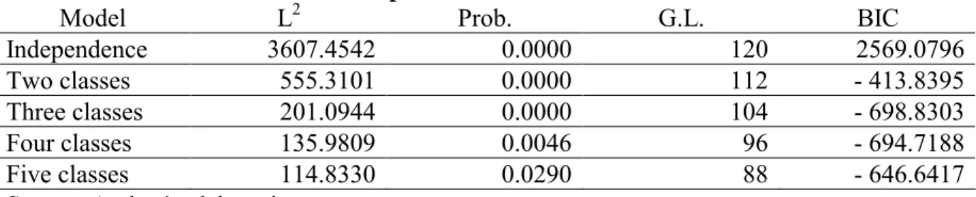
3.3.1 Basic deprivation The analysis of quality fit test of the different models we can considered

shows, firstly, that hypothesis of independence of variables must be rejected.

Table 1. Latent models for basic deprivation

Although it could be argued that none of these models should be accepted, we should recall that, with a large sample size, the addition of small differences causes a large difference and, so the model must be rejected. Therefore, we recommend using the BIC test in such situation.

According to this contrast, we should accept three different groups in the population for basic deprivation.

Table 2. Latent and conditional probabilities for latent basic deprivation

Before commenting every class, we have to say that the variable concerning payment arrears shows “no arrears” as its modal category. The difference lays in probabilities, since the most deprived class has the biggest probability for that category.

The most deprived group is composed by 9.04% of households. These households only can afford eating meat every second day and to possess a telephone. Furthermore, it is estimated that they are not able of facing the rest of needs.

In the other extreme, we have a 56.01% of households, those that can satisfy all the needs. It would be better call them “low deprived households” than “high life style” because we only measure the ability of satisfying needs, not the actual fulfilment or the extent of this satisfaction. For example, the question about new clothes only express the ability of buy them, not their price or quality.

Finally, a 34.95% of the families can satisfy the most of needs, except affording its home adequately warm. Besides, it differs from the class commented before in the conditional probabilities. For this group, the conditional probabilities of inabilities are higher than the ones for the previous class. This group can be called “light deprived households” due to corresponding to an intermediate situation.

3.3.2 Housing Independence of variables is rejected and the hypothesis of three different groups is

accepted again.

Table 3. Latent models for housing deprivation

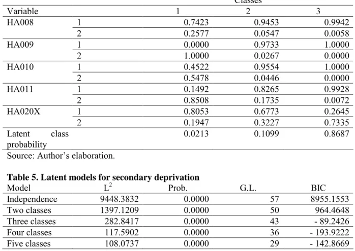
Latent probabilities values show that the most frequent situation of Spanish households is good housing quality. This result agrees with the ones from previous studies on deprivation in Spain already cited.

An 86.87% of households, those that belong to the class 3, have not deprivation in any indicator. They have a separate kitchen, bath or shower, indoor flushing toilet as well as running water. Besides, they live in a free dampness-housing, variable that indicates that this accommodation has not leaks, dampness or rottenness in wooden windows or floors.

On the other hand, it is estimated that the class formed by the most deprived household is very small, almost a 2%. Some households that, except for a separate kitchen, have not the rest of facilities. Even more, the probability of lack of a separate kitchen is the higher in this group. Finally, these households live in homes with leaks, dampness or rottenness in wooden windows or floors.

Table 4. Latent and conditional probabilities for housing deprivation

The last group, though a little greater (a 10.99%), is also small. Its deprivation levels are very similar to levels for the first class since they have all the needs, except the free dampness housing.

Nevertheless, it is more complex to choose the best model. Although, according to BIC test, the four-class model would have to be chosen the model, the best option is selecting the model with three classes.

Table 5. Latent models for secondary deprivation

This decision is based on the exam of conditional and latent probabilities of both models. Two of the classes of the four-class model have some households with similar features, that is, it is estimated the same lack of goods in both. In fact, the amount of latent probabilities is practically identical to the probability for the class that reflects the same phenomenon in the three-class model. They only slightly differ in conditional probabilities values. Since the main goal of this study is to find different groups in population, we consider that it is better to select the three-class model.

Table 6. Latent and conditional probabilities for secondary deprivation

The main feature of this model is the similarity of belonging of each latent class. This phenomenon happens because this deprivation dimension is not related to basic needs or maintenance, but to issues related to life style as being able to afford paying for holidays or having dishwasher.

The smaller group, formed by a 28.24% of households, is the most deprived. Except for the affordability of a colour TV, they cannot face the rest of needs.

On the other hand, a 40.44% of the families belong to the class with smaller deprivation, since can afford all the needs and buying all the goods. Namely, they have or choose not to have them.

The last class, composed by a 31.33%, cannot afford needs concerning holidays and furniture and, though, can afford the possession of durable goods.

3.4 Overall Deprivation

Once different dimensions are analysed, the following step is combine them and to identify different groups in population for this overall definition.

Thus, in this second step we have three variables: HP001 (basic deprivation), HP002 (housing conditions) and HP003 (secondary deprivation) with three categories each one, since the models with three latent classes were selected in each dimension in the first stage of the study.

Again, we seek the existence of subgroups in the population, not a priori established, that have

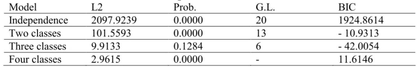
The analysis of the next table shows that there is some relationship between the variables, since the independence hypothesis is rejected. We only accept one model by means BIC test and this model is the one that considers three classes in the population for deprivation.

Table 7. Latent models for overall deprivation

The three determined classes, as we could expect, express the situations shown in the partial studies. Relationship between partial and overall categories is stronger for basic deprivation than secondary. This fact is caused by differences in belonging proportions in each dimension. Since they are very similar in secondary deprivation, there is not a clear differentiation in an intermediate degree of overall multidimensional poverty.

The same reason, belonging proportions, causes that conditional probabilities in housing dimension are higher for “low deprivation” category. We have to remind that the probability of belonging of this category is more than an 85%.

It is estimated that the first group, formed by 12.61% of the families, has a high basic and secondary deprivation levels, more than a 75% in any case. Furthermore, conditional probability estimates for “low deprivation" is nearly zero. Therefore, we can assert that there is an almost perfect identification between high deprivation levels in the overall variable and the respective partial variables.

Table 8. Latent and conditional probabilities for overall deprivation

The analysis of the frequencies assigned to this group shows that basic and secondary dimensions are the most important ones. A high deprivation in at least one of them (category 1) causes the ownership to category 1 of overall deprivation if there is no deprivation in the other one. In fact, a household with high deprivation in both dimensions belongs to “most overall deprived households”, even if it is non-deprived for housing conditions.

The following group, a 39.87% of the families, corresponds to a light or intermediate degree of multidimensional poverty. Again, the analysis of associated frequencies allows proving that the “accommodation” dimension does not affects the ownership to this class, since cells of any category of that dimension appear in this class. Furthermore, the other dimensions are the most important, since this class gather not only their intermediate levels, but also those frequencies composed by the extreme values of both.

Finally, the last and larger class, composed by a 47.52% of households, has the higher probabilities for low deprivation categories in any dimension. For basic dimension, the conditional probability of belonging to minimum overall deprivation category is practically one and the secondary dimension,

presents a smaller probability, though high, a 68.05%. This latter value is due to the greater similarities of belonging probabilities to the latent classes in “secondary needs".

Once the Bayesian assignment process of frequencies to classes is done, we can observed that those cells where the less deprived category for at least one of basic or secondary deprivation appear belong to this class.

In conclusion, the profile of most overall deprived households has as main feature the high levels of deprivation in two of the dimensions, overall, basic and secondary. Furthermore, housing conditions does not discriminate between the different classes of overall deprivation.

On the other side, basic and secondary dimensions are the most important ones. In fact, the presence of the most deprived category of at least one of them caused a household to belong to the group with higher overall deprivation and if appears the highest category of, at least, one it is considered as a non-deprived household. Finally, if both facts happen simultaneously, this household lies in light deprivation group.

4. Conclusions

We have shown that latent class analysis is a useful tool for classifying the households by their deprivation level. This, we overcome the issues derived from using an indirect and multidimensional indicator, income, to measure a multidimensional phenomenon, deprivation. We include a set of direct indicators on living conditions. Besides, considering deprivation as a categorical variable avoid threshold identification problem.

Different dimensions in deprivation have been taken into account: basic needs, secondary needs and housing conditions. Basic deprivation refers to ability for keeping the home adequately warm, buying new clothes, eating meal every second day, having friends or family for drink/dinner, having a car o a telephone and not to have arrears in payments.

The results for 1996 shows that basic needs can be satisfied by the most of households, since only a 9.04% of households suffer a situation where they can afford eating meal every second day and having a telephone.

This fact appears again in housing deprivation where only a 2.13% of households belong to “most deprived” category. That is, a large proportion of households live in an accommodation without problems. Despite this apparently shocking result, we have to recall the kind of households that have been sampled in this panel. Therefore, homeless households are less represented in the sample.

Finally, secondary deprivation is related to life style and, therefore, the proportions are very similar for each category, 28.24%, 31.33% and 40.44%, respectively. Among durable goods, the most deprived category only can afford a colour TV.

Once each deprivation dimension has been studied, they are combined. We found three groups again. Basic and secondary deprivations are the most important variables to decide the belonging to an overall deprivation category. Besides, a 12.61% of households are the most deprived.

1

This is the method proposed by Townsend (1979) and Muffels (1993)

2

Cerioli and Zani (1990), Cheli et al. (1994), Cheli and Lemni (1995), Lemni et al. (1996) and Betti and Cheli (2001).

3

For instante, when a household is asked about running water, there is no difference between lack caused by not affording it and a decided lack.

4

A household has arrears in ordinary payments if it has arrears in, at least, one of the following payments: rent for accommodation, mortgage, utility bills and other loan repayments.

5

A household has this problem if there is one of the following: leaky roof, damp walls or floors and having rot in window frames or floors.

References

Agresti, A. (1990) Categorical data analysis. New York: John Wiley

Anderson, T.W.(1954): On estimation of parameters in latent structure analysis. Psychometrika 19,

1-10.

Atkinson, A.B. (1989) Poverty and social security. London. Harvester Wheatsheaf.

Bartholomew, D.J. (1987) Latent variables models and factor analysis. London. Griffin.

Brandolini, A. and D’Alessio, G. (2000) “Measuring well-being in the functionings space”. 26ª IARIW General Conferene. Krakow.

Bourgignon, F. and Chavrakarty, S.R. (1999) “The measurement of multidimensional poverty” In: Slottje, D.J. Advances in econometrics, income distribution and scientific methodology. Heidelberg.

Physica.

Cantó, O. (1998) Income mobility in Spain: How much is there? Working paper FEDEA EEE 17.

Madrid. FEDEA.

Cantó, O. (2000a) “Income mobility in Spain: How much is there?” Review of Income and Wealth,

46(1), 85-101.

Cantó, O. (2000b) Climbing out of poverty, falling back in: low incomes’ stability in Spain.

Documento de trabajo nº 13, Departamento de Economía Aplicada. Universidad de Vigo.

Clogg, C.C. (1993): Latent class models: recent developments and prospects for the future. In Arminger, G., C.C. Clogg and M.E. Sobel (1993): Handbook of statistical modelling in the social sciences. Plenum, New York.

Dempster, A.P., Laird, N.M., Rubin, D.B. (1977) Maximum likelihood estimation from incomplete data via the EM algorithm. Journal of the Royal Statistical Society B 39:1-38.

Desai, M. and Shah, A. (1988) “An econometric approach to the measurement of poverty”, Oxford Economic Papers, 40(3), 505-522.

Devicenti (2001) Poverty persistence in Britain: a multivariate análisis using the BHPS, 1991-1997.

ISER Working Paper 2001-02. Colchester. University of Essex.

EUROSTAT (2000) European social statistics. Income, poverty and social exclusion. Luxembourg.

Fouarge and Muffels (2000) Persistent poverty in the Netherlands, Germany and the UK. A model-based approach using panel data for the 1990s. European Panel Analysis Group Working Paper nº

15. Colchester. University of Essex.

Goodman, L.A. (1974) “Exploratory latent structure analysis using both identifiable and unidentifiable models”. Biometrika 61: 215-231.

Halleröd, B. (1994) A new approach to the direct consensual measurement of poverty. Social Policy

Hills J., (1998a) “Does income mobility mean that we do not need to worry about poverty?”. In: Atkinson, A.B. y Hills, J. (eds.) Exclusion, employment and opportunity. CASE paper nº 4. London.

CASE – London School of Economics.

Hills, J. (1998b) “What do we mean by reducing lifetime inequality and incresing mobility?”. In

Persistent poverty and lifetime inequality: the evidence. CASE report nº 5. London. CASE-London

School of Economics.

Hirschberg, J.G., Maasoumi, E. and Slottje, J. (1991) “Cluster analysis for measuring welfare and quality of life across countries”. Journal of Econometrics, 50, 131-150.

Layte, R., Maître, B. Nolan, B, and Whelan, C.T. (1999) Income deprivation and economic strain.

European Panel Analysis Group Working Paper nº 5. Colchester. University of Essex.

Layte, R., Maître, B. Nolan, B, and Whelan, C.T. (2000) Explaining levels of deprivation in the European Union. European Panel Analysis Group Working Paper nº 12. Colchester. University of

Essex.

Lazarsfeld, P.F. (1950). “The logical and mathematical foundation of latent structure analysis”. In: Stouffer, S.A. et al. (eds.), Measurement and prediction, 362-472, Princeton. Princeton University

Press.

Lazarsfeld, P.F. and Henry, N.W. (1968) Latent structure analysis. Boston. Houghton Mifflin.

Maasoumi, E. and Nickelsburg, G. (1988) “Multivariate measures of well-being and an analysis of inequality in the Michigan data”. Journal of Business and Economic Statistics, 6, 327-334.

Mack and Lansley (1985) Poor Britain. London. Allen and Urwin.

Martínez, R. and Ruiz-Huerta, J. (1999) “Algunas reflexiones sobre la medición de la pobreza. Una aplicación al caso español”. In: Maravall, J.M. (ed.) Dimensiones de la desigualdad. III Simposio sobre igualdad y distribución de la renta y la riqueza. Vol. 1, 367-428. Madrid. Fundación Argentaria

and Visor Editorial.

Martínez, R. and Ruiz-Huerta, J. (2000) “Income, multiple deprivation and poverty: an empirical analysis using Spanish data”. 26ª IARIW General Conference. Krakow.

Mayer, S.E. and Jencks, C. (1989) “Poverty and the distribution of material resources”. Journal of Human Resources. 21, 88-113.

McCutcheon, A.L.(1987): Latent Class Analysis. Sage, Beverly Hills.

McHugh, R.B. (1956): Efficient estimation and local identification in latent class analysis.

Psychometrika, 21, 331-347.

Muffels, R. and Fouarge, D. (2001) Do European welfare regimes matter in explaining social exclusion? Dynamic analyses of the relationship between income poverty and deprivation: a comparative perspective. ESPE Conference. Athens.

Piachaud, D. (1987) “Problems in the definition and measurement of poverty”. Journal of Social Policy, 16(2), 147-164.

Ram, R. (1982) “Composite indices of physical quality of life, basic needs fulfilment and income. A principal component representation”. Journal of Development Economics, 11, 227-247.

Ringen, S. (1988) “Direct and Indirect Measures of Poverty”, Journal of Social Policy, 17(3),

147-164.

Runciman, W.G. (1966) Relative deprivation and social justice. London. Routledge and Kegan Paul.

Sen, A.K. (1987) The standard of living. Cambridge. Cambridge University Press.

Stevens, A.H. (1994) “Persistence in poverty and welfare: the dynamics of poverty spells: updating Bane and Ellwood”. American Economic Review (Papers and Proceedings), 84: 34-37.

Stevens, A.H. (1999) “Climbing out of poverty, falling back in: measuring the persistence of poverty over multiple spells”. Journal of Human Resources, 3, 557-588.

Townsend, P.(1979) Poverty in the United Kingdom. Harmondsworth. Penguin Books.

Whelan, C.T., Layte, R. y Maître, B. (2001a) What is the scale of multiple deprivation in the European Union?. European Panel Analysis Group Working Paper nº 19. Colchester. University of

Essex.

Whelan, C.T., Layte, R. y Maître, B. (2001b) Persistent deprivation in the European Union. European

Panel Analysis Group Working Paper nº 19. Colchester. University of Essex.

Annex 1. ECHP list of variables

HF003

Can the household afford keeping its home

adequately warm

HF004

Can the household afford paying for holiday

HF005

Can the household afford replacing worn-out

furniture

HF006

Can the household afford buy new clothes

HF007

Can the household afford eating meal every

second day

HF008

Can the household afford having friends or

family for drink/dinner

HF009

Has the household been unable to pay

scheduled rent for accommodation during the

past 12 months

HF010

Has the household been unable to pay

scheduled mortgage payments during the past

12 months

HF011

Has the household been unable to pay

scheduled utility bills during the past 12

months

HF012

Has the household been unable to pay other

loan repayments rent for accommodation

during the past 12 months

HA008

Does the dwelling have separate kitchen

HA009

Does the dwelling have bath or shower

HA010

Does the dwelling have indoor flushing toilet

HA011

Does the dwelling have running water

HA012

Does the dwelling have leaky roof

HA013

Does the dwelling have damp walls or floors

HA014

Does the dwelling have rot in window frames

or floors

HB001

Possession of a car

HB002

Possession of a colour TV

HB003

Possession of a VCR

HB004

Possession of a micro wave

HB005

Possession of a dishwasher

Table 1. Latent models for basic deprivation

Model L

2

Prob. G.L. BIC

Independence 3607.4542 0.0000

120

2569.0796

Two classes

555.3101

0.0000

112

- 413.8395

Three classes

201.0944

0.0000

104

- 698.8303

Four classes

135.9809

0.0046

96

- 694.7188

Five classes

114.8330

0.0290

88

- 646.6417

Source: Author’s elaboration.

Table 2. Latent and conditional probabilities for latent basic deprivation

Classes

Variables

1 2 3

HF003

1

0.0724

0.0935

0.6675

2

0.9276

0.9065

0.3325

HF006 1

0.2234

0.8574 0.9862

2

0.7766

0.1426

0.0138

HF007 1

0.6117

0.9796 0.9999

2

0.3883

0.0204

0.0001

HF008 1

0.1252

0.7781 0.9755

2

0.8748

0.2219

0.0245

HF010X 1

0.3172

0.1248 0.0283

2

0.6828

0.8752

0.9717

HB001 1

0.4943

0.7196 0.9636

2

0.5057

0.2804 0.0364

HB006 1

0.6432

0.8136 0.9944

2

0.3568

0.1864

0.0056

Latent class

probability

0.0904

0.3495

0.5601

Source: Author’s elaboration.

Table 3. Latent models for housing deprivation

Model L

2

Prob. G.L. BIC

Independence 1380.5271 0.0000

26

1155.5459

Two classes

78.2951

0.0000

20

- 94.7674

Three classes

22.7893

0.0638

14

- 98.3544

Four classes

22.7890

0.0036

8

- 46.4359

Five classes

19.5475

0.0001

2

2.2413

Table 4. Latent and conditional probabilities for housing deprivation

Classes

Variable 1 2 3

HA008 1

0.7423

0.9453 0.9942

2

0.2577

0.0547

0.0058

HA009 1

0.0000

0.9733 1.0000

2

1.0000

0.0267

0.0000

HA010 1

0.4522

0.9554 1.0000

2

0.5478

0.0446

0.0000

HA011 1

0.1492

0.8265 0.9928

2

0.8508

0.1735

0.0072

HA020X 1

0.8053

0.6773 0.2645

2

0.1947

0.3227

0.7335

Latent class

probability

0.0213

0.1099

0.8687

Source: Author’s elaboration.

Table 5. Latent models for secondary deprivation

Model L

2

Prob. G.L. BIC

Independence 9448.3832 0.0000

57

8955.1553

Two classes

1397.1209

0.0000

50

964.4648

Three classes

282.8417

0.0000

43

- 89.2426

Four classes

117.5902

0.0000

36

- 193.9222

Five classes

108.0737

0.0000

29

- 142.8669

Source: Author’s elaboration.

Table 6. Latent and conditional probabilities for secondary deprivation

Classes

Variables

1 2 3

HF004 1

0.1213

0.1787 0.9089

2

0.8787

0.8213

0.0911

HF005 1

0.1047

0.1092 0.7865

2

0.8953

0.8908

0.2135

HB002 1

0.9458

0.9959 0.9999

2

0.0542

0.0041

0.0001

HB003 1

0.4162

0.9482 0.9967

2

0.5838

0.0518

0.0033

HB004 1

0.0555

0.9762 0.9962

2

0.9945

0.0238

0.0038

HB005 1

0.0338

0.7765 0.9685

2

0.9662

0.2235

0.0315

Latent class

probability

0.2824

0.3133

0.4044

Table 7. Latent models for overall deprivation

Model L2

Prob. G.L. BIC

Independence 2097.9239

0.0000

20

1924.8614

Two classes

101.5593

0.0000

13

- 10.9313

Three

classes

9.9133 0.1284 6

-

42.0054

Four

classes

2.9615 0.0000 -

11.6146

Source: Author’s elaboration.

Table 8. Latent and conditional probabilities for overall deprivation

Classes

Variables

1 2 3

HP001 1

0.7659 0.1357 0.0001

2 0.2341

0.3428

0.0293

3 0.0001

0.5215

0.9707

HP002 1

0.1124 0.0103 0.0056

2 0.1399

0.0413

0.0161

3 0.7477

0.9484

0.9783

HP003 1

0.8487 0.4543 0.0002

2 0.1513

0.4967

0.3194

3 0.0001

0.0490

0.6805

Latent class

probability

0.1261

0.3987

0.4752

Figure 1. Strategies for measuring deprivation (Brandolini and D'Alessio, 2000)

Item-by-item analysis Suplementation strategy

Vector dominance Sequential dominance Multivariate techniques Multidimensional inequality indexes Non-aggregative strategies Well-being indicator Equivalence scales Aggregative strategies Comprehensive analysis

Item-by-item analysis Suplementation strategy

Vector dominance Sequential dominance Multivariate techniques Multidimensional inequality indexes Non-aggregative strategies Well-being indicator Equivalence scales Aggregative strategies Comprehensive analysis

IRISS-C/I is currently supported by the European Community under the Transnational Access to Major Research Infrastructuresaction of the Improving the

Human Research Potential and the Socio-Economic Knowledge Baseprogramme (5th

framework programme) [contract HPRI-CT-2001-00128]

Please refer to this document as