Volume 71, Number 240, Pages 1781–1797 S 0025-5718(01)01382-5
Article electronically published on November 28, 2001
NUMERICAL CALCULATION
OF THE DENSITY OF PRIME NUMBERS WITH A GIVEN LEAST PRIMITIVE ROOT
A. PASZKIEWICZ AND A. SCHINZEL
Abstract. In this paper the densitiesD(i) of prime numbersp having the
least primitive rootg(p) = i, where iis equal to one of the initial positive integers less than 32, have been numerically calculated. The computations were carried out under the assumption of the Generalised Riemann Hypothesis. The results of these computations were compared with the results of numerical frequency estimations.
1. An outline of the method of computation
Letg(p) denote the least primitive root modulopandD(i) the density of prime numbers with the least primitive root equal toi, that is
D(i) = lim x→∞π(x) −1 X p≤x g(p)=i 1.
In [3] Elliott and Murata gave the formula
D(i) =X
M
(−1)|M|−1AM,
(1)
where M runs over all the subsets of the set {2,3, . . . , i} containingi. HereAM
denotes the conjectural density of primes psuch that eachai ∈ M is a primitive root modulop, expressed by the formula in Lemma 11.5, page 140 of Matthews [4]:
AM =Y p (1−c(p)) X a∈G(a1,...,an) ω(a)f(a), (2)
where M ={a1, . . . , an} andG(a1, . . . , an} is the set of squarefree integers of the form a =κ(aε11 , . . . , aεn
n )≡ 1(mod 4), εi = 0,1, ω(a) = (−1) P
iεi and κ(b) is the squarefree part of the numberb
f(b) =µ(b)Y
p|b c(p) 1−c(p).
Herec(p) is the natural density of the set of primes{q:q≡1(modp),q-a1, . . . , an, and at least one of the numbersa1, . . . , an is apth power residue moduloq}.
Received by the editor November 29, 1999 and, in revised form, December 26, 2000. 2000Mathematics Subject Classification. Primary 11Y16; Secondary 11A07, 11M26.
Key words and phrases. Prime, generators, primitive roots, extended Riemann hypothesis.
c
Formula (2) is based on the assumption that ifaεi
1, . . . , aεnn=b2, thenS=
P
iεi
is even. IfS is odd, thenAM = 0. There is a factor 1/2n missing in (1.4) page 114
of Matthews [4], and this error is repeated in the paper of Elliott and Murata. In [3] Elliott and Murata derived formulas for the density of prime numbers whose least primitive roots are the initial natural numbers 2,3,5,6 and 7. They are as follows: D(2) = ∆, D(3) = ∆1−∆2, D(5) = 20 19∆1− 200 91 ∆2+ 500 439∆3, D(6) = ∆1− 282 91∆2+ 1000 439∆3, D(7) = ∆1− 4 + 9 91+ 5 281 ∆2+ 6 +183 439+ 4826 67585+ 147193 29669815 ∆3 − 3 + 1107 2131+ 71825 1290197+ 26503425 2749409807 ∆4, where the initial ∆i (i= 1,2,3,4) are
∆1= Y p≥2 1− 1 p(p−1) ,Artin’s constant, ∆2= Y p≥2 1− 2 p(p−1)+ 1 p2(p−1) , ∆3= Y p≥2 1− 3 p(p−1)+ 3 p2(p−1) − 1 p3(p−1) , ∆4= Y p≥2 1− 4 p(p−1)+ 6 p2(p−1) − 4 p3(p−1)+ 1 p4(p−1) .
The calculation of the successive values ofD(i) is illustrated with an example for
i= 10. According to (1),
D(10) =X
M
(−1)|M|−1AM,
where M runs over all the subsets of the set {2,3,5,6,7,10} containing 10 (from the set of all natural numbers≤10, we remove the powers 1,4,8,9, which can never be least primitive roots). Observe that if M containsa, b and ab, then AM = 0, because ifa, bare primitive roots forp, thenab is not. Therefore,
D(10) =A{10}−A{2,10}−A{3,10}−A{5,10}−A{6,10} −A{7,10}+A{2,3,10}+A{2,6,10}+A{2,7,10} +A{3,5,10}+A{3,6,10}+A{3,7,10}+A{5,6,10} +A{5,7,10}+A{6,7,10}−A{2,3,7,10}−A{2,6,7,10} −A{3,5,7,10}−A{3,6,7,10}−A{5,6,7,10} −A{3,5,6,10}+A{3,5,6,7,10}.
Now, for each of the 22 setsM, listed above we calculatec(p), which we denote by
multiplicatively independent (that is they do not satisfy any relation of the form
aα11 a α2
2 · · ·aαnn= 1, whereαi (i= 1,2, . . . , n) are integers not all equal to 0), then
c(p, M) = 1 p−1 1− 1−1 p |M|! ; (3) hence, Y p≥2 (1−c(p, M)) = ∆|M|.
The assumption of the multiplicative independence of the elements holds for all the sets listed above except for{3,5,6,10}and{3,5,6,7,10}(we have 3·5−1·6−1·10 = 1). In order to apply Matthews’s formula (2) we compute the sum
S(M) = 1 X ε1=0 a=κ(aε1 1 ···aεnn ) · · ·≡ 1 X εn=0 1(mod 4) (−1)Piεif(|a|, M),
where the additional argument of the functionf was added in order to avoid am-biguity, e.g., forM ={10}, S(M) =f(1, M) = 1, forM ={2,10}, S(M) =f(1, M) +f(5, M) = 1− c(5, M) 1−c(5, M) = 1− 9 91 = 82 91. The first summand corresponds to the choiceε1=ε2= 0; the second to the choice ε1 = ε2 = 1, etc. The calculation of the values of the coefficients AM for the remaining sets M proceeds similarly up to the setM ={5,6,7,10}inclusive. For
M ={5,6,7,10}we have S(M) =f(1, M)−f(5, M) +f(21, M)−f(105, M) = 1 + c(5, M) 1−c(5, M)+ c(3, M) 1−c(3, M)· c(7, M) 1−c(7, M) + c(5, M) 1−c(5, M)· c(3, M) 1−c(3, M)· c(7, M) 1−c(7, M).
The first summand corresponds to the choiceε1=ε2=ε3=ε4= 0; the second to the choiceε1 = 1, ε2 =ε3=ε4 = 0; the third toε1 =ε2=ε3 =ε4= 1; and the fourth to ε1= 0, ε2=ε3=ε4= 1.
It remains to consider two special setsM1={3,5,6,10}andM2={3,5,6,7,10}. For these sets the formula (3) is not valid and is replaced with
c(p, M1) = 4 p(p−1) − 6 p2(p−1) + 3 p3(p−1), S(M1) = 2f(1, M1)−2f(5, M1) = 2 + 2 c(5, M1) 1−c(5, M1) .
The first summand corresponds to the choiceε1=ε3=ε4=ε2; the second to the choiceε1=ε3=ε46=ε2: c(p, M2) = 5 p(p−1) − 10 p2(p−1) + 9 p3(p−1) − 3 p4(p−1); S(M2) = 2f(1, M2)−2f(5, M2) + 2f(21, M2)−2f(105, M2) = 2 + 2 c(5, M2) 1−c(5, M2) + 2 c(3, M2) 1−c(3, M2)· c(7, M2) 1−c(7, M2) + 2 c(3, M2) 1−c(3, M2)· c(5, M2) 1−c(5, M2)· c(7, M2) 1−c(7, M2) .
The first summand corresponds to the choiceε1=ε3 =ε3,ε4 =ε1+ε3, ε5=ε3; the second to the chioce ε1 = ε3 6= ε2, ε4 = ε1+ε3, ε5 = ε3; the third to the choiceε2=ε3 6=ε1,ε4=ε1+ε3, ε5=ε3; the fourth to the choice ε1=ε2 6=ε3, ε4=ε1+ε3,ε5=ε3.
Proceeding in this way, we can calculate densitiesD(i) for any positive integer
i. Beyondi= 10, the derivation of formulas forD(i) ceases to make sense due to their length. However, the use of a computer makes it possible to extend the com-putations to some extent. In this paper, by designing an algorithm corresponding to the computational process described above, we computed the values ofD(i) for all positive integersi <32, which are not powers of integers.
2. Results of numerical computations
The following numerical investigations were carried out:
• The densities D(i) of prime numbers p having the least primitive rootg(p) equal toiwere calculated; the results are illustrated in Table 3.
• For every prime numberp <4·1010, the value of its least primitive root was determined.
• The computed densities of prime numbers with given least primitive roots were compared with numerical frequency estimates; the respective values are shown side by side in Table 3.
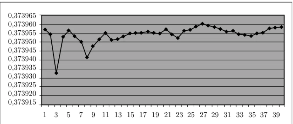
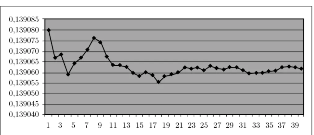
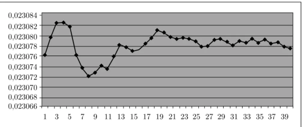
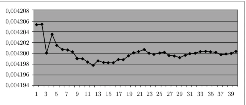
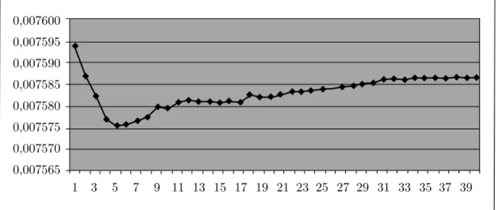
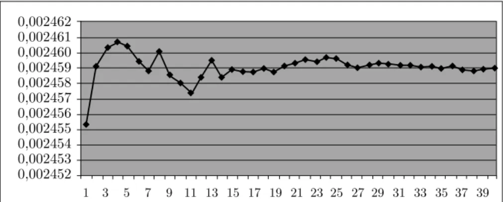
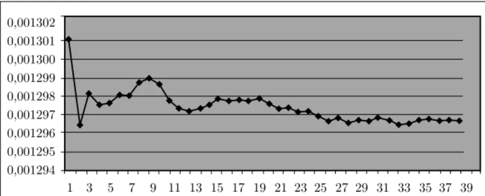
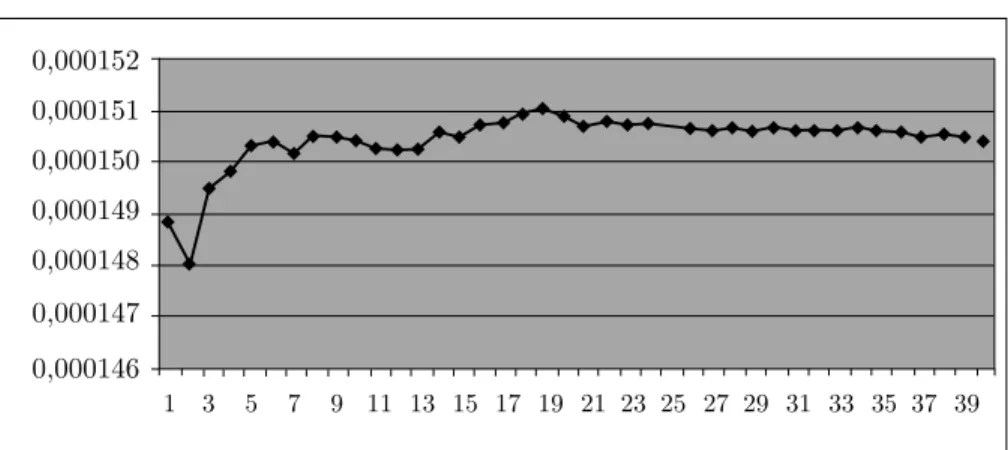
• The graphs of densitiesD(i) for initial values ofiwere prepared and tabulated with step equal to 109, the behaviour of the frequencies of prime numbers with a given least primitive root are illustrated in Figures 1–24. From the figures it may be concluded that the densitiesD(i) are very stable. Oscillations have limited amplitude and a tendency to damp out.
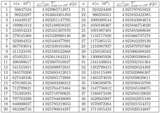
• A graph of the average value of the least primitive root of prime numbers not exceeding 4·1010 was prepared (Figure 25) and tabulated with a step equal to 109 (Table 1).
• The growth rate of the least primitive root of a prime number was numerically investigated (see Table 2). The valueg(p) of the least primitive root of a prime number p is well majorised by a second degree polynomial of the natural logarithm of p, which agrees with the conjecture by E. Bach [1] about the least primitive prime roots modulo a prime number.
All computations were performed with the aid of more than ten desktop IBM PC computers from Pentium 100 to Pentium III 500 during their idle time. The computations lasted approximately one year. The computational procedures (with some small exceptions) were written in a high level language in order to minimise the risk of programming error. Most of the results were verified using popular
numerical packages, e.g., MAPLE, GP/PARI. The verification required more time than the actual computations. For checking the number of primes generated, we used Mapes’s algorithm, which was found to be the most computationally effective within the range of computations performed.
0,373965 0,373960 0,373955 0,373950 0,373945 0,373940 0,373935 0,373930 0,373925 0,373920 0,373915 1 3 5 7 9 11 13 15 17 19 21 23 25 27 29 31 33 35 37 39
Figure 1. The densityD(2) of prime numbers with the least
prim-itive root equal to 2
0,226620 0,226615 0,226610 0,226605 0,226600 0,226595 0,226590 0,226585 0,226580 0,226575 1 3 5 7 9 11 13 15 17 19 21 23 25 27 29 31 33 35 37 39
Figure 2. The densityD(3) of prime numbers with the least
0,139085 0,139080 0,139075 0,139070 0,139065 0,139060 0,139055 0,139050 0,139045 0,139040 1 3 5 7 9 11 13 15 17 19 21 23 25 27 29 31 33 35 37 39
Figure 3. The densityD(5) of prime numbers with the least
prim-itive root equal to 5
0,055905 0,055900 0,055895 0,055890 0,055885 0,055880 0,055875 0,055870 0,055865 0,055860 0,055855 1 3 5 7 9 11 13 15 17 19 21 23 25 27 29 31 33 35 37 39
Figure 4. The densityD(6) of prime numbers with the least
prim-itive root equal to 6
1 3 5 7 9 11 13 15 17 19 21 23 25 27 29 31 33 35 37 39 0,068720 0,068715 0,068710 0,068705 0,068700 0,068695
Figure 5. The densityD(7) of prime numbers with the least
1 3 5 7 9 11 13 15 17 19 21 23 25 27 29 31 33 35 37 39 0,023084 0,023082 0,023080 0,023078 0,023076 0,023074 0,023072 0,023070 0,023068 0,023066
Figure 6. The density D(10) of prime numbers with the least
primitive root equal to 10 0,037260 0,037255 0,037250 0,037245 0,037240 0,037235 0,037230 0,037225 0,037220 1 3 5 7 9 11 13 15 17 19 21 23 25 27 29 31 33 35 37 39
Figure 7. The density D(11) of prime numbers with the least
primitive root equal to 11
0,003285 0,003280 0,003275 0,003270 0,003265 0,003260 0,003255 0,003250 1 3 5 7 9 11 13 15 17 19 21 23 25 27 29 31 33 35 37 39
Figure 8. The density D(12) of prime numbers with the least
0,023245 0,023240 0,023235 0,023230 0,023225 0,023220 0,023215 0,023210 0,023205 0,023200 1 3 5 7 9 11 13 15 17 19 21 23 25 27 29 31 33 35 37 39
Figure 9. The density D(13) of prime numbers with the least
primitive root equal to 13 0,008273 0,008272 0,008271 0,008270 0,008269 0,008268 0,008267 0,008266 0,008265 0,008264 0,008263 1 3 5 7 9 11 13 15 17 19 21 23 25 27 29 31 33 35 37 39
Figure 10. The density D(14) of prime numbers with the least
primitive root equal to 14 0,004208 0,004206 0,004204 0,004202 0,004200 0,004198 0,004196 0,004194 1 3 5 7 9 11 13 15 17 19 21 23 25 27 29 31 33 35 37 39
Figure 11. The density D(15) of prime numbers with the least
0,011575 0,011570 0,011565 0,011560 0,011555 0,011550 1 3 5 7 9 11 13 15 17 19 21 23 25 27 29 31 33 35 37 39
Figure 12. The density D(17) of prime numbers with the least
primitive root equal to 17
0,000406 0,000404 0,000402 0,000400 0,000398 0,000396 0,000394 1 3 5 7 9 11 13 15 17 19 21 23 25 27 29 31 33 35 37 39
Figure 13. The density D(18) of prime numbers with the least
primitive root equal to 18
0,007600 0,007595 0,007590 0,007585 0,007580 0,007575 0,007570 0,007565 1 3 5 7 9 11 13 15 17 19 21 23 25 27 29 31 33 35 37 39
Figure 14. The density D(19) of prime numbers with the least
0,0001690fl 0,0001685fl 0,0001680fl 0,0001675fl 0,0001670fl 0,0001665fl 0,0001660fl 0,0001655 1 3 5 7 9 11 13 15 17 19 21 23 25 27 29 31 33 35 37 39
Figure 15. The density D(20) of prime numbers with the least
primitive root equal to 20
1 3 5 7 9 11 13 15 17 19 21 23 25 27 29 31 33 35 37 39 0,001603 0,001602 0,001601 0,001600 0,001599 0,001598 0,001597 0,001596
Figure 16. The density D(21) of prime numbers with the least
primitive root equal to 21
0,002462 0,002461 0,002460 0,002459 0,002458 0,002457 0,002456 0,002455 0,002454 0,002453 0,002452 1 3 5 7 9 11 13 15 17 19 21 23 25 27 29 31 33 35 37 39
Figure 17. The density D(22) of prime numbers with the least
0,003875 0,003874 0,003873 0,003872 0,003871 0,003870 0,003869 0,003868 1 3 5 7 9 11 13 15 17 19 21 23 25 27 29 31 33 35 37 39
Figure 18. The density D(23) of prime numbers with the least
primitive root equal to 23
0,0000231 0,0000230 0,0000229 0,0000228 0,0000227 0,0000226 0,0000225 0,0000224 0,0000223 0,0000222 1 3 5 7 9 11 13 15 17 19 21 23 25 27 29 31 33 35 37 39
Figure 19. The density D(24) of prime numbers with the least
primitive root equal to 24 0,001302 0,001301 0,001300 0,001299 0,001298 0,001297 0,001296 0,001295 0,001294 1 3 5 7 9 11 13 15 17 19 21 23 25 27 29 31 33 35 37 39
Figure 20. The density D(26) of prime numbers with the least
1 3 5 7 9 11 13 15 17 19 21 23 25 27 29 31 33 35 37 39 0,000152 0,000151 0,000150 0,000149 0,000148 0,000147 0,000146
Figure 21. The density D(28) of prime numbers with the least
primitive root equal to 28 0,002207 0,002206 0,002205 0,002204 0,002203 0,002202 1 3 5 7 9 11 13 15 17 19 21 23 25 27 29 31 33 35 37 39
Figure 22. The density D(29) of prime numbers with the least
primitive root equal to 29
0,0001055 0,0001050 0,0001045 0,0001040 0,0001035 0,0001030 1 3 5 7 9 11 13 15 17 19 21 23 25 27 29 31 33 35 37 39
Figure 23. The density D(30) of prime numbers with the least
0,001483 0,001482 0,001481 0,001480 0,001479 0,001478 0,001477 0,001476 1 3 5 7 9 11 13 15 17 19 21 23 25 27 29 31 33 35 37 39
Figure 24. The density D(31) of prime numbers with the least
primitive root equal to 31
1 3 5 7 9 11 13 15 17 19 21 23 25 27 29 31 33 35 37 39 4,9265 4,9260 4,9255 4,9250 4,9245 4,9240 4,9235
Figure 25. The average value of the least primitive root. The
Table 1. The average value of the least primitive root n π(n·109) 1 π(n·109) P p<n·109g(p) n π(n·10 9 ) 1 π(n·109) P p<n·109g(p) 1 50847534 4.923965712871 21 924324489 4.925797855823 2 98222287 4.924663401493 22 966358351 4.925832422385 3 144449537 4.925051147795 23 1008309544 4.925843984674 4 189961812 4.925188058325 24 1050186367 4.925846754020 5 234954223 4.925341307870 25 1091987405 4.925855088048 6 279545368 4.925330900136 26 1133717820 4.925866737278 7 323804352 4.925440477091 27 1175385155 4.925842229139 8 367783654 4.925509101064 28 1216987937 4.925879767368 9 411523195 4.925580522868 29 1258528162 4.925900388393 10 455052511 4.925611642211 30 1300005926 4.925903390845 11 498388617 4.925607016827 31 1341430624 4.925932161364 12 541555851 4.925698972831 32 1382799415 4.925928524492 13 584570200 4.925693412013 33 1424115489 4.925920066307 14 627440336 4.925695173988 34 1465374659 4.925939629611 15 670180516 4.925693396312 35 1506589876 4.925939416709 16 712799821 4.925704473484 36 1547756812 4.925945180075 17 755305935 4.925719780025 37 1588873108 4.925950159639 18 797703398 4.925784038089 38 1629945987 4.925942955189 19 840000027 4.925795219053 39 1670972264 4.925921554372 20 882206716 4.925790644287 40 1711955433 4.925920544687
Table 2. The growth rate of the least primitive root modulo a
prime number. The range of computations covers all prime num-bers less than 4·1010.
g(p) p ln(g(pp)) lng2(p(p)) g(p) ln3(p) 3−γg(p) ln(p)(ln ln(p))2 3 7 1.541695 0.792274 0.407148 1.953083 5 23 1.594644 0.508578 0.162200 0.685570 6 41 1.615695 0.435078 0.117159 0.527004 7 71 1.642159 0.385241 0.090375 0.438590 19 191 3.617481 0.688745 0.131132 0.738260 21 409 3.492017 0.580675 0.096558 0.609157 23 2161 2.995444 0.390116 0.050807 0.404762 31 5881 3.571641 0.411504 0.047411 0.429429 37 37761 3.510758 0.333119 0.031608 0.355390 38 55441 3.478873 0.318488 0.029157 0.341698 44 71761 3.935213 0.351952 0.031477 0.379080 69 110881 5.939973 0.511352 0.044020 0.554523 73 760321 5.390837 0.398097 0.029398 0.445765 94 5109721 6.085459 0.393966 0.025504 0.455971 97 17551561 5.815119 0.348614 0.020899 0.412241 101 29418841 5.873067 0.341514 0.019858 0.407471 107 33358081 6.176826 0.356571 0.020583 0.426360 111 45024841 6.298685 0.357418 0.020281 0.429585 113 90441961 6.168048 0.336679 0.018377 0.409520 127 184254841 6.673031 0.350624 0.018423 0.431661 137 324013369 6.991117 0.356757 0.018205 0.443395 151 831143041 7.352113 0.357970 0.017429 0.451916 164 1685283601 7.719390 0.363347 0.017102 0.464042 179 6064561441 7.946469 0.352773 0.015660 0.459908 194 7111268641 8.551926 0.376986 0.016618 0.492719 197 9470788801 8.575852 0.373326 0.016251 0.490148 227 28725635761 9.426496 0.391448 0.016255 0.522907
Table 3. The frequencies of occurrence of prime numbers with
a given least primitive root. D(i) denotes the frequency of prime numbers with the least primitive root equal to i, calculated with the aid of theoretical considerations.
i D(i) π(1a)Pp<a,g(p)=i (a=4·1010) 1 2 0.373955 0.3739585 3 0.226606 0.2266042 5 0.139065 0.1390616 6 0.055881 0.0558824 7 0.068702 0.0687077 10 0.023074 0.0230774 11 0.037238 0.0372384 12 0.003263 0.0032617 13 0.023229 0.0232346 14 0.008270 0.0082698 15 0.004200 0.0042004 17 0.011568 0.0115673 18 0.000404 0.0004047 19 0.007586 0.0075864 20 0.000168 0.0001687 21 0.001600 0.0015989 22 0.002459 0.0024589 23 0.003873 0.0038720 24 0.000022 0.0000227 26 0.001297 0.0012966 28 0.000150 0.0001503 29 0.002203 0.0022049 30 0.000104 0.0001050 31 0.001479 0.0014784
3. Acknowledgments
The referee informed us that in the Ph.D. thesis of Bob Buttsworth, University of Queensland 1983 [2], the formula for D(i) is transformed using finite difference methods, into a form which allows one to prove thatD(i) is positive if i is not a perfect power, for which we are grateful.
The first author was technically supported during computations by the grant of Polish Committee for Scientific Research Nr. 8 T11 D 011 12.
References
1. E. Bach,Comments on search procedures for primitive roots, Math. Comp.66(1997), 1719– 1727. MR98a:11187
2. R. N. Buttsworth,A general theory of inclusion-exclusion with application to the least primitive root problem, and other density question, Ph.D. Thesis, University of Queensland, Queensland, 1983.
3. P.D.T.A. Elliott, L. Murata,On the average of the least primitive root modulop, J. London Math. Soc. (2)56(1997), 435-454. MR98m:11094
4. K. R. Matthews, A generalisation of Artin’s conjecture for primitive roots, Acta Arith.29 (1976), 113–146. MR53:313
Warsaw University of Technology, Institute of Telecommunications, Division of Telecommunications Fundamental, ul. Nowowiejska 15/19, 00-665 Warsaw, Poland
E-mail address: [email protected]
Institute of Mathematics, Polish Academy of Sciences, ul. ´Sniadeckich 8, 00-950 War-saw, Poland