Bayesian Value-at-Risk for a Portfolio: Multi- and Univariate Approaches Using MSF-SBEKK Models

(1)

Bayesian Value-at-Risk for a Portfolio:

Multi- and Univariate Approaches Using

MSF-SBEKK Models

Jacek Osiewalski

∗

, Anna Pajor

†

Submitted: 7.12.2010, Accepted: 31.03.2011

Abstract

The s-period ahead Value-at-Risk (VaR) for a portfolio of dimension n

is considered and its Bayesian analysis is discussed. The VaR assessment

can be based either on the n-variate predictive distribution of future returns

on individual assets, or on the univariate Bayesian model for the portfolio

value (or the return on portfolio). In both cases Bayesian VaR takes into

account parameter uncertainty and non-linear relationship between ordinary and logarithmic returns. In the case of a large portfolio, the applicability of the

n-variate approach to Bayesian VaR depends on the form of the statistical model

for asset prices. We use then-variate type I MSF-SBEKK(1,1) volatility model

proposed specially to cope with largen. We compare empirical results obtained

using this multivariate approach and the much simpler univariate approach based on modelling volatility of the value of a given portfolio.

Keywords: Bayesian econometrics, risk analysis, multivariate GARCH processes, multivariate SV processes, hybrid SV-GARCH models

JEL Classification: C11, C22, C32, C53, G17

∗_{Cracow University of Economics, e-mail: [email protected]} †_{Cracow University of Economics, e-mail: [email protected]}

253 J. Osiewalski, A. Pajor

(2)

Jacek Osiewalski, Anna Pajor

1 Introduction

Investors calculate Value-at-Risk (VaR) for their portfolios, which are usually quite large. VaR means the loss (of the portfolio value) that would be reached or exceeded with a given probabilityα(usually 0.05 or smaller) over a certain time horizon (most often from 1 to 10 days). Despite theoretical discussions (see Artzner, Delbaen, Eber, Heath 1999), VaR has become the standard measure of market risk used both by financial institutions and by their regulators; see Engle and Manganelli (2004). VaR is a characteristic of the distribution of the future portfolio value (conditional on historical data on asset prices) and is closely related to its left tail. In practice, this probability distribution is unknown and is replaced by a statistical (sampling) model, that is a family of probability distributions; the data are used to choose its most appropriate element, which leads to the estimate of VaR. More traditional approaches to the assessment of VaR are based on parametric statistical models (usually from the GARCH family), which describe the whole distribution of future returns. The recently popular CAViaR approach (based on quantile regression) directly focuses on theα-quantile modelled non-parametrically; see Engle and Manganelli (2004). In this paper we discuss and compare VaR assessment based on multi- and univariate parametric models. Multivariate approach is much more difficult, as it explicitly takes into account the full conditional covariance structure of asset prices: individual volatilities and correlations. On the other hand, VaR requires only the distribution of the future value of the portfolio; it can be derived using a univariate model for the historical values of the portfolio. Such an univariate approach is much simpler, since it does not need specifying the covariance structure of the assets.

In our comparison we refer to parametric models and use the Bayesian statistical paradigm that unifies the theory and practice of VaR. Within this paradigm, the parametric sampling models together with prior distributions can be used as building blocks for the unique predictive distribution of the future portfolio value. The predictive distribution automatically takes into account uncertainty about the parameters of the statistical model used to describe historical data. Also, specification (model) uncertainty can easily be incorporated using Bayesian pooling ("model averaging"), not considered in this paper. The predictive Bayesian formulation of VaR will be called Bayesian VaR.

The focus on the (left) tail of the predictive distribution requires (as its building block) a statistical model that is capable of estimating and forecasting the chances of extreme or outlying observations. The practical usefulness of Bayesian VaR depends on particular models under consideration as well as on numerical methods used in analysing the predictive distribution. Most of multivariate specifications in financial econometrics either belong to the MGARCH (Multivariate GARCH) or MSV (Multivariate Stochastic Volatility) classes or are based on copulas; see Bauwens, Laurent, Rombouts (2006), Tsay (2005). These models are difficult to estimate; only a few of them could be practical tools for large portfolios. A solution to the problem of simple, parsimonious multivariate volatility modelling is a hybrid model proposed by

(3)

Osiewalski (2009); see also Osiewalski and Pajor (2009). This hybrid model is based on scalar BEKK (SBEKK) correlation structure and the simplest MSV specification, the Multiplicative Stochastic Factor (MSF) model. Here we use the MSF-SBEKK type I model for portfolios of dimension n= 34 and n= 50. In order to make the univariate model of portfolio value comparable to the n-variate model of individual assets, we consider the univariate specification obtained from the MSF-SBEKK one by takingn= 1.

In the next section we discuss basic notions and introduce notation. In section 3 we present the foundations of Bayesian VaR. Section 4 is devoted to our models proposed for the assessment of VaR. Sections 5 and 6 contain empirical results for portfolios of dimension 34 and 50, respectively. Section 7 concludes.

2 Portfolio VaR - concepts, notation, modelling

approaches

Consider a portfolio kept at present time (T) and consisting ofn assets;ai denotes

the number of units of asset ipossessed now and St,i is the price of asseti at time

t (St,i>0, ai >0 for i = 1, . . . , n), thus Wt =

n

P

i=1

aiSt,i is the timet value of this

portfolio. Thes-period return rate on the portfolio is:

R∗_t_:_t₊_s= (Wt+s−Wt) Wt = n X i=1 ωt,iRt:t+s,i, where Rt:t+s,i = (St+s,i−St,i)

St,i is thes-period return rate on asset i and ωt,i =

aiSt,i

Wt is the share of asset i in the time t portfolio value. For most results ai > 0 is not

required (short sale is allowed), only Wt>0 has to be assumed. Note that the sum

ofωt,i over the assets (i= 1, . . . , n) is always 1 by construction.

Assume that we observe the n-variate time series of individual return rates for

t = 1, . . . , T and we are interested in forecasting R∗_T_:_T₊_s, thes-period ahead return

on the portfolio kept at timeT. ForecastingR∗_T_:_T₊_sis closely related to the definition of V aRT:T+s, the s-period ahead Value-at-Risk of the portfolio. IfΨT denotes the

current and past asset prices, then V aRT:T+s(α) for a given probability level α is

defined by the following equality:

P r{WT+s≤WT −V aRT:T+s(α)|ΨT}=α, (1)

which can be written as

P r R_T∗_:_T₊_s≤−V aRT:T+s(α) WT |ΨT =α. (2)

Under any continuous distribution, the relative s-period ahead Value-at-Risk (corresponding to some fixed, small α) is the absolute value of the α-quantile of

(4)

the conditional distribution of the s-period ahead return on the portfolio, given the current and past asset prices.

The ordinary return rates Rt:t+s,i > −1 are rarely used in statistical modelling of

asset prices and returns. Instead, the logarithmic return ratesrt+1,i= ln

_S

t+1,i

St,i

= = ln (Rt:t+s,i+ 1)are the quantities being modelled; they can take any real value and

easily aggregate over time:

rt:t+s,i= ln (Rt:t+s,i+ 1) = ln _S t+s,i St,i = s X j=1 ln _S t+j,i St+j−1,i = s X j=1 rt+j,i

SinceRt:t+s,i+ 1 = exp s P j=1 rt+j,i ! andR∗ t:t+s= n P i=1

ωt,iRt:t+s,i, we can rewrite (1)

as P r    −1 + n X i=1 ωT ,iexp   s X j=1 rT+j,i  ≤ − V aRT:T+s(α) WT |ΨT    =α, (3)

i.e. the relative VaR is the absolute value of theα-quantile of some non-linear function of future logarithmic returns.

The usual linear approximationexp

s P j=1 rt+j,i ! ≈1 + s P j=1

rt+j,i can lead to serious

errors, especially when s is so large that the s-period ahead return distribution is diffuse. Consider a simple example with just one asset (n = 1) and the Student t

distribution with 4 degrees of freedom, St(4), for 10rT:T+s (that is, the 0.1 St(4)

distribution for rT:T+s itself). This distribution of rt can be obtained from the N 0, τ−1 distribution of rt (given its precision τ) and the Gamma distribution of τ (with mean 10 and variance 50), representing rather low precision. In this case (3) is equivalent toP rnSt(4)≤10 ln1−V aRT:T+s(α)

WT

o

=α; true and approximate values of relative VaR are presented in Table 1. For small α, the true relative VaR can be overestimated quite substantially.

Conditioning on observed data and small-sample inference on non-linear functions of unobserved quantities are natural within the Bayesian approach to statistics. Therefore this approach is advocated for determining thes-period ahead VaR.

Table 1: Relative VaR forrT:T+s distributed as 0.1St(4) α 0.005 0.01 0.0125 0.025 0.05 approximate VaR 0.4604 0.3747 0.3495 0.2776 0.2132

true VaR 0.3690 0.3125 0.2950 0.2424 0.1920

(5)

3 Foundations of Bayesian VaR assessment

The sampling model, i.e. a family of probability distributions of the observables

e

y ∈Ye ⊂_RN indexed by some parameterθ∈Θ⊂_RK, is the common starting point

of both the sampling-theory and Bayesian parametric approaches to statistics. In financial applications _ey groups all the modelled logarithmic return rates, including the forecasted ones. The Bayesian model is defined as a joint distribution on the product of the sample and parameter spaces (Ye andΘ). In terms of densities, it can

be represented as

p(y, θ_e ) =p(_ey|θ)p(θ), (4)

wherep(_ey|θ)is the sampling density andp(θ)is the prior density. As in the Bayesian approach the parameters are not fundamentally different from unobservable (latent) variables,p(θ)will represent the distribution of all parameters and latent variables, if the latter are present in the model. In order to cover prediction as well as parameter estimation, assume that y_e= (y, yf), where y ∈Y represents observed return rates, yf ∈Yf denotes unobserved returns (to be forecasted), and Ye =Y ×Yf. Bayesian

inference relies on the following decomposition of the joint density (4):

p(y, yf, θ) =p(yf|y, θ)p(y|θ)p(θ) =p(yf|y, θ)p(θ|y)p(y), (5)

Inference on all unknown and unobserved quantities (parameters, latent variables and future observables) can be based on the joint posterior – predictive density function

p(θ, yf|y) =p(yf|y, θ)p(θ|y), (6)

wherep(yf|y, θ)is the sampling predictive density (conditional on the parameters and

latent variables), p(θ|y) = p(y_p|θ₍_y)p₎(θ) is the posterior density (of the parameters and latent variables) andp(y) =R

Θ

p(y|θ)p(θ)dθis the marginal density of the observed returns.

If we are only interested in prediction of future returns, as in the case of determining the portfolio VaR through (3), we use the Bayesian predictive distribution

p(yf|y) =

Z

Θ

p(yf|y, θ)p(θ|y)dθ, (7)

which fully reflects uncertainty regardingθ, given the data, the choice of a sampling model and a prior density; this uncertainty is formalized through the posterior density. If a particular function of yf is of interest (like R∗T:T+s, thes-period ahead portfolio

return), its distribution is directly obtained fromp(yf|y).

Non-Bayesian VaR assessments can be based on the sampling predictive distribution

p(yf|y, θ)with the parameters replaced by their estimates. The use ofp

yf|y, θ=θb

can lead to substantially different inference on tail behaviour than relying on the

(6)

Bayesian predictive distribution. For a simple example assume that n= 1 and the sampling predictive density for future logarithmic returns,p(rT:T+s|y, θ), is Normal

with mean 0 and unknown precisionτ, which has the Gamma posterior distribution with shape and scale parameter ν₂; then p(rT:T+s|y) is Studentt with ν degrees of

freedom. In this case the usual non-Bayesian VaR would be calculated using the thin Normal tail and the Bayesian VaR would be based on the thicker Student tail, properly reflecting parameter uncertainty. Of course, there is little practical difference between both approaches whenτ is estimated very precisely (largeν), but this need not be the case (like whenν is small, which leads to substantial differences).

Whereas the sampling-theory justification of inference procedures is based on the sampling properties in Ye (given unknown, but fixed, parameter valueθ), Bayesians

consider the probability distribution of θ and yf given the observed values of y,

without contemplating what could have been observed in repeated sampling. On the formal level, introducing a distribution over the parameter space and conditioning on the observations are the distinctive features of the Bayesian approach. Also, the subjective interpretation of probability as a measure of degree of belief (or uncertainty) is widely adopted by Bayesian statisticians. Thus, the portfolio VaR fulfilling (1)-(3) can be interpreted in an intuitively straightforward manner: "given the data, the statistical model and prior information, one can be (1-α)·100% sure that the future value of a given portfolio,WT+s, will be greater thanWT−V aRT:T+s(α)."

Finally, let us consider two modelling strategies for assessing portfolio VaR. The first one amounts to assuming somen-variate model for individual logarithmic returnsrt,i

and obtaining theα-quantile of the predictive distribution of

R∗_T_:_T₊_s=−1 + n X i=1 ωT ,iexp   s X j=1 rT+j,i  ,

a non-linear function of future returns. The second approach amounts to directly modelling univariate series of portfolio logarithmic returns rW_t₊₁ = lnWt+1

Wt

and examining the predictive distribution ofrW

T:T+s= ln _W T+s WT . Since rW_t₊₁= ln n X i=1 ωt,iexp (rt+1,i) ! ,

the univariate model that would exactly correspond to the n-variate specification is overly complicated and the only practical solution is to consider some standard univariate class for portfolio returns. Thus, the two approaches (n- and univariate) are not formally coherent and their comparison is an empirical question, addressed in this paper. Our conjecture is that a univariate model from a flexible parametric family can explain and predict portfolio returns not worse than any n-variate specification that requires huge simplifications in order to cope with largen.

(7)

4 The hybrid VAR(1)-MSF-SBEKK type I Bayesian

model

First we consider a multivariate specification for individual assets. Let

rt= (rt,1. . . rt,n) denote n-variate observations on logarithmic return rates, which

we model using the basic VAR(1) framework:

rt=δ0+rt−1∆ +εt, t= 1, . . . , T, . . . , T +s. (8)

The n(n+ 1) elements of δ = (δ0 (vec∆)0)0 are common parameters, which can be treated as a priori independent of all other (model-specific) parameters; we can assume for them some multivariate prior, e.g. standard Normal N 0, In(n+1)

, truncated by the restriction that all eigenvalues of∆lie inside the unit circle. Following Osiewalski and Pajor (2009), we specify the conditional distribution of the residual process εtby conditioning on its past Ψt−1, some univariate latent process (gt) and the parameters. We assume the so-called type I hybrid specification:

εt=ζtH 1 2 t √ gt, (9) lngt=φlngt−1+σgηt, (ζt, ηt) 0 ∼iiN(0[(n+1)×1], In+1), (10) Ht= (1−β−γ)A+β ε0t−1εt−1 +γHt−1. (11)

That is, εtis conditionally Normal with mean vector 0 and covariance matrix gtHt,

where gtis a latent process andHtis a square matrix of ordernthat has the scalar

BEKK(1,1) structure. Thus, the corresponding conditional distribution of rt (given

its past and latent variables) is Normal with mean µt=δ0+rt−1∆ and covariance

matrixgtHt.

The presence of the latent AR(1) process in the conditional covariance matrix helps in explaining outlying observations, and the dependence on the past data (through the SBEKK structure ofHt) prevents the entries of the conditional covariance matrix gtHt from sharing the same dynamic pattern. Thus the model has time-varying

conditional correlations without introducing more latent processes. In fact, the hybrid model defined by (9)-(11) nests two simple basic structures. In the limiting case when

σg →0 andφ= 0 we are in the SBEKK model, whileβ = 0 andγ = 0 lead to the

MSF case.

In (11) Ais a free symmetric positive definite matrix of order n; forA−1 _{we assume} the Wishart prior with n degrees of freedom and meanIn; β and γ are free scalar

parameters, jointly uniformly distributed over the unit simplex. As regards initial conditions for Ht, we can either takeH0 =h0In and treat h0 >0 as an additional parameter, a priori Exponentially distributed with mean 1, or fix H0. For the parameters of the latent process we use the same priors as Pajor (2005); forφ: Normal with mean 0 and variance 100, truncated to (-1, 1), for σg−2: Exponential with mean

200;g0 is fixed (equals 1).

(8)

In order to obtain the required quantiles of the predictive distribution of future logarithmic returns, we follow the approximation explained in Osiewalski and Pajor (2009). That is, we use OLS for the VAR(1) parameters and replace A by the empirical covariance matrix of the OLS residuals from the VAR(1) part. The Bayesian analysis for the remaining parameters and future return rates is then based on the conditional posterior and predictive distributions given the particular values of the highly dimensional parameters (δ and A). These conditional distributions are sampled using the Gibbs scheme with Metropolis-Hastings steps, as shown in detail in Osiewalski and Pajor (2009).

In order to make the univariate model of portfolio value comparable to then-variate volatility model of individual assets, we consider for the portfolio logarithmic returns

rW

t the univariate AR(1) specification with the error term described by the hybrid

SV-GARCH(1,1) process, which is then= 1special case of the MSF-SBEKK structure. So we assume rW_t =δ₀∗+δ∗r∗_t₋₁+ε∗_t, (12) ε∗t =ζt∗ p gtht, (13) lngt=φlngt−1+σgηt, (ζt∗, ηt)0∼iiN(0[2×1], I2), (14) ht= (1−β−γ)a∗+β ε∗t−1 2 +γht−1, t= 1, . . . , T, . . . , T +s. (15)

We take the prior distribution corresponding to the previous (n-variate) case (with

n= 1). Now we do not face the dimensionality problem, but for comparison with the

n-variate model, the posterior and predictive distribution is sampled (using the Gibbs scheme with Metropolis-Hastings steps) conditionally on preliminary non-Bayesian estimates as in the n-variate case.

5 VaR for a portfolio with 34 assets

As the first dataset we use the same stock data representing 34 companies, which are used in Osiewalski and Pajor (2009). Summary statistics for the percentage daily logarithmic returns (100rt,i) in the period January 30, 2003 – August 29, 2007 are

shown in Table A1 in Appendix; on August 29, 2007 companies number 1–23 were included in mWIG40 and number 24–34 in WIG20, two important indices of the Warsaw Stock Exchange. The approximate Bayesian approach (using the proposed data-based values of the highly dimensional matrix parameters) was applied. The posterior results on volatility and conditional correlation are presented in Osiewalski and Pajor (2009) for the whole length of time series (T = 1149). Here we start with

T = 939 initial observations (covering the period February 3, 2003 – October 23, 2006) and considerp= 200VaR assessments for 1-, 2-, . . ., 10-day trading horizons. For Bayesian estimation the whole dataset available at timeT+k(k= 0,1, . . . , p−1) is used. We calculate predictive distributions of rt (or rWt ) based on the dataset

available at timeT +k for eachk= 0,1, . . . , p−1 (up to T+p−1 = 1138). Thus

(9)

we obtained 200 predictive distributions for 1-, 2-,. . ., 10-day forecast horizons, and

thenV aRt:t+s(α)fort=T, . . . , T+p−1and s= 1,2, . . . ,10.

Our portfolio consists of one unit of each asset, i.e. a= (a1, a2, . . . , an) = (1, . . . ,1)0 .

The univariate time series of the value of such portfolio is characterised by the daily logarithmic returns rW

t presented in Figure 1; the daily value changes are shown in

Figure 2. The V aRt:t+1(α) assessments for α= 0.05 and α= 0.1 are presented in

Figures 3 and 4, respectively.

Figure 1: Daily growth rates of the portfolio value; n = 34 and a = (1, . . . ,1)0 (January 31, 2003 – August 28, 2007); the vertical line represents October 23, 2006

28

Figure 1. Daily growth rates of the portfolio with n=34 and a=(1, …, 1) (January 31, 2003 –

August 28, 2007); the vertical line represents October 23, 2006

-6 -4 -2 0 2 4 6 20 03 -0 1-3 1 20 03 -0 3-3 1 20 03 -0 5-3 1 20 03 -0 7-3 1 20 03 -0 9-3 0 20 03 -1 1-3 0 20 04 -0 1-3 1 20 04 -0 3-3 1 20 04 -0 5-3 1 20 04 -0 7-3 1 20 04 -0 9-3 0 20 04 -1 1-3 0 20 05 -0 1-3 1 20 05 -0 3-3 1 20 05 -0 5-3 1 20 05 -0 7-3 1 20 05 -0 9-3 0 20 05 -1 1-3 0 20 06 -0 1-3 1 20 06 -0 3-3 1 20 06 -0 5-3 1 20 06 -0 7-3 1 20 06 -0 9-3 0 20 06 -1 1-3 0 20 07 -0 1-3 1 20 07 -0 3-3 1 20 07 -0 5-3 1 20 07 -0 7-3 1

Figure 2. Daily changes in the portfolio value (January 31, 2003 – August 28, 2007; n=34);

the vertical line represents October 23, 2006

-300 -200 -100 0 100 200 300 20 03 -0 1-31 20 03 -0 3-31 20 03 -0 5-31 20 03 -0 7-31 20 03 -0 9-30 20 03 -1 1-30 20 04 -0 1-31 20 04 -0 3-31 20 04 -0 5-31 20 04 -0 7-31 20 04 -0 9-30 20 04 -1 1-30 20 05 -0 1-31 20 05 -0 3-31 20 05 -0 5-31 20 05 -0 7-31 20 05 -0 9-30 20 05 -1 1-30 20 06 -0 1-31 20 06 -0 3-31 20 06 -0 5-31 20 06 -0 7-31 20 06 -0 9-30 20 06 -1 1-30 20 07 -0 1-31 20 07 -0 3-31 20 07 -0 5-31 20 07 -0 7-31

Figure 2: Daily changes in the portfolio value (January 31, 2003 – August 28, 2007;

n= 34); the vertical line represents October 23, 2006

28

Figure 1. Daily growth rates of the portfolio with n=34 and a=(1, …, 1) (January 31, 2003 –

August 28, 2007); the vertical line represents October 23, 2006

-6 -4 -2 0 2 4 6 20 03 -0 1-3 1 20 03 -0 3-3 1 20 03 -0 5-3 1 20 03 -0 7-3 1 20 03 -0 9-3 0 20 03 -1 1-3 0 20 04 -0 1-3 1 20 04 -0 3-3 1 20 04 -0 5-3 1 20 04 -0 7-3 1 20 04 -0 9-3 0 20 04 -1 1-3 0 20 05 -0 1-3 1 20 05 -0 3-3 1 20 05 -0 5-3 1 20 05 -0 7-3 1 20 05 -0 9-3 0 20 05 -1 1-3 0 20 06 -0 1-3 1 20 06 -0 3-3 1 20 06 -0 5-3 1 20 06 -0 7-3 1 20 06 -0 9-3 0 20 06 -1 1-3 0 20 07 -0 1-3 1 20 07 -0 3-3 1 20 07 -0 5-3 1 20 07 -0 7-3 1

Figure 2. Daily changes in the portfolio value (January 31, 2003 – August 28, 2007; n=34);

the vertical line represents October 23, 2006

-300 -200 -100 0 100 200 300 20 03 -0 1-31 20 03 -0 3-31 20 03 -0 5-31 20 03 -0 7-31 20 03 -0 9-30 20 03 -1 1-30 20 04 -0 1-31 20 04 -0 3-31 20 04 -0 5-31 20 04 -0 7-31 20 04 -0 9-30 20 04 -1 1-30 20 05 -0 1-31 20 05 -0 3-31 20 05 -0 5-31 20 05 -0 7-31 20 05 -0 9-30 20 05 -1 1-30 20 06 -0 1-31 20 06 -0 3-31 20 06 -0 5-31 20 06 -0 7-31 20 06 -0 9-30 20 06 -1 1-30 20 07 -0 1-31 20 07 -0 3-31 20 07 -0 5-31 20 07 -0 7-31

In order to compare 1-day ahead Value-at-Risk obtained in two different ways, i.e. usingn-variate MSF-SBEKK model for individual assets or its univariate counterpart for the portfolio value, we use popular non-Bayesian criteria. They include: the failure

(10)

Jacek Osiewalski, Anna Pajor Figure 3: −V aRt:t+1(0.05),n= 34 29 Figure 3. -VaRt:t+1 (0.05), n = 34 -300 -250 -200 -150 -100 -50 0 50 100 150 200 20 06 -1 0-23 20 06 -1 1-06 20 06 -1 1-20 20 06 -1 2-04 20 06 -1 2-18 20 07 -0 1-01 20 07 -0 1-15 20 07 -0 1-29 20 07 -0 2-12 20 07 -0 2-26 20 07 -0 3-12 20 07 -0 3-26 20 07 -0 4-09 20 07 -0 4-23 20 07 -0 5-07 20 07 -0 5-21 20 07 -0 6-04 20 07 -0 6-18 20 07 -0 7-02 20 07 -0 7-16 20 07 -0 7-30 20 07 -0 8-13 D(t:t+1) CAViaR univ. SV-GARCH n-variate MSF-SBEKK Figure 4. -VaRt:t+1 (0.01), n = 34 -300 -250 -200 -150 -100 -50 0 50 100 150 200 20 06 -1 0-23 20 06 -1 1-06 20 06 -1 1-20 20 06 -1 2-04 20 06 -1 2-18 20 07 -0 1-01 20 07 -0 1-15 20 07 -0 1-29 20 07 -0 2-12 20 07 -0 2-26 20 07 -0 3-12 20 07 -0 3-26 20 07 -0 4-09 20 07 -0 4-23 20 07 -0 5-07 20 07 -0 5-21 20 07 -0 6-04 20 07 -0 6-18 20 07 -0 7-02 20 07 -0 7-16 20 07 -0 7-30 20 07 -0 8-13 D(t:t+1) CAViaR univ. SV-GARCH n-variate MSF-SBEKK Figure 4: −V aRt:t+1(0.01),n= 34 29 Figure 3. -VaRt:t+1 (0.05), n = 34 -300 -250 -200 -150 -100 -50 0 50 100 150 200 20 06 -1 0-23 20 06 -1 1-06 20 06 -1 1-20 20 06 -1 2-04 20 06 -1 2-18 20 07 -0 1-01 20 07 -0 1-15 20 07 -0 1-29 20 07 -0 2-12 20 07 -0 2-26 20 07 -0 3-12 20 07 -0 3-26 20 07 -0 4-09 20 07 -0 4-23 20 07 -0 5-07 20 07 -0 5-21 20 07 -0 6-04 20 07 -0 6-18 20 07 -0 7-02 20 07 -0 7-16 20 07 -0 7-30 20 07 -0 8-13 D(t:t+1) CAViaR univ. SV-GARCH n-variate MSF-SBEKK Figure 4. -VaRt:t+1 (0.01), n = 34 -300 -250 -200 -150 -100 -50 0 50 100 150 200 20 06 -1 0-23 20 06 -1 1-06 20 06 -1 1-20 20 06 -1 2-04 20 06 -1 2-18 20 07 -0 1-01 20 07 -0 1-15 20 07 -0 1-29 20 07 -0 2-12 20 07 -0 2-26 20 07 -0 3-12 20 07 -0 3-26 20 07 -0 4-09 20 07 -0 4-23 20 07 -0 5-07 20 07 -0 5-21 20 07 -0 6-04 20 07 -0 6-18 20 07 -0 7-02 20 07 -0 7-16 20 07 -0 7-30 20 07 -0 8-13 D(t:t+1) CAViaR univ. SV-GARCH n-variate MSF-SBEKK

rate andp-value for the Kupiec test as well as different loss functions (defined below) for V aRt:t+1(α); see Tables 2–4. We also use the Conditional Autoregressive Value

at Risk (or CAViaR) model (with asymmetric slope):

qt(α) =β0+β1qt−1(α) +β2|Dt−2:t−1|+β3|Dt−2:t−1|I(−∞,0)(Dt−2:t−1) (16)

of Engle and Manganelli (2004); it is applied directly to the series{Dt:t+s} of daily

value changesDt:t+s=Wt+s−Wt(not to the logarithmic returns); thus,qt(α)denotes

the conditional α-quantile of Dt−1:t, I(−∞,0)(·) is the characteristic function of the interval(−∞,0).

The losses are generally calculated asLs=1_p T+p−1

P

t=T

lt:t+s, where forlt:t+s we have

(11)

the "tick" loss if:

lt:t+s=

(

(α−1) (Dt:t+s+V aRt:t+s(α)), if Dt:t+s<−V aRt:t+s(α),

α(Dt:t+s+V aRt:t+s(α)), if Dt:t+s≥ −V aRt:t+s(α);

the Lopez loss if:

lt:t+s= ( 1 + (Dt:t+s+V aRt:t+s(α)) 2 , if Dt:t+s<−V aRt:t+s(α), 0, if Dt:t+s≥ −V aRt:t+s(α);

the firm’s loss if:

lt:t+s= ( (Dt:t+s+V aRt:t+s(α)) 2 , if Dt:t+s<−V aRt:t+s(α), cV aRt:t+s(α), if Dt:t+s≥ −V aRt:t+s(α).

see e.g. Lopez (1998), Sarma, Thomas, Shah (2003), Lee (2008). We also compute (and present in Table 4) the average loss on the portfolio when the loss is larger than

V aRt:t+s(α), that is ALs= T+p−1 P t=T I(−∞,0)(Dt:t+s+V aRt:t+s(α))|Dt:t+s| T+p−1 P t=T I(−∞,0)(Dt:t+s+V aRt:t+s(α))

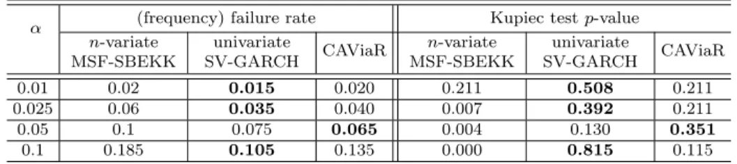
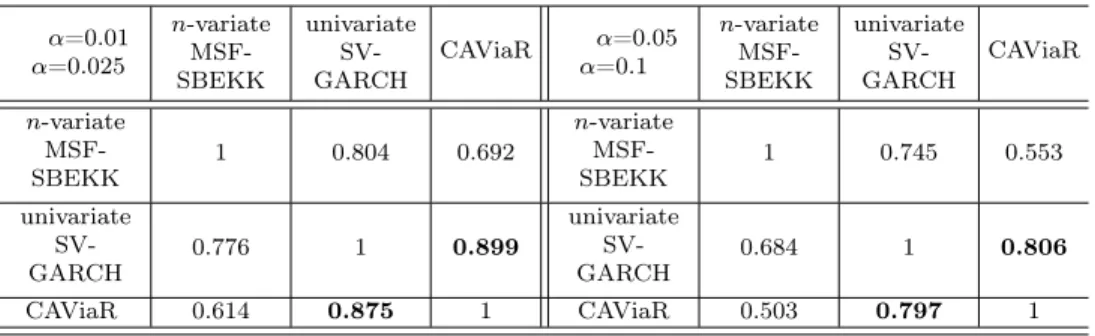
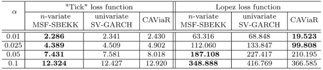
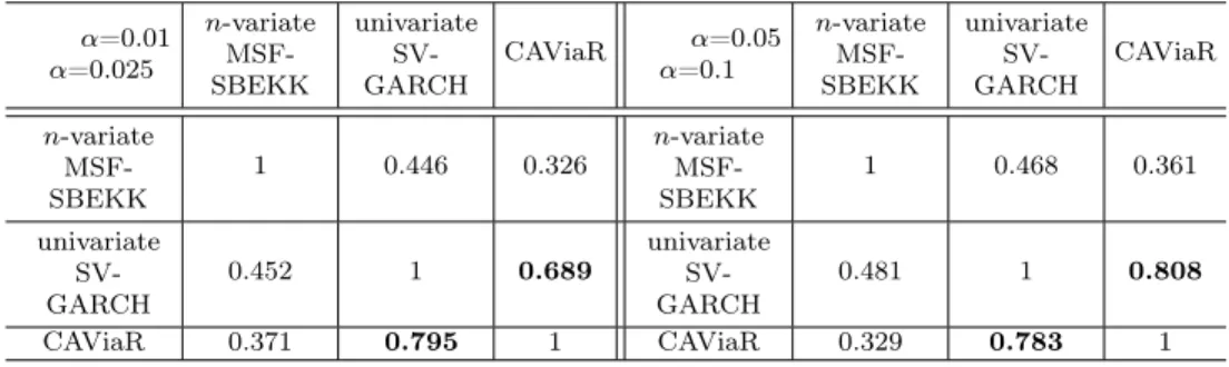
The outcomes of the Kupiec test for the 1-day ahead VaR seem to indicate that the univariate approach is more accurate and our Bayesian assessment competes with the one based on CAViaR (Table 2; the best case is in bold). The "tick" loss function does not give such a clear picture, but the Lopez and firms’ losses are smallest for our Bayesian VaR based on the univariate approach (Table 3 and 4). The results show that, in the case of this particular portfolio, then-variate MSF-SBEKK approach is unnecessary for risk assessment. On the other hand, the univariate special case gives us the flexible parametric SV-GARCH(1,1) specification that can be very successful in VaR analysis. It is usually not worse than CAViaR (sometimes much better) and leads to assessments that are highly correlated with the ones based on CAViaR; see Table 5.

In Tables 6 and 7 we present V aRt:t+s(α) results for all forecast horizons

(s= 1,2, . . . ,10); the results were obtained using univariate and n-variate

MSF-SBEKK models, respectively. The univariate SV-GARCH model gives better VaR forecasts for alls.

It may be the case that the approximate character of our posterior and predictive analysis, based on the OLS estimates of matrix parameters, is partly responsible for the poor performance of ourn-variate model. However, this is impossible to verify as the exact posterior analysis is infeasible for n= 34.

(12)

Table 2: The failure rate andp-value for the Kupiec test forV aRt:t+1(α), n= 34 α (frequency) failure rate Kupiec testp-value

n-variate MSF-SBEKK univariate SV-GARCH CAViaR n-variate MSF-SBEKK univariate SV-GARCH CAViaR 0.01 0.02 0.015 0.020 0.211 0.508 0.211 0.025 0.06 0.035 0.040 0.007 0.392 0.211 0.05 0.1 0.075 0.065 0.004 0.130 0.351 0.1 0.185 0.105 0.135 0.000 0.815 0.115

Note: The failure rate is defined as the proportion ofDt:t+1’s smaller than the−V aRt:t+1(α)

Table 3: "Tick" and Lopez loss functions forV aRt:t+1(α),n= 34 α "Tick" loss function Lopez loss function

Table 4: Firm’s loss functions forV aRt:t+1(α)and average loss on the portfolio when the loss is larger thanV aRt:t+1(α),n= 34

α

Firm’s loss function

withc= 0.000167(average WIBOR O/N rate)

Average loss on the portfolio when the loss is larger thanV aRt:t+1(α)

n-variate MSF-SBEKK univariate SV-GARCH CAViaR n-variate MSF-SBEKK univariate SV-GARCH CAViaR 0.01 19.178 17.979 29.947 170.848 168.680 170.848 0.025 85.052 64.076 81.025 133.508 149.227 136.856 0.05 221.522 145.575 181.894 119.272 129.937 115.975 0.1 509.010 324.577 361.007 93.605 118.261 100.464 J. Osiewalski, A. Pajor 264

(13)

Table 5: Correlation coefficients between V aRt:t+1(α) for α = 0.01 and α = 0.05 (upper part), forα= 0.025 andα= 0.1(lower part), n= 34

α=0.01 α=0.025 n-variate MSF-SBEKK univariate SV-GARCH CAViaR α=0.05 α=0.1 n-variate MSF-SBEKK univariate SV-GARCH CAViaR n-variate MSF-SBEKK 1 0.804 0.692 n-variate MSF-SBEKK 1 0.745 0.553 univariate SV-GARCH 0.776 1 0.899 univariate SV-GARCH 0.684 1 0.806 CAViaR 0.614 0.875 1 CAViaR 0.503 0.797 1

Table 6: V aRt:t+s(0.05)- univariate MSF-SBEKK (SV-GARCH),n= 34

s 1 2 3 4 5 6 7 8 9 10 FR 0.075 0.075 0.08 0.095 0.09 0.08 0.08 0.075 0.08 0.1 p-value for Kupiec test 0.1296 0.1296 0.0722 0.009 0.019 0.0722 0.0722 0.1296 0.0722 0.004 ALs 129.94 205.72 223.99 234.91 269.29 309.95 352.62 372.33 428.43 433.15 tick loss 7.6035 11.864 14.104 15.477 17.8 19.625 21.411 23.41 26.408 28.184 Lopez loss 1.3567 1.4166 1.3658 1.2836 1.3085 1.3539 1.3495 1.3872 1.4219 1.3519

Table 7: V aRt:t+s(0.05)–n-variate MSF-SBEKK,n= 34

s 1 2 3 4 5 6 7 8 9 10 FR 0.1 0.09 0.115 0.135 0.135 0.135 0.13 0.14 0.12 0.135 p-value for Kupiec test 0.004 0.019 0.0003 4·10 −6 ₄_·₁₀−6 ₄_·₁₀−6 ₁₀−6 ₁₀−6 _0.0001 ₄_·₁₀−6 ALs 119.27 194.72 202.63 220.73 245.24 281.7 313.44 325.8 388.05 398.16 tick loss 8.0514 13.438 15.295 17.546 19.886 22.623 25.379 27.841 31.546 35.001 Lopez loss 221.61 748.03 843.22 872.75 1266.7 1775.7 2280.1 3107.9 3891.2 4352.6 265 J. Osiewalski, A. Pajor CEJEME 2: 253-277 (2010)

(14)

6 VaR for a portfolio with 50 assets

6.1 One unit of each asset

Now we use stock data (on 50 companies) from the period May 13, 2005 – February, 23, 2010 (T = 1149); in February or March 2010 companies number 1–34 were included in mWIG40 and 35–50 in WIG20. Summary statistics for the daily percentage logarithmic returns (100rt,i) are shown in Table A2 in Appendix. Again, the

considered portfolio consists of one unit of each asset. The percentage logarithmic returns and daily changes of the portfolio value are shown in Figures 5 and 6, respectively. While the previous time series (of the same length) ended just before the financial crisis, now we analyse the data that include the whole period of market turbulences. So there are two new aspects: the financial crisis and a larger portfolio (n= 50). For then-variate model we use the same approximate Bayesian approach as previously. Again, we start withT = 998initial observations (now from the period May 13, 2005 – May, 12, 2009) and considerp= 200VaR assessments for 1-, 2- ,. . ., 10-day trading horizons. Note that our analysis covers the period of a slow recovery from the very deep crisis.

Figure 5: Daily growth rates of the portfolio value; n = 50 and a = (1, . . . ,1)0 (May 16, 2005 – February 23, 2010); the vertical line represents May 12, 2009

Figure 5. Daily growth rates of the portfolio with n=50 and a=(1, …, 1) (May 16, 2005 – February 23, 2010); the vertical line represents May 12, 2009

-8 -6 -4 -2 0 2 4 6 8 20 05 -05-1 6 20 05 -08-0 5 20 05 -10-2 7 20 06 -01-2 0 20 06 -04-1 2 20 06 -07-1 0 20 06 -09-2 9 20 06 -12-2 1 20 07 -03-1 6 20 07 -06-1 3 20 07 -09-0 4 20 07 -11-2 6 20 08 -02-2 1 20 08 -05-1 9 20 08 -08-0 8 20 08 -10-3 0 20 09 -01-2 8 20 09 -04-2 2 20 09 -07-1 5 20 09 -10-0 5 20 09 -12-2 9

Figure 6. Daily changes in the portfolio value (May 16, 2005 – February 23, 2010; n=50;

a=(1, …, 1)); the vertical line represents May 12, 2009

-500 -400 -300 -200 -100 0 100 200 300 400 500 2005 -0 5-16 2005 -0 8-05 2005 -1 0-27 2006 -0 1-20 2006 -0 4-12 2006 -0 7-10 2006 -0 9-29 2006 -1 2-21 2007 -0 3-16 2007 -0 6-13 2007 -0 9-04 2007 -1 1-26 2008 -0 2-21 2008 -0 5-19 2008 -0 8-08 2008 -1 0-30 2009 -0 1-28 2009 -0 4-22 2009 -0 7-15 2009 -1 0-05 2009 -1 2-29

The results presented for one day ahead VaR (Tables 8-10) clearly indicate that now then-variate approach is more accurate and that our Bayesian assessment (based on the parametric MSF-SBEKK structure) competes with the one based on CAViaR. Interestingly, VaRs based on univariate approaches (CAViaR and SV-GARCH) are highly correlated, as in the previous example; see Table 11. For this dataset the s -day ahead VaR for s > 1, obtained within the n-variate model, is worse (than the assessment based on the univariate SV-GARCH model) only with respect to the tick

J. Osiewalski, A. Pajor CEJEME 2: 253-277 (2010)

(15)

Bayesian Value-at-Risk for a Portfolio...

Figure 6: Daily changes in the portfolio value (May 16, 2005 – February 23, 2010;

n= 50;a= (1, . . . ,1)0); the vertical line represents May 12, 2009

30 February 23, 2010); the vertical line represents May 12, 2009

-8 -6 -4 -2 0 2 4 6 8 20 05 -05-1 6 20 05 -08-0 5 20 05 -10-2 7 20 06 -01-2 0 20 06 -04-1 2 20 06 -07-1 0 20 06 -09-2 9 20 06 -12-2 1 20 07 -03-1 6 20 07 -06-1 3 20 07 -09-0 4 20 07 -11-2 6 20 08 -02-2 1 20 08 -05-1 9 20 08 -08-0 8 20 08 -10-3 0 20 09 -01-2 8 20 09 -04-2 2 20 09 -07-1 5 20 09 -10-0 5 20 09 -12-2 9

a=(1, …, 1)); the vertical line represents May 12, 2009

-500 -400 -300 -200 -100 0 100 200 300 400 500 2005 -0 5-16 2005 -0 8-05 2005 -1 0-27 2006 -0 1-20 2006 -0 4-12 2006 -0 7-10 2006 -0 9-29 2006 -1 2-21 2007 -0 3-16 2007 -0 6-13 2007 -0 9-04 2007 -1 1-26 2008 -0 2-21 2008 -0 5-19 2008 -0 8-08 2008 -1 0-30 2009 -0 1-28 2009 -0 4-22 2009 -0 7-15 2009 -1 0-05 2009 -1 2-29

loss; it is usually much better in terms of the failure rate and Lopez loss (see Tables 12 and 13).

Table 8: The failure rate and p-value for the Kupiec test for V aRt:t+1(α), n = 50,

a= (1, . . . ,1)0

α (frequency) failure rate Kupiec testp-value n-variate MSF-SBEKK univariate SV-GARCH CAViaR n-variate MSF-SBEKK univariate SV-GARCH CAViaR 0.01 0.010 0.015 0.015 1.000 0.508 0.508 0.025 0.020 0.025 0.03 0.639 1.000 0.660 0.05 0.045 0.065 0.06 0.742 0.351 0.529 0.1 0.110 0.12 0.105 0.642 0.359 0.815

Table 9: "Tick" and Lopez loss functions forV aRt:t+1(α),n= 50,a= (1, . . . ,1)0

α "Tick" loss function Lopez loss function n-variate MSF-SBEKK univariate SV-GARCH CAViaR n-variate MSF-SBEKK univariate SV-GARCH CAViaR 0.01 2.286 2.341 2.430 63.316 68.848 19.523 0.025 4.389 4.509 4.902 112.060 133.847 99.808 0.05 7.431 7.581 8.018 187.108 227.417 210.195 0.1 12.324 12.427 12.920 348.888 416.769 366.585 267 J. Osiewalski, A. Pajor CEJEME 2: 253-277 (2010)

(16)

Table 10: Firm’s loss functions forV aRt:t+1(α)and average loss on the portfolio when the loss is larger thanV aRt:t+1(α),n= 50anda= (1, . . . ,1)0

α

n-variate MSF-SBEKK univariate SV-GARCH CAViaR n-variate MSF-SBEKK univariate SV-GARCH CAViaR 0.01 63.325 68.850 19.529 213.700 188.880 215.610 0.025 112.055 133.835 99.793 177.075 169.632 159.928 0.05 187.074 227.361 210.146 146.729 133.258 135.460 0.1 348.786 416.656 366.488 109.687 110.548 112.785 Figure 7: −V aRt:t+1(0.05)forn= 50,a= (1, . . . ,1)0 31 Figure 7. -VaRt:t+1 (0.05) for n=50, a=(1, …, 1)

-400 -300 -200 -100 0 100 200 2 009- 05-13 2 009- 06-01 2 009- 06-19 2 009- 07-08 2 009- 07-27 2 009- 08-13 2 0 09-01 2 0 09-18 2 009- 10-07 2 009- 10-26 2 009- 11-13 2 009- 12-02 2 009- 12-21 2 010- 01-12 2 010- 01-29 2 010- 02-17 D(t:t+1) univ. SV-GARCH n-variate MSF-SBEKK CAViaR

Figure 8. -VaRt:t+1 (0.01) for n=50, a=(1, …, 1)

-400 -300 -200 -100 0 100 200 200 9-0 5 -1 3 200 9-0 6 -0 1 200 9-0 6 -1 9 200 9-0 7 -0 8 200 9-0 7 -2 7 200 9-0 8 -1 3 200 9-0 9 -0 1 200 9-0 9 -1 8 200 9-1 0 -0 7 200 9-1 0 -2 6 200 9-1 1 -1 3 200 9-1 2 -0 2 200 9-1 2 -2 1 201 0-0 1 -1 2 201 0-0 1 -2 9 201 0-0 2 -1 7 D(t:t+1) univ. SV-GARCH n-variate MSF-SBEKK CAViaR

Table 11: Correlation coefficients between V aRt:t+1(α) for α= 0.01 and α = 0.05

(upper part), forα= 0.025andα= 0.1(lower part),n= 50,a= (1, . . . ,1)0

α=0.01 α=0.025 n-variate MSF-SBEKK univariate SV-GARCH CAViaR α=0.05 α=0.1 n-variate MSF-SBEKK univariate SV-GARCH CAViaR n-variate MSF-SBEKK 1 0.446 0.326 n-variate MSF-SBEKK 1 0.468 0.361 univariate SV-GARCH 0.452 1 0.689 univariate SV-GARCH 0.481 1 0.808 CAViaR 0.371 0.795 1 CAViaR 0.329 0.783 1 J. Osiewalski, A. Pajor 268

(17)

Bayesian Value-at-Risk for a Portfolio... Figure 8: −V aRt:t+1(0.01)forn= 50, a= (1, . . . ,1)0 31 -400 -300 -200 -100 0 100 200 2 009- 05-13 2 009- 06-01 2 009- 06-19 2 009- 07-08 2 009- 07-27 2 009- 08-13 2 0 09-01 2 0 09-18 2 009- 10-07 2 009- 10-26 2 009- 11-13 2 009- 12-02 2 009- 12-21 2 010- 01-12 2 010- 01-29 2 010- 02-17 D(t:t+1) univ. SV-GARCH n-variate MSF-SBEKK CAViaR

Figure 8. -VaRt:t+1 (0.01) for n=50, a=(1, …, 1)

-400 -300 -200 -100 0 100 200 200 9-0 5 -1 3 200 9-0 6 -0 1 200 9-0 6 -1 9 200 9-0 7 -0 8 200 9-0 7 -2 7 200 9-0 8 -1 3 200 9-0 9 -0 1 200 9-0 9 -1 8 200 9-1 0 -0 7 200 9-1 0 -2 6 200 9-1 1 -1 3 200 9-1 2 -0 2 200 9-1 2 -2 1 201 0-0 1 -1 2 201 0-0 1 -2 9 201 0-0 2 -1 7 D(t:t+1) univ. SV-GARCH n-variate MSF-SBEKK CAViaR

Table 12: V aRt:t+s(0.05) - univariate MSF-SBEKK (SV-GARCH), n = 50,

a= (1, . . . ,1)0 s 1 2 3 4 5 6 7 8 9 10 FR 0.1 0.075 0.07 0.085 0.065 0.075 0.09 0.07 0.065 0.085 p-value for Kupiec test 0.00 0.13 0.22 0.04 0.35 0.13 0.02 0.22 0.35 0.04 ALs 12.73 14.67 18.77 24.83 22.70 29.35 35.88 31.31 30.64 40.81 tick loss 7.57 9.99 12.88 14.64 17.16 19.49 19.56 21.37 22.94 24.07 Lopez loss 145.08 206.46 416.52 538.06 752.14 957.59 690.62 859.62 1140.31 1018.98

Table 13: V aRt:t+s(0.05)–n-variate MSF-SBEKK,n= 50,a= (1, . . . ,1)0

6.2 Comparable shares of assets

Now we use the same stock data as previously, but the considered portfolio consists of ai=aτ,i = 1 n n P i=1 Sτ,i

Sτ,i units of asseti, that is ωτ,i= 1

50, wherei= 1, . . . ,50, andτ represents May 12, 2009. (The values ofai are presented in the last column of Table

(18)

A2.) Of course, the sharesωτ,i vary over time, but they are more balanced than in

the previous case (with one unit of each asset). The logarithmic returns and daily changes of the portfolio value are shown in Figures 9 and 10, respectively. Again, we start withT = 998initial observations (from the period May 13, 2005 – May, 12, 2009) and considerp= 200VaR assessments for 1-,2-,. . ., 10-day trading horizons. The results for 1-day ahead VaR (Tables 14–16) do not lead to simple conclusions. Again, the univariate SV-GARCH model gives VAR assessments that are highly correlated with the ones based on CAViaR (Table 17). Which model is better depends on the particular criterion. For example, the "tick" loss indicates some preference for the n-variate MSF-SBEKK model, while the Lopez and firm’s loss suggest that CAViaR is the optimal model.

Figure 9: Daily growth rates of the portfolio value; n= 50 and ωτ,i = ₅₀1 (May 16,

2005 – February 23, 2010); the vertical line represents May 12, 2009 Figure 9. Daily growth rates of the portfolio with n=50 and ,i=1/50 (May 16, 2005 –

February 23, 2010); the vertical line represents May 12, 2009

-8 -6 -4 -2 0 2 4 6 8 20 05-0 5 -1 6 20 05-0 8 -0 5 20 05-1 0 -2 7 20 06-0 1 -2 0 20 06-0 4 -1 2 20 06-0 7 -1 0 20 06-0 9 -2 9 20 06-1 2 -2 1 20 07-0 3 -1 6 20 07-0 6 -1 3 20 07-0 9 -0 4 20 07-1 1 -2 6 20 08-0 2 -2 1 20 08-0 5 -1 9 20 08-0 8 -0 8 20 08-1 0 -3 0 20 09-0 1 -2 8 20 09-0 4 -2 2 20 09-0 7 -1 5 20 09-1 0 -0 5 20 09-1 2 -2 9

Figure 10. Daily changes in the portfolio value (May 16, 2005 – February 23, 2010; n=50; ,i=1/50); the vertical line represents May 12, 2009

-500 -400 -300 -200 -100 0 100 200 300 400 500 20 05-0 5 -1 6 20 05-0 8 -0 5 20 05-1 0 -2 7 20 06-0 1 -2 0 20 06-0 4 -1 2 20 06-0 7 -1 0 20 06-0 9 -2 9 20 06-1 2 -2 1 20 07-0 3 -1 6 20 07-0 6 -1 3 20 07-0 9 -0 4 20 07-1 1 -2 6 20 08-0 2 -2 1 20 08-0 5 -1 9 20 08-0 8 -0 8 20 08-1 0 -3 0 20 09-0 1 -2 8 20 09-0 4 -2 2 20 09-0 7 -1 5 20 09-1 0 -0 5 20 09-1 2 -2 9

Figure 10: Daily changes in the portfolio value (May 16, 2005 – February 23, 2010;

n= 50;ωτ,i= ₅₀1); the vertical line represents May 12, 2009

32 Figure 9. Daily growth rates of the portfolio with n=50 and ,i=1/50 (May 16, 2005 –

February 23, 2010); the vertical line represents May 12, 2009

-8 -6 -4 -2 0 2 4 6 8 20 05-0 5 -1 6 20 05-0 8 -0 5 20 05-1 0 -2 7 20 06-0 1 -2 0 20 06-0 4 -1 2 20 06-0 7 -1 0 20 06-0 9 -2 9 20 06-1 2 -2 1 20 07-0 3 -1 6 20 07-0 6 -1 3 20 07-0 9 -0 4 20 07-1 1 -2 6 20 08-0 2 -2 1 20 08-0 5 -1 9 20 08-0 8 -0 8 20 08-1 0 -3 0 20 09-0 1 -2 8 20 09-0 4 -2 2 20 09-0 7 -1 5 20 09-1 0 -0 5 20 09-1 2 -2 9

,i=1/50); the vertical line represents May 12, 2009

-500 -400 -300 -200 -100 0 100 200 300 400 500 20 05-0 5 -1 6 20 05-0 8 -0 5 20 05-1 0 -2 7 20 06-0 1 -2 0 20 06-0 4 -1 2 20 06-0 7 -1 0 20 06-0 9 -2 9 20 06-1 2 -2 1 20 07-0 3 -1 6 20 07-0 6 -1 3 20 07-0 9 -0 4 20 07-1 1 -2 6 20 08-0 2 -2 1 20 08-0 5 -1 9 20 08-0 8 -0 8 20 08-1 0 -3 0 20 09-0 1 -2 8 20 09-0 4 -2 2 20 09-0 7 -1 5 20 09-1 0 -0 5 20 09-1 2 -2 9 J. Osiewalski, A. Pajor CEJEME 2: 253-277 (2010) 270

(19)

As previously, we also consider thes-day ahead VaR fors >1. Again, according to the Lopez loss criterion, the n-variate MSF-SBEKK model is better than its univariate counterpart (the SV-GARCH model); the latter becomes important if we focus on the tick loss fors >6 and Kupiec test fors >2 (see Tables 18 and 19).

Note that the empirical findings obtained for the porftolio with balanced shares are not very similar to the previous ones, based on the portfolio with one unit of each asset. And both are different from the outcomes for the porfolio in Section 5 (n= 34), so any generalisation of our empirical results is hardly possible.

Finally, in Table 20 we present the posterior means and standard deviations, based on the whole time series, for basic MSF-SBEKK parameters (given the OLS estimates of the remaining parameters); we also show the results for the previous dataset (n= 34). The approximate posterior moments in n-variate models are very similar for the two datasets, but their counterparts in univariate SV-GARCH models are different between the datasets and portfolios (and from then-variate cases) and show that the SV part is crucial.

Table 14: The failure rate andp-value for the Kupiec test for V aRt:t+1(α),n= 50,

ωτ,i= ₅₀1

α (frequency) failure rate Kupiec testp-value n-variate MSF-SBEKK univariate SV-GARCH CAViaR n-variate MSF-SBEKK univariate SV-GARCH CAViaR 0.01 0.01 0.02 0.01 1.000 0.211 1.000 0.025 0.02 0.025 0.025 0.639 1.000 1.000 0.05 0.055 0.04 0.035 0.749 0.502 0.305 0.1 0.09 0.1 0.09 0.632 1.000 0.632

Table 15: "Tick" and Lopez loss functions forV aRt:t+1(α),n= 50andωτ,i= ₅₀1 α "Tick" loss function Lopez loss function

n-variate MSF-SBEKK univariate SV-GARCH CAViaR n-variate MSF-SBEKK univariate SV-GARCH CAViaR 0.01 1.991 2.084 1.971 20.691 18.022 6.400 0.025 3.942 4.258 4.210 52.341 71.158 13.531 0.05 6.729 6.894 7.211 106.337 146.965 85.306 0.1 11.139 10.996 11.464 241.865 284.189 228.027 271 J. Osiewalski, A. Pajor CEJEME 2: 253-277 (2010)

(20)

Table 16: Firm’s loss functions forV aRt:t+1(α)and average loss on the portfolio when the loss is larger thanV aRt:t+1(α),n= 50andωτ,i= ₅₀1

α

Figure 11: −V aRt:t+1(0.05)forn= 50,ωτ,i= 501 Figure 11. -VaRt:t+1 (0.05) for n=50 and ,i=1/50

-400 -300 -200 -100 0 100 200 200 9- 05-13 200 9- 06-01 200 9- 06-19 200 9- 07-08 200 9- 07-27 200 9- 08-13 200 9- 09-01 200 9- 09-18 200 9- 10-07 200 9- 10-26 200 9- 11-13 200 9- 12-02 200 9- 12-21 201 0- 01-12 201 0- 01-29 201 0- 02-17 D(t:t+1) univ. SV-GARCH n-variate MSF-SBEKK CAViaR

Figure 12. -VaRt:t+1 (0.01) for n=50 and ,i=1/50

-400 -300 -200 -100 0 100 200 2009- 05-13 2009- 06-01 2009- 06-19 2009- 07-08 2009- 07-27 2009- 08-13 20 09-01 20 09-18 2009- 10-07 2009- 10-26 2009- 11-13 2009- 12-02 2009- 12-21 2010- 01-12 2010- 01-29 2010- 02-17 D(t:t+1) univ. SV-GARCH n-variate MSF-SBEKK CAViaR Figure 12: −V aRt:t+1(0.01)forn= 50,ωτ,i= ₅₀1

33 Figure 11. -VaRt:t+1 (0.05) for n=50 and ,i=1/50

-400 -300 -200 -100 0 100 200 200 9- 05-13 200 9- 06-01 200 9- 06-19 200 9- 07-08 200 9- 07-27 200 9- 08-13 200 9- 09-01 200 9- 09-18 200 9- 10-07 200 9- 10-26 200 9- 11-13 200 9- 12-02 200 9- 12-21 201 0- 01-12 201 0- 01-29 201 0- 02-17 D(t:t+1) univ. SV-GARCH n-variate MSF-SBEKK CAViaR

Figure 12. -VaRt:t+1 (0.01) for n=50 and ,i=1/50

-400 -300 -200 -100 0 100 200 2009- 05-13 2009- 06-01 2009- 06-19 2009- 07-08 2009- 07-27 2009- 08-13 20 09-01 20 09-18 2009- 10-07 2009- 10-26 2009- 11-13 2009- 12-02 2009- 12-21 2010- 01-12 2010- 01-29 2010- 02-17 D(t:t+1) univ. SV-GARCH n-variate MSF-SBEKK CAViaR J. Osiewalski, A. Pajor CEJEME 2: 253-277 (2010) 272

(21)

Table 17: Correlation coefficients between V aRt:t+1(α) for α = 0.01 and α = 0.05 (upper part), forα= 0.025 andα= 0.1(lower part), n= 50, ωτ,i=₅₀1

α=0.01 α=0.025 n-variate MSF-SBEKK univariate SV-GARCH CAViaR α=0.05 α=0.1 n-variate MSF-SBEKK univariate SV-GARCH CAViaR n-variate MSF-SBEKK 1 0.362 0.264 n-variate MSF-SBEKK 1 0.372 0.247 univariate SV-GARCH 0.355 1 0.902 univariate SV-GARCH 0.402 1 0.986 CAViaR 0.276 0.847 1 CAViaR 0.247 0.765 1

Table 18: V aRt:t+s(0.05)- univariate MSF-SBEKK (SV-GARCH),n= 50,ωτ,i=501

Table 19: V aRt:t+s(0.05)– n-variate MSF-SBEKK,n= 50,ωτ,i= ₅₀1

s 1 2 3 4 5 6 7 8 9 10 FR 0.040 0.030 0.040 0.040 0.045 0.040 0.035 0.005 0.010 0.005 p-value for Kupiec test 0.749 0.502 0.305 0.074 0.008 0.002 0.008 0.000 0.000 0.000 ALs 122.42 182.49 229.79 269.80 277.70 345.78 350.23 353.36 0 0 tick loss 6.729 10.503 12.372 13.375 14.266 16.457 17.801 18.506 19.708 20.962 Lopez loss 106.34 329.20 258.96 70.42 4.87 108.37 42.37 1.54 0.00 0.00

7 Concluding remarks

The aim of the paper was threefold. First, we wanted to compare the n-variate and univariate approaches to risk assessment for a large portfolio. Second, we were eager to learn how the new hybrid MSF-SBEKK type I specification would work in

(22)

Table 20: Posterior means (and standard deviations) of the main MSF-SBEKK parameters Example model φ σ2 g β γ β+γ n= 34 T = 1149 n-variate 0.4995 0.1874 0.0167 0.8523 0.8690 (0.0339) (0.0113) (0.0014) (0.0180) (0.0168) univariate a= (1, . . . ,1) 0.9817 0.0117 0.0145 0.3105 0.3253 (0.0100) (0.0057) (0.0120) (0.1970) (0.1965) n-variate 0.5658 0.1223 0.0119 0.8423 0.8542 (0.0311) (0.0076) (0.0010) (0.0184) (0.0177) n= 50 T = 1198 univariate a= (1, . . . ,1) 0.9576 0.0351 0.0178 0.6650 0.6828 (0.0334) (0.0196) (0.0159) (0.2927) (0.2869) univariate ωτ,i=₅₀1 0.9621 0.0479 0.0084 0.6331 0.6425 (0.0171) (0.0177) (0.0075) (0.2949) (0.2934)

practice. Third, we wanted to show the merits of the Bayesian parametric approach to Value-at-Risk.

It is not clear that, for VaR assessment, univariate modelling (of portfolio value – instead of portfolio components) is enough as we initially (wrongly) conjectured. Multivariate specifications of asset prices are necessary for portfolio choice or optimisation, and they may be useful for forecasting future returns on a given portfolio as well. Thus, the n-variate MSF-BEKK model may occur practical and useful also in VaR analysis for large portfolios.

Our empirical study shows that the new hybrid n-variate and univariate models behave quite well and can compete with the CAViaR nonparametric specification. They are important all-purpose alternatives to non-parametric models that were designed to focus on specific aspects of future returns (and not on their full predictive distribution). Note that our univariate hybrid model appears as an interesting by-product of the multivariate analysis. It is a new parametric model that integrates flexibility of the basic SV structure and simplicity of the GARCH(1,1) specification. However, our results suggest that the GARCH part may be unnecessary when the posterior distribution of its parameters is not sharp enough as to exclude zero values. A formal comparison between the pure SV and hybrid SV-GARCH(1,1) models would require calculating the Bayes factor, which is beyond the scope of this paper. Finally, the paper indicates that the Bayesian approach to VaR analysis is fully relevant and practical. Remind that conditioning on observed data as well as inference on non-linear functions of unobserved quantities (future logarithmic returns) are necessary for any appropriate VaR analysis. Both are natural and easy within Bayesian statistics, equipped with the Markov Chain Monte Carlo (MCMC) simulation tools.

(23)

Acknowledgements

The authors would like to thank an anonymous referee for very important comments on manuscript, and Łukasz Kwiatkowski for careful reading of the first version and useful suggestions.

References

[1] Artzner P., Delbaen F., Eber J.-M., Heath D., (1999), Coherent measures of risk, Mathematical Finance 9, 203-228.

[2] Bauwens L., Laurent S., Rombouts J.V.K., (2006), Multivariate GARCH models: A survey,Journal of Applied Econometrics 21, 79-109.

[3] Engle R., Manganelli S., (2004), CAViaR: conditional autoregressive Value at Risk by regression quantiles, Journal of Business and Economic Statistics 22, 367-381.

[4] Lee T. H., (2008), Loss Functions in Time Series Forecasting, [in:] International Encyclopedia of the Social Sciences, 2nd _{edition. Vol. 4, Macmillan Reference}

USA, Detroit.

[5] Lopez J.A., (1998), Testing your risk tests, The Financial Survey, May–June, 18-20.

[6] O’Hagan A., (1994),Bayesian Inference, Edward Arnold, London.

[7] Osiewalski J., (2009), New hybrid models of multivariate volatility (a Bayesian perspective),Przegląd Statystyczny (Statistical Review) 56, 15-22.

[8] Osiewalski J., Pajor A., (2009), Bayesian analysis for hybrid MSF-SBEKK models of multivariate volatility, Central European Journal of Economic Modelling and Econometrics 1, 179-202.

[9] Pajor A., (2005), Bayesian comparison of bivariate SV models for two related time series,Acta Universitatis Lodziensis – Folia Oeconomica 190, 177-196. [10] Sarma M., Thomas S., Shah A., (2003), Selection of Value-at-Risk Models,

Journal of Forecasting 22, 337-358.

[11] Tsay R.S., (2005), Analysis of Financial Time Series (2nd _{edition), Wiley, New}

York.

(24)

Appendix

Table A1: Sample characteristics for the first dataset (January 30, 2003 – August 29, 2007;n= 34)

Number company average variance kurtosis minimum maximum 1 BPH 0.111 3.633 5.566 -10.566 9.444 2 BDX 0.099 5.738 10.848 -10.807 21.035 3 DUD 0.142 7.464 84.896 -47.505 12.936 4 ECH 0.205 3.570 6.588 -8.278 8.961 5 EMP 0.207 6.703 74.053 -15.575 43.621 6 GRJ 0.187 4.741 10.388 -12.516 15.453 7 BHW 0.054 2.506 28.503 -20.096 8.734 8 BSK 0.096 1.883 7.090 -6.432 6.652 9 KTY 0.112 3.760 5.918 -11.823 9.019 10 KPX 0.318 11.768 19.581 -15.082 35.398 11 KRB 0.048 3.423 20.872 -21.472 8.961 12 MCI 0.370 13.946 11.538 -20.373 33.178 13 MIL 0.130 5.004 9.131 -12.783 14.458 14 MSX 0.160 13.792 12.555 -24.381 28.768 15 MSZ 0.227 18.058 8.234 -25.300 23.974 16 NET 0.021 3.757 16.142 -20.567 8.444 17 EMF 0.093 9.001 15.841 -22.012 24.686 18 ORB 0.126 4.192 7.993 -15.558 10.178 19 PGF 0.101 4.327 16.119 -10.536 21.767 20 PRC 0.027 24.506 11.560 -28.768 34.484 21 STX 0.099 14.130 12.677 -29.523 23.863 22 STP 0.395 7.523 11.815 -9.237 23.309 23 VST 0.325 7.615 9.840 -10.536 18.666 24 AGO 0.007 4.281 5.500 -11.955 8.072 25 BRE 0.167 3.594 5.007 -7.633 8.898 26 BZW 0.109 4.270 4.090 -8.259 7.496 27 CST 0.193 3.802 9.514 -10.488 13.262 28 GTN 0.208 11.946 35.008 -45.392 24.613 29 KGH 0.182 6.471 5.679 -15.590 9.093 30 PEO 0.086 3.854 4.759 -6.579 11.919 31 PKN 0.100 3.610 3.893 -9.298 7.746 32 PXM 0.349 7.723 7.441 -11.725 16.252 33 PND 0.247 16.735 34.983 -53.870 28.395 34 TPS 0.045 3.237 3.731 -8.359 5.617 J. Osiewalski, A. Pajor 276

(25)

Table A2: Sample characteristics for the first dataset (May 13, 2005 – February 23, 2010,n= 50)

Number company average variance kurtosis minimum maximum ai

1 HANDLOWY 0.007 4.854 11.292 -20.096 9.225 1.413 2 INGBSK 0.037 4.897 6.856 -11.647 9.531 0.244 3 NETIA 0.016 3.792 6.764 -10.110 9.531 21.339 4 LPP 0.072 6.020 7.223 -12.234 17.300 0.073 5 STALPROD 0.164 7.635 5.399 -10.882 14.618 0.163 6 SWIECIE 0.033 4.885 6.807 -11.123 12.925 1.560 7 MILLENNIUM 0.026 9.748 6.466 -16.190 14.458 29.605 8 EMPERIA 0.068 7.473 59.876 -18.232 43.621 1.528 9 EUROCASH 0.129 6.005 5.349 -8.224 12.260 6.872 10 KETY 0.002 5.228 6.380 -12.604 12.047 0.992 11 AMREST 0.094 6.069 6.126 -10.821 11.588 1.466 12 ECHO 0.049 8.247 5.948 -11.778 15.498 24.006 13 CCC 0.109 5.618 5.211 -11.584 9.858 1.925 14 BUDIMEX 0.043 6.849 8.383 -10.807 21.035 1.019 15 ELBUDOWA 0.165 5.547 5.456 -8.895 14.041 0.499 16 ORBIS 0.030 6.583 7.285 -15.558 14.497 1.683 17 SYGNITY -0.165 9.074 8.915 -19.776 21.481 3.608 18 MOSTALWAR 0.209 7.146 6.704 -14.559 16.380 1.353 19 KOGENERA 0.096 5.282 10.381 -13.976 18.623 1.049 20 PEP 0.131 6.179 10.309 -19.980 14.914 2.619 21 NFIEMF 0.079 10.747 10.251 -18.447 24.686 6.821 22 MCI 0.072 15.610 10.049 -20.373 33.178 15.936 23 CIECH 0.020 6.529 9.109 -17.313 13.604 2.203 24 KOPEX 0.148 11.698 9.716 -15.763 28.174 4.014 25 POLNORD 0.105 18.393 27.961 -53.870 28.395 2.304 26 ALCHEMIA 0.126 11.403 15.487 -19.863 30.295 10.777 27 MOSTALZAB 0.151 14.937 6.727 -15.894 23.974 17.707 28 VISTULA -0.003 11.648 9.974 -24.512 18.232 58.976 29 GANT 0.215 29.602 15.746 -51.975 33.547 2.610 30 IMPEXMET 0.034 11.864 9.416 -14.542 25.131 45.394 31 STALEXP 0.003 13.214 9.945 -21.337 26.065 48.013 32 DUDA -0.182 15.286 33.898 -47.505 22.314 79.680 33 MOL 0.000 8.952 8.561 -18.232 17.869 0.408 34 KREDYTB 0.041 5.561 37.723 -33.024 13.414 11.703 35 AGORA -0.081 7.534 5.656 -16.919 10.851 4.746 36 PEKAO 0.019 8.040 6.733 -20.585 13.556 0.635 37 KGHM 0.098 11.039 7.336 -23.624 17.693 1.101 38 PKNORLEN -0.023 6.404 4.637 -12.158 12.866 2.675 39 PKOBP 0.026 6.176 4.736 -12.223 9.973 2.623 40 TPSA -0.014 4.092 3.964 -9.022 8.080 4.327 41 BZWBK 0.053 7.845 4.225 -12.143 11.030 0.776 42 ASSECOPOL 0.070 5.295 9.483 -19.506 13.384 1.443 43 GETIN 0.083 7.456 8.714 -14.957 19.479 12.825 44 GTC 0.055 9.773 5.939 -14.660 17.280 4.115 45 TVN 0.043 7.151 6.331 -15.932 12.859 6.840 46 BRE 0.054 8.092 6.212 -14.150 12.900 0.477 47 PBG 0.110 5.341 4.875 -10.003 9.278 0.360 48 POLIMEXMS 0.105 7.982 5.608 -11.725 14.537 19.973 49 CERSANIT 0.028 8.836 5.328 -13.453 13.573 5.467 50 BIOTON -0.037 14.935 6.687 -16.705 20.479 277.406 277 J. Osiewalski, A. Pajor CEJEME 2: 253-277 (2010)