Identification Robust Confidence Sets Methods for Inference on Parameter Ratios and their Application to Estimating Value-of-Time

(1)

Identification Robust Confidence Sets Methods for Inference on

Parameter Ratios and their Application to Estimating

Value-of-Time and Elasticities

Denis Bolduc

1

Université Laval

Lynda Khalaf

2

Université Laval

Clément Yélou

3

Université Laval

May 30, 2005

1_{Groupe de recherche en économie de l’énergie, de l’environnement et des ressources naturelles}

[GREEN], Université Laval. Mailing address: Pavillon J.-A.-De Sève, St. Foy, Québec, Canada, G1K 7P4. TEL: (418) 656-5427; FAX: (418) 656-2707; Email: [email protected].

[GREEN], Université Laval. Mailing address: Pavillon J.-A.-De Sève, St. Foy, Québec, Canada, G1K 7P4. TEL: (418) 656 2131-2409; FAX: (418) 656 7412; Email: [email protected].

[GREEN], Université Laval. Mailing address: Pavillon J.-A.-De Sève, St. Foy, Québec, Canada, G1K 7P4. Email: [email protected].

(2)

Abstract

The problem of constructing confidence set estimates for parameter ratios arises in a variety of econometrics contexts; these include value-of-time estimation in transportation research and inference on elasticities given several model specifications. Even when the model under consider-ation is identifiable, parameter ratios involve a possibly discontinuous parameter transformation that becomes ill-behaved as the denominator parameter approaches zero. More precisely, the parameter ratio is not identified over the whole parameter space: it is locally almost unidentified

or (equivalently) weakly identified over a subset of the parameter space. It is well known that

such situations can strongly aﬀect the distributions of estimators and test statistics, leading to the failure of standard asymptotic approximations, as shown by Dufour (1997). Here, we provide explicit solutions for projection-based simultaneous confidence sets for ratios of parameters when

the joint confidence set is obtained through a generalized Fieller approach. The procedures are

applied and compared in illustrative simulated and empirical examples, with a focus on choice models.

Key words: confidence set; generalized Fieller’s theorem; delta-method; Weak identifi ca-tion; parameter transformation.

(3)

List of Tables

1 Empirical coverage rates for the delta method- and the Fieller method- based confidence intervals for a parameter ratio in a simple binary probit model. . . 8

2 Empirical coverage rates for the delta method- and the Fieller method- based confidence intervals for a parameter ratio in a kernel logit multinomial probit model. . . 11

3 Simultaneous confidence sets for values of total travel time and of out-of-vehicle time from a trinomial logit model analyzed in Ben-Akiva and Lerman, 1985. . . . 19

4 Simultaneous confidence sets for values of time as percentage of net personal income. 20 5 Simultaneous confidence sets for values of time as percentage of net personal income. 21 6 Simultaneous confidence sets for long run price- and income- elasticities of total energy demand. . . 22

(4)

1 Introduction

The problem of constructing confidence set estimates for parameter ratios arises in a variety

of econometrics contexts; these include value-of-time estimation in transportation research, or inference on elasticities in demand or cost analysis. Even when the model under consideration

is identifiable, parameter ratios involve a possibly discontinuous parameter transformation that

becomes ill-behaved as the denominator parameter approaches zero. More precisely, the para-meter ratio is not identified over the whole parameter space: it is locally almost unidentified

over a nonidentification subset of the parameter space. Important examples include inference

on elasticities (t-statistics and confidence intervals) in demand systems [Deaton and Muellbauer

(1980); Banks, Blundell and Lewbel (1997)], and inference onfixed value of time in discret choice

transportation models (Bolduc (1999)). It is well known that such situations can strongly aﬀect

the distributions of estimators and test statistics, leading to the failure of standard asymptotic approximations, as shown by Dufour (1997, 2003).

The delta-method, which is an asymptotically justified Wald-type method, provides a

com-mon procedure to construct Wald-type confidence sets (CI) for ratios of parameters or ratios of

linear combinations of parameters in econometric models. In the statistics literature, Fieller’s theorem [Fieller (1940, 1954)] gives a simple way to obtain an exact confidence interval (CI) for

the ratio of two means of normal variates. Scheﬀé (1970) proposes a modification of Fieller’s

procedure, which avoids trivial confidence set, i.e. confidence sets which cover the entire real

line.1 Zerbe, Laska, Meisner and Kushner (1982) extend Fieller’s theorem in two directions.

First, they focus on ratios of parameters in the normal linear regression model. Secondly, they construct multivariate confidence regions and simultaneous confidence sets for several ratios of linear combinations of parameters. In this case, normality still guarantees exact confidence lev-els. Young, Zerbe and Hay (1997) applies Zerbe et al. (1982)’s results to the context of linear and

nonlinear mixed-eﬀects models, in which case the distribution of estimators and test statistics

are asymptotic.

Athough the solution provided by Fieller’s method has been analyzed to some extent in the statistics litterature on location-scale, ANOVA and regression models [Darby (1980); Selwyn and Hall (1984); Buonaccorsi (1985); Bucephala and Gatsonis (1988); Zerbe (1978); Zerbe et al. (1982); Young et al. (1997)], its application to discret choice or limited dependent variable models is rather little documented. There is substantial evidence that standard asymptotics provides poor approximation to the sampling distribution of estimators and test statistics in discret choice or limited dependent variable models, even when linear hypothesis tests are of concern [see Davidson and MacKinnon (1999b), Davidson and MacKinnon (1999a), Davidson and MacKinnon (2000) and Savin and Würtz (1998)]. Furthermore, Dufour (1997) shows that most Wald-type confidence sets for a locally almost unidentified parameter in econometric models

where the parameter space contains a nonidentification subset deviate arbitrarily from their

nominal level, since they are almost surely bounded. In view of the recent literature on weak 1

Scheﬀé (1970)’s procedure proceeds as follows: first test the null hypothesis that the numerator and the

denominator are jointly equal to zero. If this test does not reject, state that both the numerator and the

denominator jointly take on zero value. If the test rejects, state that the ratio is inside or outside afinite modified

(5)

identification and weak instruments [Dufour (1997), Stock, Wright and Yogo (2002), Stock and Yogo (2002), Dufour (2003), Stock and Wright (2000)], there has been a renewed interest in an alternative method based on generalizing Fieller’s theorem [Fieller (1940, 1954)]. In this paper, we consider Fieller-type simultaneous confidence sets for multiple ratio functions in econometric models under (2.1)-(2.2) below, with a focus on discret choice models. Our contributions can be classified into three categories.

First, we provide evidence based on two simulation studies that the delta method based

confidence set for one parameter ratio in a discret choice model performs very poorly when the

denominator approaches zero. One simulation study is based on a simple binary probit model,

and the other one is based on a more complex model, a multinomial probit model withfirst-order

generalized autoregressive errors [Bolduc (1992, 1999)].

Second, we use projection techniques to derive explicit form for simultaneous confidence sets

for scalar linear transformations of afinite number of parameter ratios in general econometric

models. Our characterization result shows that the confidence sets are not necessarily bounded,

which implies that they will not suﬀer from the fundamental limitations documented in Dufour

(1997). Our results hold asymptotically under mild regularity conditions and exactly for special cases. This extends work by Zerbe et al. (1982) beyond the normal linear regression model.

Third, the proposed procedures are applied to the transportation behavior analysis using the

multinomial probit model specified and estimated in Bolduc (1999), where inference for three

value of time ratios was relies on t-statistics based on the delta method.

The paper is organized as follows. In section 2, we set notation and introduce the statistical

framework. In section 3, we discuss two methods for constructing a confidence interval for one

parameters ratio and examine their statistical performance in illustrative discrete choice models. In section 4, we construct a Fieller-type joint confidence set for a finite number of ratios and

then we derive projection-based simultaneous confidence sets. Empirical applications of the

procedures are presented in section 5. Section 6 concludes.

2 Statistical Framework

In this section, we set notation and introduce the statistical framework. Consider the general parametric model

(_Y,_{Pθ, θ∈Θ⊂Rp, p≥1}), (2.1)

where_Y is the observations set, Pθ is a probability distribution over Y and θ= (θ1, θ2, ..., θp)0

is the parameter vector. The model is regular and identifiable, so based on a sample of size T,

there exists a consistent and asymptotically normal estimator ˆθ= (ˆθ1,ˆθ2, ...,ˆθp)0ofθ: ³

ˆ θ₋θ

´

−→N¡0,Σˆ_θ¢, T _{→ ∞}, (2.2)

wheredet¡Σˆ_θ¢₆= 0. LetΣˆˆ_θ denote a consistent estimate ofΣˆ_θ. For any constinuously diﬀ eren-tiable functiong :Θ∗ _−→_Rq, (q _≥1), where Θ∗ _⊆Θ, ifˆθ _∈Θ∗, then g³ˆθ´ is asymptotically

(6)

normal with meang(θ) and estimated variance matrixΣˆ_g(ˆ_θ) given by ˆ Σ_g(ˆ_{θ) =} ∂g ³ ˆ θ ´ ∂θ0 ˆ Σˆ_θ ∂g0 ³ ˆ θ ´ ∂θ . (2.3)

As a special case, any linear combination L0ˆθ of the elements of ˆθ, where L is a known p×1 vector, is asymptotically normal with estimated variance

ˆ

Σ_L₀ˆ_θ =L0Σˆˆ_θL. (2.4)

We consider Fieller-type confidence sets for ratio functions in econometric models under

(2.1)-(2.2), with a focus on discret choice models. We first examine, through illustrative empirical

models and Monte Carlo simulation studies, the poor performance of the delta method-based

confidence set for one parameter ratio. The latter confidence set is a Wald-type method based

on (2.3). Then, we consider the problem ofsimultaneous confidence sets for multiple ratios, in

which case we propose to use a theory of quadric confidence sets in order to derive the explicit

form of the simultaneous confidence limits for any scalar linear combination of these ratios.

So, our purpose is to build simultaneous confidence sets for scalar linear transformations of

the components of vector-valued ratio functionsh:Θ_−→_Rq, h(θ) = (h1(θ), h2(θ), ..., hq(θ))0.

Individual confidence sets for several parameters are said to be simultaneous if they are

con-structed ensuring an overall confidence level control; see Miller (1981), Dufour (1989),

Ab-delkhalek and Dufour (1998).

Definition 1 In the framework of model2.1-2.2, let_{gi(θ) :i∈I}be a set of parameters defined as functions of θ, where the index set I may be finite or infinite and gi(θ) ∈R,∀ i∈I and let CSi ⊂ R be a confidence set for gi(θ),∀ i ∈ I. The sets CSi, i ∈ I, constitute simultaneous confidence sets with level 1₋αfor gi(θ), i∈I if and only if

Pr (gi(θ)∈CSi, i∈I)≥1−α. (2.5)

A key feature of a ratio function, e.g. hi(θ), i= 1, ..., q,is that it may display discontinuities

in its domain Θ, so a reliable confidence set should be immune to such possible discontinuity

problems. Specifically, the coverage probability should be close to the nominal confidence level, even when the true value of the parameter vector is in a discontinuity boundary.

We consider the case where hi(θ) = L0_iθ/K0θ, where Li and K are known p×1 vectors, i = 1, ..., q. Ratios with the same denominator are encountered in many fields in economics; these include long run elasticities in dynamic demand models, and the economic value of time for several use-specific portions of travel time in transportation research. In this context, the discontinuity set for any hi, i= 1, ..., q, is the set of all θ ∈ Θ such that K0θ = 0. Our setup covers simultaneous confidence sets for the individual ratioshi(θ) or for linear combinations of hi(θ), i= 1, ..., q.For these cases, we apply projection techniques to a joint confidence region constructed for the vectorh(θ) = (h1(θ), ..., hq(θ))0.

(7)

3 Con

fi

dence Set for One Ratio of Parameters

In this section, we illustrate statistical problems associated with a confidence set constructed

for one parameter ratio using the delta method. For convenience, wefirst give a brief discussion

of two confidence set procedures, one based on the delta method and the other based on the

Fieller’s theorem, as they apply to the ratioδ(θ) =θ1/θ2 defined from model (2.1). Let ˆ Σ12= · ˆ v1 vˆ12 ˆ v12 vˆ2 ¸

denote the submatrix ofΣˆˆ_θ that corresponds to ³

ˆ_θ₁_,ˆ_θ₂´_.

3.1 The delta method and the Fieller-type con

fi

dence sets

The well-known delta-method relies on a first order Taylor series approximation for the

ra-tio funcra-tion δ(θ) = θ1/θ2 to obtain an estimate for the asymptotic variance of its maximum

likelihood estimatorˆδ = ˆθ1/ˆθ2. This estimated asymptotic variance is ˆ Σ_δ₍_βˆ_{) =}Gˆ0Σˆ12G,ˆ where ˆ G= " 1 ˆ θ2 , −ˆθ1 ˆ θ2₂ #₀ .

To get a(1₋α)level confidence set, the delta method yields the following Wald-type confidence set, using the asymptotic normal distribution critical pointz_α/2 :

DCS (δ; 1₋α) = " ˆ θ1 ˆ θ2 −zα/2Σˆ 1/2 δ(ˆ_θ), ˆ θ1 ˆ θ2 +zα/2Σˆ 1/2 δ(ˆ_θ) # . (3.6)

This confidence set is bounded and may therefore have zerocoverage probability. In other words,

the probability that this confidence set misses the true ratio may be practically one (Dufour

(1997)).

On the other hand, Fieller’ theorem, introduced in the context of the ratio of two means of normal variates where it leads to exact confidence sets, inverts a t-test of a linear restriction associated to the ratio. Inverting a test with respect to a parameter actually means that we

collect all the values of this parameter for which the test is not significant. For the ratio

δ(θ) =θ1/θ2 in the context of model (2.1)-2.2, it applies as follows. For each possible valueδ0 of the ratio, define the auxiliary hypothesis Hδ0:

Hδ0 : θ1−δ0θ2= 0. (3.7)

Then, a(1₋α)level confidence set corresponds to the set ofδ0 for which an t-test ofHδ0 is not

significant at levelα. The test statistic in question is defined by: t(δ0) = ³ ˆ θ1−δ0ˆθ2 ´ σ₍ˆ_θ₁₋_δ₀ˆ_θ₂₎ , (3.8)

(8)

where

σ₍ˆ_θ₁₋_δ₀ˆ_θ₂_{) =} ¡

δ2₀ˆv2−2δ0ˆv12+ ˆv1 ¢1/2 is an estimate of the variance of³ˆθ1−δ0ˆθ2

´

. UnderHδ0,

t(δ0)asy_∼ N (0,1).

So, Fieller’ theorem gives a(1₋α) level confidence set as the set of δ0 such that |t(δ0)_|_≤zα/2,

which leads to the following confidence set FCS (δ; 1₋α) = ½ δ0 : ³ ˆ θ1−δ0ˆθ2 ´2 ≤z_α/22 ¡vˆ1+δ02vˆ2−2δ0vˆ12 ¢¾ . (3.9)

This requires solving the following second degree polynomial inequality forδ0:

Aδ2₀+ 2Bδ0+C ≤0, (3.10) where _       A = ˆθ2₂₋z_α/22 ˆv2 B = ₋ˆθ1ˆθ2+z_α/22 ˆv12 C = ˆθ2₁₋z_α/22 ˆv1. (3.11)

In appendix A, we present explicit solutions to the Fieller-type confidence set for one ratio

of parameters, as defined by 3.9—3.11. These solutions show that the Fieller-type confidence

set shares two basic properties. First, FCS (δ; 1₋α) cannot be an empty set,2 _{which is a}

useful property. Second, the Fieller-type confidence set for one ratio of parameters is either a

bounded interval, an unbounded interval, or the entire real line]_−∞,+_∞[. The confidence set FCS (δ; 1₋α)is an unbounded interval or the entire real line only when

¯ ¯ ¯ˆθ2/(ˆv2)1/2 ¯ ¯ ¯< zα/2,i.e. when the Student’s t-test ofH0:θ2 = 0is not significant is not significant at levelα. Therefore,

when the denominator is close to zero, the Fieller-type confidence set will give unbounded

solutions, whereas the delta method still yields bounded confidence sets.

It is interesting to note that FCS (δ; 1₋α) can remain informative even if it is unbounded.

In particular, if we test H0 :δ =r, where r is any known scalar, and consider a decision rule

which rejects H0 when r /∈FCS (δ; 1−α), H0 will be rejected at levelα for all values ofr not enclosed by the unboundedFCS (δ; 1₋α).

3.2 Motivating experiments

To explore the feasibility of the Fieller-type and the delta method based confidence sets in discret choice contexts , we examine two illustrative examples. First, we present an empirical example based on Ben-Akiva and Lerman (1985, Chapter 7), and then we run a simulation study in a binary probit model.

2

In section 4.2, we prove in corollary 4 the non-emptyness property for the general case of simultaneous confidence sets for scalar linear transformations of ratios of parameters.

(9)

3.2.1 A trinomial logit model of travel demand

The first example we present is an application of both procedures to estimating the value of

time in a three-alternative logit mode choice model analyzed in Ben-Akiva and Lerman (1985, Chapters 3, 5 and 7.).

The model is specified as follows. The universal choice set consists of three modes to work:

driving alone, sharing a ride, transit bus. Each worker n has a feasible choice set, denoted by

Cn,that has Jn ≤3 feasible choices.3 Let Uin =Vin+εin denote the real-valued utility index

associated with alternative i _∈ Cn for individual n,where Vin is the systematic component of

the utility and εin is the random component. Alternativei ∈Cn is choosen by individual n if

and only if Uin ≥Ujn for all j 6=i, j ∈Cn.The probability that alternativei∈ Cn is choosen

by individualn is given by

Pn(i) = Pr (Uin≥Ujn,∀j∈Cn, j6=i)

= Pr (Vin+εin ≥Vjn+εjn,∀j∈Cn, j6=i) = Pr (εjn−εin≤Vin−Vjn,∀j∈Cn, j6=i). The multinomial logit (MNL) model is obtained as

Pn(i) =

eVin

P

j∈CneVjn

,_∀i_∈Cn (3.12)

and corresponds to independently and identically Gumbel-distributedεin,i∈Cn,with a scale

parameter equal to one. This model is estimated assuming linear-in-parameters functions for the deterministic components Vin and a single vector of coeﬃcientsθ that applies to all the utility functions. The utilityUin takes the following form

Uin=θ0Xin+εin, (3.13)

whereXin is a vector describing the attributes of alternative ifor individual n. This leads to Pn(i) = eθ0Xin P j∈Cneθ 0_X jn,∀i∈Cn.

The variablesXininclude two alternative-specific constants, three generic attributes of the travel

modes and seven alternative-specific socioeconomic and locational characteristics of worker n.

The three variables for generic attributes of the travel modes are:4 round trip travel time (the

sum of in-vehicle and out-of vehicle times), (round trip out-of vehicle time)/(one-way distance),

and (round trip travel cost)/(household income). Their coeﬃcients in the functionsVin will be

denoted respectively byθ3, θ4, θ5.This model was estimated by maximum likelihood using data for a sample of 1136 workers taken from a 1968 survey in the Washington, D.C., metropolitan area.

3_{The rules used for determining which subset of the three potential alternatives is feasible for each worker were}

entirely judgmental. See Ben-Akiva and Lerman (1985, chapter 5) for details.

(10)

In this model, the ratio of two coeﬃcients θi and θj of the utility function (3.13) provides information about the marginal rate of substitution between the corresponding variables. The

economic value of travel time can then be defined as the marginal rate of substitution between

the time and cost variables. In particular, since round trip travel time is the sum of in-vehicle and out-of vehicle times, the value of total travel time is equal to that of in-vehicle time and is given by

δtot= θ3 θ5 ×

(household income). (3.14) Similarly, the value of out-of-vehicle time is

δout= · θ3 θ5 + θ4 θ5×(one-way distance) ¸ ×(household income). (3.15)

Ben-Akiva and Lerman (1985) computed point estimates for the two parameter functions δtot

and δout. Let h1(θ) =θ3/θ5 and h2(θ) = θ4/θ5. If θ5 is close to zero, then the functionsδtot and δout will be weakly identified. Here, we give 95%-level confidence sets for the ratiosh1(θ) and h2(θ), using the delta method and the Fieller-type procedures.

The delta method yields

DCS (θ3/θ5;.95) = [−.0002089, .0023483]

(3.16) DCS (θ4/θ5;.95) = [−.1974734, 1.1382400],

whereas the Fieller-type method gives

FCS (θ3/θ5;.95) = [−∞, −.0151209]∪[.0003947, +∞]

(3.17) FCS (θ4/θ5;.95) = [−∞, −7.2190631]∪[.0826500, +∞].

This example illustrates a situation where a Fieller type confidence set is unbounded and is in conflict with the one based on the delta-method. We emphasize that although FCS (θ3/θ5;.95) and FCS (θ4/θ5;.95) are unbounded, they remains informative. For instance, if we test H0 :

θ3/θ5 = 0 or H0 : θ4/θ5 = 0 using the derived confidence sets as mentionned above, the

unbounded Fieller-type confidence sets (3.17) are indeed quite informative and lead to rejection

of H0 as expected for the economic value of travel time. In contrast, using the confidence set

based on the delta-method,H0 is not rejected, which is counter intuitive since this implies that

travel time may have a zero economic value. As pointed out above, the former method is more

likely to give confidence sets robust to severe size problems as documented in Dufour (1997). As

a result, an unbounded confidence set may be quite informative and reliable, whereas a bounded

confidence set may fail to cover the true parameter value.

3.2.2 Simulation study I: a binary probit model

(11)

y_n∗ = θ1+θ2x2n+θ3x3n+un yn = ½ 0 if y∗_n<0 1 otherwise (3.18) un ∼ i.i.d. N(0,1),

where for individualn, x2n and x3n are observations on explanatory variables, yn∗ is the latent

(unobservable) variable that may represent utility, yn is the observed choice, un is the error

term assumed to be identically and independently distributed as a standard normal, and θ =

(θ1, θ2, θ3)0 is the parameter vector. The model (3.18) is estimated by the method of maximum

likelihood, which gives a consistent and asymptotically normal estimatorˆθ forθ. The aim is to

run a simulation study to assess the coverage rate properties of the two confidence set procedures,

the delta method and the Fieller-type method, as they apply to the ratio δ =θ2/θ3 in model

(3.18) when the denominator approaches zero.

The design used in this simulation study is as follows. The regressorsx2andx3 and the error

term uare drawn from three independent N (0,1) variates. The parameters are set toθ1 = 1,

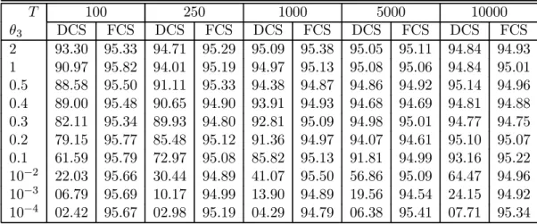
θ2 = 3.3andθ3 varies from2to0.0001; the sample sizeT is set toT = 100,250,1000,5000,and 10000. We construct 95%-level confidence sets for δ, using the delta method and the Fieller-type method. Based on 10000 replications, we compute the empirical coverage rate for both

procedures. Simulation results are shown in Table??.

These results show that the empirical coverage rate of the delta method based confidence

set deteriorates rapidly as the denominator becomes close to zero, no matter how large the sample size. Especially, when the denominator value is lower than 0.1, the empirical coverage

rate deviates markedly from the nominal confidence level. In contrast, the Fieller-type method,

although it is approximate in our application, does not suﬀer from such problems. The poor

performance of the delta method based confidence set might be more serious in many empirical

models where specified discret choice models are more complex. As a result, confidence sets

based on the delta method should be avoided, while the Fieller-type method is more appealing.

3.2.3 Simulation study II: a multinomial probit model with logit kernel

We consider a more complex formulation of discrete choice, i.e. the multinomial probit with

logit kernel model. Since the properties of standard asymptotics in this class of models are little

documented, it is important to assess the performance of both confidence set procedures within

this framework. The model can be described as follows.

Each individual denoted byn= 1, . . . , T in a population of sizeT faces J discrete alternatives

(or choices) of a choice set_C. The observed choice made by individualn is denoted by in ∈C,

and Xn is the (J × K) matrix of explanatory variables associated with individual n; these

variables include socio-economic variables, alternatives characteristics as well as diﬀerent types

(12)

Table 1: Empirical coverage rates for the delta method- and the Fieller method- based confidence sets for a parameter ratio in a simple binary probit model.

T 100 250 1000 5000 10000 θ3 DCS FCS DCS FCS DCS FCS DCS FCS DCS FCS 2 93.30 95.33 94.71 95.29 95.09 95.38 95.05 95.11 94.84 94.93 1 90.97 95.82 94.01 95.19 94.97 95.13 95.08 95.06 94.84 95.01 0.5 88.58 95.50 91.11 95.33 94.38 94.87 94.86 94.92 95.14 94.96 0.4 89.00 95.48 90.65 94.90 93.91 94.93 94.68 94.69 94.81 94.88 0.3 82.11 95.34 89.93 94.80 92.81 95.09 94.98 95.01 94.77 94.75 0.2 79.15 95.77 85.48 95.12 91.36 94.97 94.07 94.61 95.10 95.07 0.1 61.59 95.79 72.97 95.08 85.82 95.13 91.81 94.99 93.16 95.22 10−2 _22.03 _95.66 _30.44 _94.89 _41.07 _95.50 _56.86 _95.09 _64.47 _94.96 10−3 06.79 95.69 10.17 94.99 13.90 94.89 19.56 94.54 24.15 94.92 10−4 02.42 95.67 02.98 95.19 04.29 94.79 06.38 95.41 07.71 95.34

Note: Numbers reported are empirical coverage rates for the confidence set based on the delta

method [in the columns titled “DCS”] and for the one based on the Fieller’s method [in the

columns titled “FCS”]. θ3 is the denominator of the ratio andT is the sample size. The nominal

confidence level is 95%.

estimated is denoted by θ = (β0,β¯0)0, where the sub-vector β, of dimension (_{K ×}1), denotes

the parameters associated withXn and the sub-vectorβ¯ contains the nuisance parameters. We

write the discrete choice model for individualnas: ςi,n =

½

1 if individualnchooses alternative i

0 otherwise. (3.19)

Uin = Xinβ+εin, i= 1,2, . . . ,J, (3.20)

where Uin is the indirect utility indicator associated with alternative i for individual n. For

convenience, we write this model in the following compact form: Un=Xnβ+εn,

whereUn= (U1,n, U2,n, . . . , UJ,n)0 and εn= (ε1,n, ε2,n, . . . , εJ,n)0 areJ ×1vectors. For further

reference, let X denote the matrix that concatenates vertically the individual matrices Xn for

n= 1, . . . , T. The alternative i is chosen by individual n if and only if Uin ≥ Ujn,∀j ∈ C; the vectorςn= (ς1,n, ς2,n, . . . , ςJ,n)0 gives the observed choice made by individualn. Therefore, the choice probabilityPn(i) associated with the alternativei, i∈Cchosen by individualnis defined by:

Pn(i) =P(Uin ≥Ujn,∀j∈C). (3.21)

The computation burdens of the choice probability (3.21) depend on the distribution assumed

for the error term εn. For example, assuming εn

i.i.d.

(13)

(MNP) model. In this case Pn(i) requires the evaluation of multi-dimensional integrals, which may be analytically untractable for large choice sets; in particular, when the choice set involves

four or more alternatives, the choice probabilities are usually simulated. Assuming εn

i.i.d.

∼

Gumbel leads to the Multinomial Logit (MNL) model, in which case the choice probabilities have a simple to compute explicit form. In this simulation study, we consider the kernel logit model formulation that results from an attractive combination of MNP and MNL (see Ben-Akiva, Bolduc and Walker (2001)):

Un=Xnβ+εn (3.22)

εn=W ξn+νn,

W =F G, (3.23)

ξ_ni.i.d∼ N(0, I_J) and νni.i.d∼ Gumbel,

whereGis a diagonal matrix of dimension(_{J ×J})that have the standard deviation terms of the

componentsεnof its main diagonal, and the matrixF captures the correlation structure among

the error terms. Whenξ_n is known, this model reduces to the usual MNL model specification;

then the probability Pn(i) that individual n chooses alternative i conditionnally to ξn can be written as: Pn(i|ξn) = eXinβ+W_iξ_n J P j=1 eXjnβ+Wjξ_n . (3.24)

Then, we obtain the unconditional choice probability of alternative i by integrating Pn(i|ξn) over the domain ofξ_n:

Pn(i) = R _∞ −∞· · · R _∞ −∞ | {z } J Λ(i|ξ_n)n(ξ_n; 0, I_J)dξ_n. (3.25)

Expression in equation (3.25) shows that Pn(i) is a J-dimensional unbounded integral. In

our experiment, we consider _J = 3. So, we have been able to use numerical integration to

compute this tri-dimensional integral, athough it is very computer-time demanding. McFadden (1989) suggested the simulated maximum likelihood approach, where the multivariate integral is replaced by an approximation obtained by simulations. This approach requires draws from

the distribution ofξ_n. Using _S independent draws, the empirical mean

ˆ Pn(i) = 1 S S X r=1 Λ(i_|ξr_n), (3.26)

where ξr_n denotes a given draw r from the distribution of ξ_n, is an unbiased and consistent

estimator for the choice probability Pn(i). Then, replacing the choice probability in the log

likelihood with the simulatorPˆn(i) and maximizing the simulated likelihood function ˆ L(θ) = T X n=1 ln ˆPn(i|θ). (3.27)

(14)

lead to simulated maximum likelihood (SML) estimator. SML estimators are known to be

consistent and asymptotically eﬃcient under mild regularity conditions. Eﬃciency requires that

the sample size and the number of replications _S used to compute the probability simulator

both are large.

When estimating SML based logit kernel models, there may be two important problems

namely the non-identification of the parameter vector, and the bias associated with simulating

the log likelihood function. Walker (2001) highlights the fact that the Gumbel i.i.d.term leads

to extra identification conditions that impose restrictions on the matrices F and G. On the

other hand, using a large number of random draws _S helps reducing the simulation bias; for

instance Bolduc (1999) suggests that with _S = 50 draws, the estimation results are very close

to those obtained with a larger number of draws.

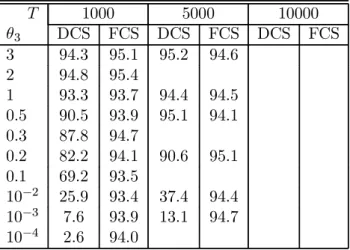
The model is estimated using the method of maximum likelihood. The choice probabilities Pn(i)are computed using the simulator defined by (3.26). The design of our simulation study is

as follows. Xn is composed of K= 5 variables that are drawn as 1.5 times independentU[0 1]

where U_[a _b] denotes the uniform distribution [a b], and _J = 3 alternatives. We consider

the ratio δ∗ = θ2/θ3. The parameters β of the utility indicator Un are set as follows: β =

(θ1, θ2, θ3, θ4, θ5)0 andθi= 3,fori= 1,2,4,5in all the experiment, whereasθ3, the denominator of the ratioδ∗ varies from3to0.0001. The sample sizeT is set toT = 1000,5000,and10000. For

the simulated choice probability method, we use_S = 50draws to evaluate the simulator (3.26),

while we use 12 integration points for the numerical integration method. We construct

95%-level confidence sets for δ∗, using the delta method and the Fieller-type method and compute

empirical coverage rates based on 1000 replications. Table 2 reports the empirical coverage rates for both procedures.

4 Simultaneous Con

fi

dence Sets for Multiple Ratios of

Parame-ters

Let us consider, in the context of model (2.1-2.2), s_≤p₋1 ratios of parametersρ_i, i= 1, ..., s

with a common denominator K0θ:

ρ_i=hi(θ) =L0iθ/K0θ,∀i= 1, ..., s, (4.28) where _{L1, L2, ..., Ls, K} is a linearly independent set of fixed (nonstochastic) p×1 vectors.5

Thesesratio functions have the same discontinuity set Dh defined by

Dh= ©

θ_∈Θ:K0θ= 0ª. (4.29)

Clearly,Dh 6=∅ sinceθ= (0, ...,0)∈Dh.

5_{Observe that if} _s

≥ p, then_{L1, L2, ..., Ls, K}are linearly dependent. Indeed, if s > p, then it is always

possible to express at leasts₋pelements of the set_{L1, L2, ..., Ls}as a linear combination of the others, and if

(15)

Table 2: Empirical coverage rates for the delta method- and the Fieller method- based confidence intervals for a parameter ratio in a kernel logit multinomial probit model.

T 1000 5000 10000 θ3 DCS FCS DCS FCS DCS FCS 3 94.3 95.1 95.2 94.6 2 94.8 95.4 1 93.3 93.7 94.4 94.5 0.5 90.5 93.9 95.1 94.1 0.3 87.8 94.7 0.2 82.2 94.1 90.6 95.1 0.1 69.2 93.5 10−2 _25.9 _93.4 _37.4 _94.4 10−3 7.6 93.9 13.1 94.7 10−4 2.6 94.0

Note: Numbers reported are empirical coverage rates for the confidence set based on the delta

method [in the columns titled “DCS”] and for the one based on the Fieller’s method [in the

columns titled “FCS”]. θ3 is the denominator of the ratio andT is the sample size. The nominal

confidence level is 95%.

We aim to construct simultaneous confidence sets for thesratios defined in (4.28) as well as for any linear combination of these ratios,

lw(ρ1, ρ2, ...ρs) = s X i=1

wiρi, (4.30)

wherew= (w1, w2, ..., ws)0 is any known nonstochastic (fixed) s×1 vector. We provide explicit solutions for these simultaneous confidence limits.

Zerbe et al. (1982) construct simultaneous confidence limits for several ratios of linear combi-nations of parameters in a normal linear regression model using an analysis of variance method

proposed in Scheﬀé (1959, 1953).6 They show that for each ratio, these confidence limits are

solutions to a quadratic equation and take the form (3.9). In addition, Zerbe et al. (1982) con-struct a joint confidence set for a finite number of ratios of linear combinations of regression

coeﬃcients with a common denominator and claimed that projections of this joint confidence

region on the individual ratios’ axes yield exactly the simulatneous confidence limits obtained

through the Scheﬀé’s method of analysis of variance.

In this section, we use results on quadric confidence sets (see Dufour and Taamouti (2003))

6_{In a normal linear regression model, this method gives simultaneous Wald type confidence sets for linear}

transfomations of a finite number of independent linear combinations of regression coeﬃcients. The method

applies to a ratio using a Fieller-type transformation, as in (3.7). It applies to the more general case where the ratios need not have the same denominator.

(16)

and derive simultaneous confidence limits for any linear combination of the s ratios defined in (4.28).

4.1 Joint con

fi

dence set for a

fi

nite number of parameters ratios

We define the followings linear combinations associated with the sratios ρ_i, i= 1, ..., s,as in (3.7): L0_iθ₋ρ_iK0θ= 0, i= 1, ..., s. (4.31) Let H = £ L1 . . . Ls K ¤0 _(4.32) R = · Is −ρ₁ . . . ₋ρ_s ¸0 ,

where Is is the s-dimensional identity matrix. The s×(s+ 1) matrix R has full row rank for

any possible values for ρ_i, i = 1, ..., s; and since the set of s+ 1 vectors _{L1, L2, ..., Ls, K} is

linearly independent, the matrixH has full row rank. Therefore, thesequations in (4.31) imply

snon-redundant restrictions that we write in the formRHθ = 0.

In order to obtain a joint confidence region for ρ= (ρ1, ..., ρs)0 we propose, as in Zerbe et al. (1982) and Young et al. (1997), to invert a Wald test for the restrictions

H0 :RHθ= 0. (4.33)

A(1₋α) level confidence region forρ,CS (ρ; 1₋α),is the set of all ρsuch that the latter test is not significant at levelα.

Let WRH denote the Wald statistic defined to test (4.33): WRH =

³

RHˆθ´0³RHΣˆˆ_θH0R0 ´−1³

RHˆθ´.

In our context,WRH has an asymptoticχ2(s) null distribution; letcα be the(1−α)percentile point of theχ2(s) distribution. Then, we defineCS (ρ; 1₋α) as:

CS (ρ; 1₋α) =_{ρ_∈_Rs:WRH ≤cα}. (4.34)

Zerbe et al. (1982) consider the following orthogonal decomposition that allows to characterize the analytical form ofCS (ρ; 1₋α):

WRH = ³ Hˆθ ´₀³ HΣˆˆ_θH0 ´₋1³ Hˆθ ´ − (4.35) ·_¡ ρ0,1¢ ³HΣˆˆ_θH0 ´−1 Hˆθ ¸0·_¡ ρ0,1¢ ³HΣˆˆ_θH0 ´−1¡ ρ0,1¢0 ¸−1·_¡ ρ0,1¢ ³HΣˆˆ_θH0 ´−1 Hˆθ ¸ . Substituting (4.35) in (4.34) and rearranging terms then yields:

(17)

where ρ_∗ =¡ρ0,1¢0 (4.37) M =c ³ HΣˆˆ_θH0 ´₋1 −·³HΣˆˆ_θH0 ´₋1 Hˆθ ¸ ·³ HΣˆˆ_θH0 ´₋1 Hˆθ ¸₀ c=³Hˆθ´0³HΣˆˆ_θH0 ´−1³ Hˆθ´₋cα. Therefore, (4.34) is written as:

CS (ρ; 1₋α) =nρ_∈_Rs:ρ0_∗M ρ_∗ _≤0, ρ_∗ =¡ρ0,1¢0o. (4.38)

The set CS (ρ; 1₋α) may take diﬀerent forms, which depend on whether the common

de-nominator of the ratios is statistically diﬀerent from zero or not [Scheﬀé (1970), Zerbe et al. (1982), Young et al. (1997)]: the interior of ans-dimensional ellipsoid, or a hyperboloid, or the

entire s-dimensional vector space _Rs_{. We use a theory of quadric con}_fi_{dence sets and derive}

explicit form for the projection-based simultaneous confidence sets for any scalar linear

trans-formation of the s ratios with common denominator, lw(ρ) = w0ρ, where w is a known fixed

(nonstochastic) vector.

4.2 Explicit solutions for simultaneous con

fi

dence sets for linear

transforma-tions of ratios

We characterize simultaneous confidence sets for linear transformations of a finite number of

ratios using the quadric confidence set theory, as developped in (Dufour and Taamouti (2003)).

The set of points that satisfy an equation of the formρ0Γρ+β0ρ+γ= 0,whereΓis a symmetric

s_×s matrix, β is a s_×1 vector and γ is a scalar, constitutes a quadric surface. A confidence

set forρof the form

Cρ = ©

ρ₀ :ρ0₀Γρ₀+β0ρ₀+γ_≤0ª

is a quadric confidence set (Dufour and Taamouti (2003)). Depending on the values ofΓ, β,and

γ,it may take several forms, including ellipsoids, paraboloids and hyperboloids.

The confidence set CS (ρ; 1₋α) defined in (4.38) can be written in the form of a quadric conficence set. Indeed, since ρ_∗ = (ρ0_,₁₎0_{, partition the matrix} _M _{accordingly in the form:}

M = · M11 M12 M21 M22 ¸ , (4.39)

where M11 is an s×s matrix, M12 is a s×1 vector, M21 = M120 , and M22 is a scalar. Let

S1 = (Is∼0s×1) be ans×(s+ 1) matrix andS2 = (0, ...,0,1)a 1×(s+ 1) vector. Then, the following relations hold:

ρ=S1ρ_∗, M11=S1M S10, M22=S2M S20.

(18)

The quadratic formρ0_∗M ρ_∗ is equivalently expressed as:

ρ0_∗M ρ_∗ =ρ0M11ρ+ 2M120 ρ+M22. Thus,CS (ρ; 1₋α) is written as the following quadric confidence set:

CS (ρ; 1₋α) =©ρ_∈_Rs:ρ0M11ρ+ 2M120 ρ+M22≤0 ª

. (4.40)

The joint confidence region CS (ρ; 1₋α) is multidimensional and may be hard to interpret

in practical applications. So, it is more convenient to derive confidence sets for individual

ratios or for scalar linear transformations of them. We apply the projection technique to the

quadric confidence setCS (ρ; 1₋α)(see Dufour and Taamouti (2003)) and obtain simultaneous

confidence sets for scalar linear transformations of the sconsidered ratios.

The projection technique is based on the following elementary probability result: given a

continuous fonctiong:Θ_→_Rq, q_≥1,and any subset E_⊂Θ, we have

∀x_∈Θ, (x_∈E)_⇒(g(x)_∈g(E)), where g(E) =_{y∈Rq:_∃ x∈E, g(x) =y}. This implies: ∀x_∈Θ, Pr [x_∈E]_≤Pr [g(x)_∈g(E)]. As a result, (Pr [ρ_∈CS (ρ; 1₋α)]_≥1₋α) =_⇒(Pr [g(ρ)_∈g(CS (ρ; 1₋α))]_≥1₋α).

This shows thatg(CS (ρ; 1₋α))is a confidence set for g(ρ)with level at least(1₋α); so, it is a conservative confidence set forg(ρ). More importantly, the projection-based confidence sets

obtained for any number of transformations g(ρ) of ρ are simultaneous, i.e. they satisfy the

inequality in (2.5). In particular, if we consider scalar linear transformations of ρ, lw(ρ) =w0ρ, w_∈_Rs,then the sets

CS¡w0ρ; 1₋α¢=©w0ρ₀:ρ0₀M11ρ0+ 2M120 ρ0+M22≤0 ª

(4.41) are simultaneous confidence sets for w0ρ, w _∈ _Rs_{. Special cases of linear combination include}

projections on the i-th component axe ρ_i of ρ, i = 1, ...s and these correspond to w = wi =

(δ1i, δ2i, ..., δsi)0, i= 1, ...s, where theKronecker delta δji is defined by δji =

½

1 when j=i 0 when j₆=i .

We can now characterize the explicit form of the projection-based confidence sets for scalar

(19)

Lemma 2 LetM11, M12, and M22 be defined by (4.37), (4.39). Then, M11 is nonsingular. In addition, let d=M₁₂0 M₁₁−1M12−M22. Thend >0 if and only if M11 is a positive definite or a negative definite matrix.

This result follows from the characterization provided by Zerbe et al. (1982, Appendix C)

for the geometric form of the multivariate confidence region (4.38). For convenience, we give in

the Appendix B the main steps of this characterization that are useful to establish Lemma 2. Let f =₋M₁₁−1M12, d=M120 M11−1M12−M22, (4.42) and let fi=− ¡ M₁₁−1¢_i.M12 be thei-th element off, _¡ M₁₁−1¢_i.

be thei-th row ofM₁₁−1,and _¡

M₁₁−1¢_ii

be the i-th element of the main diagonal of M₁₁−1. We can now state our main result in the

following theorem.

Theorem 3 Projection-based confidence sets for scalar linear transformations of ρ. Let M11, M12, M22, f and d be defined by (4.37), (4.39) and (4.42). Let the joint (1−α) level confidence set for ρ,CS (ρ; 1₋α), be defined as in (4.38)-(4.40). Let w _∈ _Rs_\{0_} and W11=w0M11−1w.

1. If all the eigenvalues of M11 are positive, then the projection-based confidence set for w0ρ defined by (4.41) corresponds to the bounded set

CS¡w0ρ; 1₋α¢=h w0f₋(dW11)1/2, w0f+ (dW11)1/2 i

. 2. If M11 has at least two negative eigenvalues, then CS (w0ρ; 1−α) =R. 3. If M11 has exactly one negative eigenvalue, then:

(a) If w0M₁₁−1w < 0, then the projection-based confidence set for w0ρ is a union of two unbounded sets: CS¡w0ρ; 1₋α¢= i −∞, w0f₋(dW11)1/2 i ∪ h w0f+ (dW11)1/2, +∞ h ; (b) If w0M₁₁−1w >0, thenCS (w0ρ; 1₋α) =_R. (c) If w0M₁₁−1w= 0,then CS (w0ρ; 1₋α) =_R\{w0f_}.

(20)

Proof. Since M11 is a real symmetric matrix, we have M11=G0D11G

whereGis an orthogonal matrix andD11is a diagonal matrix whose elements are the eigenvalues

of M11. Letλ1, λ2, ..., λs denote theseigenvalues of M11. Using the transformation z=G(ρ₋f),

the inequalityρ0₀M11ρ0+ 2M120 ρ0+M22≤0is equivalent to λ1z12+λ2z22+...+λszs2 ≤d. We may then write CS (w0ρ; 1₋α) as

CS¡w0ρ; 1₋α¢=©w0ρ₀ :λ1z12+λ2z22+...+λsz2s ≤d, z=G(ρ0−f) ª . SinceG0G=Is, we have w0ρ = w0G0Gρ = w0G0G(ρ−f) +w0G0Gf = w0G0[G(ρ₋f)] +w0f = v0z+w0f wherev=Gw. Define CS¡v0z; 1₋α¢=©v0z0 :λ1z12+λ2z22+...+λszs2 ≤d ª . (4.43) Then, forx_∈_R, £ x_∈CS¡w0ρ; 1₋α¢¤_⇔£x₋w0f _∈CS¡v0z; 1₋α¢¤.

The problem is then reduced to characterize CS (v0z; 1₋α). Clearly, the explicit form of CS (v0_z_{; 1}₋_α₎ _{depends on the number of negative eigenvalues of}_M₁₁_{. Then, the}

characteriza-tion results given in the Theorem obtain from Lemma 2 and Theorems 5.1-5.2 in Dufour and Taamouti (2003).

Theorem 3 characterizes the possible explicit forms for simultaneous projection-based con-fidence limits for scalar linear transformations of ρ from the joint confidence set defined in

(4.38)-(4.40). The explicit form depends on the number of negative eigenvalues of M11. From

the proof of Lemma 2 given in Appendix B, we see that the eigenvalues of M11 have the same

sign as cand a, where

c=³Hˆθ´0³HΣˆˆ_θH0 ´−1³

(21)

and a=c₋ · P0S1 ³ HΣˆˆ_θH0 ´₋1 Hˆθ ¸0· P0S1 ³ HΣˆˆ_θH0 ´₋1 Hˆθ ¸

wherec has multiplicitys₋1 and ahas multiplicity one.

Further, using Zerbe et al. (1982, Appendices C, D), it can be shown that a=³K0ˆθ ´₀³ K0Σˆˆ_θK ´₋1³ K0ˆθ ´ −cα. If _³ K0ˆθ´0³K0Σˆˆ_θK ´−1³ K0ˆθ´< c1,α (4.44) wherec1,α denote the (1−α) percentile point of the χ2(1) distribution, then the Wald test of H0 :K0θ= 0is not significant at levelα; the common denominator of the considered ratios may be arbitrarily close to zero. In this case, all the ratios ρ_i = hi(θ) = L0iθ/K0θ,∀i= 1, ..., s are near their discontinuity region defined in (4.29).

Further, ·³ K0ˆθ ´0³ K0Σˆˆ_θK ´−1³ K0ˆθ ´ < c1,α ¸ ⇒ ·³ K0ˆθ ´0³ K0Σˆˆ_θK ´−1³ K0ˆθ ´ < cα ¸ . Therefore, if ³ K0ˆθ ´₀³ K0Σˆˆ_θK ´₋1³ K0ˆθ ´ < c1,α and _³ Hˆθ ´₀³ HΣˆˆ_θH0 ´₋1³ Hˆθ ´ > cα

then a < 0 and c > 0, and as a consequence M11 has exactly one negative eigenvalue. The

individual ratios and any linear combination of them is almost unidentified, and this may cause

a level correct confidence set to be either unbounded or the entire real line.

On the other hand, if a > 0 and c > 0, which implies that all the eigenvalues of M11 are positive, then ³ K0ˆθ ´₀³ K0Σˆˆ_θK ´₋1³ K0ˆθ ´ > c1,α.

As a result, all the ratios and any linear combination of them are well-identified; this case

corresponds to bounded projection-based confidence set in Theorem 3.

The main point in Theorem 3 is that it gives easy-to-compute expressions for the confidence

limits for any linear transformationw0ρof the considered ratios, and not only for the individual ratios. It can be checked that for the individual ratios ρ_i, i= 1,2, ..., s, the simultaneous confi -dence limits given in Theorem 3 are numerically identical to the ones obtained by Zerbe et al. (1982).7 Specifically, for any individual ratioρ_i, i= 1,2, ..., s, the confidence limits are solutions to the following quadratic inequality:

Aiδ2i0+ 2Biδi0+Ci ≤0,

7_{This follows from the uniqueness of the projection on any individual}_ρ

(22)

where _         Ai = (K0θ)2−cα ³ K0Σˆˆ_θK ´ Bi = cα ³ L0 iΣˆˆ_θK ´ −(L0 iθ) (K0θ) Ci = (L0iθ) 2 −cα ³ L0_iΣˆˆ_θLi ´ .

The following corollary shows that the projection-based confidence set for any linear

trans-formation w0_ρ _{cannot be empty; as a special case, the simultaneous con}_fi_{dence sets for the}

individual ratios are non-empty sets.

Corollary 4 The simultaneous projection-based confidence sets defined by (4.41) for any number of scalar linear transformations of ratios with common denominator are non-empty sets. In particular, the simultaneous projection-based confidence sets for the individual ratiosρ_i, i= 1, ...s are non-empty.

Proof. From Dufour and Taamouti (2003), the only case where the projection-based con-fidence set for w0ρ is an empty set corresponds to: (i) M11 is positive definite and (ii) d <0. Using Lemma 2, this is impossible, and the result follows.

5 Empirical applications

In this section we illustrate the simultaneous confidence sets procedure discussed in the previous section through three empirical applications. The models we analyze are related to important

issues in transportation and energy economics. Thefirst one considers the trinomial logit model

of travel demand discussed by Ben-Akiva and Lerman (1985)8 in order to construct

simulta-neous confidence sets for the values of in-vehicle and out-of vehicle travel times. The second

one concerns inference for three values of travel time in multinomial probit models that com-bine maximum simulated likelihood (SML) estimator with Geweke-Hajivassiliou-Keane (GHK) choice probability simulator, in which cases standard asymptotics performs poorly. The third illustration is related to simultaneous inference for price- and income-elasticities in sector total energy demand models for the Province of Québec.

5.1 Value of time in trinomial logit model of travel demand

Estimating value of time is one important application of travel demand models with linear random utility. Although various theories of time allocation reveal that the value of travel time can be perceived in diﬀerent ways, most of empirical studies refer to the value of travel time as the amont of money the traveler agrees to pay in order to save one unit of the total duration of his travel [Ashton (1947), De Vany (1974), Truong and Hensher (1985), Bates (1987), Ben-Akiva, Bolduc and Bradley (1993)]. In a discrete choice framework, when the traveler’s utility fonction is specified as a linear function of travel cost, travel time and other variables, his evaluation of

8

We consider this model in section (3.2.1) for an illustration of confidence set procedures for one ratio of parameters.

(23)

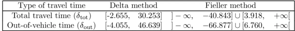
Table 3: Simultaneous confidence sets for values of total travel time and of out-of-vehicle time from Ben-Akiva and Lerman(1985)’s trinomial logit model, 95% nominal level.

Type of travel time Delta method Fieller method

Total travel time(δtot) [-2.655, 30.253] ]_{− ∞}, ₋40.843]_∪[3.918, +_∞[

Out-of-vehicle time (δout) [-4.055, 46.639] ]− ∞, −66.877]∪[6.760, +∞[

Notes: _ The delta method-based confidence intervals are not simultaneous.

the value of travel time is, up to a scalar constant, equal to the ratio of the coeﬃcient of the

time variable over the coeﬃcient of the cost variable [Truong and Hensher (1985), Bates (1987)].

We consider the trinomial logit model of travel demand from Ben-Akiva and Lerman (1985, Chapters 3, 5 and 7.). We have described this model in section 3.2.1. Here, we construct simultaneous confidence sets for the value of total travel time (δtot) and the value of out-of-vehicle time (δout) defined in equations (3.14) and (3.15) respectively. Using the notation of section 3.2.1, each of these values of travel time is a linear combination of the ratios functions h1(θ) =θ3/θ5 and h2(θ) =θ4/θ5 defined in model (3.12)-(3.13); so we can obtain Fieller-type

projection-based simultaneous confidence sets. We have also computed the delta method based

confidence sets for (δtot) and (δout), which are not simultaneous. We use sample average values for annual household income (equal to 12900$/year) and for one-way distance (equal to 810 centimiles). Our results are reported in Table 3.

5.2 Value of time in multinomial probit models in transportation

The second application we consider is, as the previous one, related to the economic value of time in discrete choice models. We consider results from the multinomial probit (MNP) model with correlated utilities estimated on a data bank on the choice of transportation modes for the morn-ing peak journey to work in the central business district of Santiago; for details on the model specification and the data see Bolduc (1999). Three specific uses of travel time are considered: in vehicle time, walking time and waiting time. The utility that a worker derives from his

jour-ney to work is assumed to be a linear function of transportation modes’specific dummies and of

other variables including cost/income, walking time, in vehicle time, waiting time, a sex dummy

and a dummy for no cars/no permit holders. This leads to three specific values of time that are

expressed as ratios of parameters with common denominator which is given by the coeﬃcient of

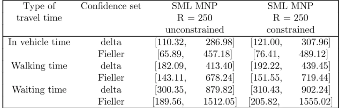
the variable cost/income. The estimation method combines the simulated maximum likelihood (SML) and the Geweke-Hajivassiliou-Keane (GHK) choice probability simulator based on ana-lytically computed scores. From the estimation results, Bolduc (1999) provided point estimates

for value of time ratios and standard delta method-based asymptotic t-statistics. Apply our

characterization results, we obtain simultaneous projection-based confidence sets for the three

value of time ratios. Tables ?? and ?? report the results along with the delta method-based

(24)

Table 4: Simultaneous confidence sets for values of time as percentage of net personal income, 95% nominal level.

Type of Confidence set MNP i.i.d. SML MNP SML MNP

travel time R = 50 R = 50

homoscedastic unconstrained

In vehicle time delta [117.90, 285.52] [122.07, 300.46] [102.69, 265.37]

Fieller [95.77, 352.52] [101.77, 382.24] [61.88, 411.03]

Walking time delta [240.79, 450.66] [239.39, 468.58] [178.65, 397.82]

Fieller [222.08, 548.30] [223.13, 590.17] [141.48, 631.17]

Waiting time delta [453, 1093.37] [507.58, 1201.34] [286.99, 830.65]

Fieller [370.12, 1350.40] [437.36, 1533.36] [178.70, 1373.47]

Note: _ The delta method-based confidence intervals are not simultaneous.

Table 5: Simultaneous confidence sets for values of time as percentage of net personal income,

95% nominal level (continued).

Type of Confidence set SML MNP SML MNP

travel time R = 250 R = 250

unconstrained constrained

In vehicle time delta [110.32, 286.98] [121.00, 307.96]

Fieller [65.89, 457.18] [76.41, 489.12]

Walking time delta [182.09, 413.40] [192.22, 439.45]

Fieller [143.11, 678.24] [151.55, 719.44]

Waiting time delta [300.35, 879.82] [310.43, 902.24]

Fieller [189.56, 1512.05] [205.82, 1555.02]

(25)

5.3 Price- and Income-Elasticities in total energy demand models

We consider a partial adjustment model of total energy demand for four sectors of energy use (industrial, commercial, residential and manufactured) in the Province of Québec. For each

sector, total energy demand depends on sector-specific explanatory variables and the model

is estimated with annual data set from 1962 to 2002. The demand equations are specified as

follows.

• For the residential sector:

ln (HTEt) = a0+a1ln (HTEt−1) +a2ln (PriceEt) +a3ln (HINCt) + (5.45) a4ln (DDHt)−a1a4ln (DDHt−1) +u1t

where for yeart, HTEt is average annual total energy demand per household, HINCt is

average annual disposable income per household,PriceEtis aggregate real price of energy,

DDHtis heating degree days.

• For the commercial sector:

ln (TECt) = b0+b1ln (TECt−1) +b2ln (PriceEt) +b3ln (GDPCt) + (5.46) b4ln (DDHt)−b1b4ln (DDHt−1) +u2t

where for yeart, TECt is total energy demand by the commercial sector, GDPCt is real

gross domestic product in the commercial sector.

• For the manufactured sector:

ln (TEMt) =c0+c1ln (TEMt−1) +c2ln (PriceEt) +c3ln (GDPMt) +u3t (5.47)

where for year t, TEMt is total energy demand by the manufactured sector, GDPMt is

real gross domestic product in the manufactured sector. • For the industrial sector:

ln (TEIt) =d0+d1ln (TEIt−1) +d2ln (PriceEt) +d3ln (GDPIt) +u4t (5.48) where for yeart,TEItis total energy demand by the industrial sector,GDPItis real gross domestic product in the industrial sector.

Convergence of the adjustment process for each sector requires 0 < a1 < 1, 0 < b1 < 1, 0 < c1 < 1, 0 < d1 < 1. The error terms u1t, u2t, u3t, u4t are assumed i.i.d. normal. The parameters of each equation are estimated using maximum likelihood estimator. The dynamic

specification of energy demand in (5.45)-(5.48) allows one to compute the long-run price and

income elasticities of sector energy demand. As an example, in the residential sector the long-run price elasticity_Erp is given by

Erp = a2 1₋a1

(26)

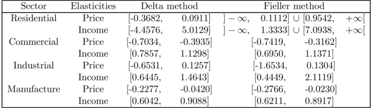
Table 6: Simultaneous confidence sets for long run price- and income- elasticities of total energy demand, nominal level: 95%.

Sector Elasticities Delta method Fieller method

Residential Price [-0.3682, 0.0911] ]_{− ∞}, 0.1112]_∪ [0.9542, +_∞[ Income [-4.4576, 5.0129] ]_{− ∞}, 1.3333]_∪ [7.0938, +_∞[ Commercial Price [-0.7034, -0.3935] [-0.7419, -0.3162] Income [0.7857, 1.1298] [0.6950, 1.1371] Industrial Price [-0.6531, 0.1257] [-1.6534, 0.1304] Income [0.6445, 1.4643] [0.4449, 2.1119] Manufacture Price [-0.2277, -0.0420] [-0.2766, -0.0230] Income [0.6042, 0.9088] [0.6211, 0.8917]

Note: _ The delta method-based confidence intervals are not simultaneous.

and the long-run income elasticity_Erinc is Erinc=

a3 1₋a1

. (5.50)

So, _Erp and Erinc are ratios of parameters with a common denominator and we can obtain

simultaneous confidence sets for _Erp and_Erinc. Table 6 reports simultaneous confidence sets for long run price-elasticities and income-elasticities for four sectors of energy use.

6 Conclusion

(27)

A

Appendix: Characterization of the solutions to the

Fieller-type con

fi

dence set for one parameters ratio

In this appendix, we characterize the Fieller-type confidence set for one parameter ratio. In the context of exact Fieller confidence sets, Scheﬀé (1970) gives such a characterization for the ratio of two means of normals and Zerbe et al. (1982) provides an extension to parameter ratio in normal linear regressions. Here, we extend these results to parameter ratio when the normal distribution of the estimator is only asymptotically justified.

Proposition 5 LetA, B, C be defined as in (3.11) and let∆=B2₋AC.Then, the(1₋α)-level Fieller-type confidence set FCS (δ; 1₋α) for the ratioδ =θ1/θ2, defined in (3.9), is character-ized as follows: 1. If ∆>0, then (a) if A >0, thenFCS (δ; 1₋α) = h −B−√∆ A , − B+√∆ A i , (b) else, ifA <0, thenFCS (δ; 1₋α) =i_−∞, −B− √ ∆ A i ∪h−B−A√∆, +∞ h . 2. If ∆<0, thenA <0 and FCS (δ; 1₋α) =_R.

Proof. We solve the equation

Aδ2₀+ 2Bδ0+C = 0 where _       A = ˆθ2₂₋z_α/22 ˆv2 B = ₋ˆθ1ˆθ2+z_α/22 ˆv12 C = ˆθ2₁−z_α/22 ˆv1

for real solutionsδ0. Except for a set of measure zero,A₆= 0,so we have a quadratic equation. Similarly, except for a set of measure zero,∆₆= 0; so we discuss the two cases where∆>0and ∆<0.Real solutions exist if and only if

∆>0.

If ∆>0,then we have two distinct real solutionsδ01 and δ02 given by δ01 = − B₋√∆ A δ02 = − B+√∆ A .

(28)

Therefore, FCS (δ; 1₋α) =        h −B−√∆ A , − B+√∆ A i if A >0 i −∞, −B−_A√∆i_∪i−B−_A√∆, +_∞i if A <0 .

To complete the proof, let us show that if∆<0, thenA <0. First, let us write∆as ∆=¡ˆv2₁₂₋vˆ1vˆ2 ¢ z_α/24 +³ˆθ2₁ˆv2+ ˆθ 2 2vˆ1−2ˆθ1ˆθ2ˆv12 ´ z_α/22 . Sincevˆ2

12−vˆ1vˆ2<0(Cauchy-Schwartz inequality), ∆is negative if and only if z∗= ˆθ 2 1ˆv2+ ˆθ 2 2vˆ1−2ˆθ1ˆθ2ˆv12 ˆ v1vˆ2−vˆ122 < z_α/22 . (A.51) From ˆ θ2₂/v2−z∗=− ³ ˆ θ2vˆ12−ˆθ1ˆv2 ´2 ˆ v2 ¡ ˆ v1vˆ2−vˆ122 ¢ , we get ˆ θ2₂/vˆ2−z∗<0. (A.52)

Then, from (A.51) and (A.52), we have

∆<0 _⇒ˆθ2₂/ˆv2 < z∗< zα/22 , which establishes that

∆<0_⇒A <0. Clearly, this implies

∆<0_⇒¡_∀δ0∈R,Aδ20+ 2Bδ0+C <0 ¢

(29)

B

Appendix: Proof of lemma 2

To prove Lemma 2, we need the following result known as the Sylvester’s law of inertia.

Lemma 6 (Sylvester’s law of inertia) Let Π1 and Π2 be any p×p symmetric matrices of the same rank r_≤p. If Π1 =NΠ2N0 for some matrix N, then Π1 and Π2 have the same number of positive eigenvalues.

Proof. (Lemma 6) Let us recall that the eigenvalues of any symmetric matrix are real

numbers. In addition, for any symmetric matrix Π, there exists an orthogonal matrix R (i.e.

R0 =R−1) such thatRΠR0 =D, whereD is a diagonal matrix with the eigenvalues of Πon its main diagonal.

Let λ(1)₁ , λ(1)₂ , ..., λ(1)p denote the p not necessarily distinct eigenvalues of Π1; similarly let λ(2)₁ , λ(2)₂ , ..., λ(2)p denote the eigenvalues ofΠ2, and let

D(1) = diag³λ(1)₁ , λ(1)₂ , ..., λ(1)_p ´ D(2) = diag ³ λ(2)₁ , λ(2)₂ , ..., λ(2)_p ´ ,

wherediag (a1, a2, ..., ap) denote the diagonal matrix witha1, a2, ..., ap as its main diagonal

ele-ments. Then, there exist two orthogonal matricesR(1) and R(2) such that

R(1)Π1R(1)0 = D(1) (B.53)

R(2)Π2R(2)0 = D(2). (B.54)

Let l1 and l2 be the number of positive eigenvalues of Π1 and Π2 respectively. Order the

eigenvalues of Π1 so that the first l1 scalars on the main diagonal of D(1) are positive and the next r₋l1 are negative; and do so forΠ2. This implies the following:

λ(1)₁ > 0, λ(1)₂ >0, ..., λ(1)_l 1 >0, λ(1)_l 1+1 < 0, λ (1) l1+2<0, ..., λ (1) r <0, λ(1)_r+1 = 0, λ(1)_r+2= 0, ..., λ(1)_p = 0; and λ(2)₁ > 0, λ(2)₂ >0, ..., λ(2)_l 2 >0, λ(2)_l 2+1 < 0, λ (2) l2+2<0, ..., λ (2) r <0, λ(2)_r+1 = 0, λ(2)_r+2= 0, ..., λ(2)_p = 0. Let D₁(1) = diag µq λ(1)₁ , q λ(1)₂ , ..., q λ(1)_l 1 ,− q −λ(1)_l 1+1, ...,− q −λ(1)r ,0, ...,0 ¶ D₁(2) = diag µq λ(2)₁ , q λ(2)₂ , ..., q λ(2)_l 2 ,− q −λ(2)_l 2+1, ...,− q −λ(2)r ,0, ...,0 ¶ .

(30)

DefineD(1)₀ and D₀(2) by: D(1)₀ =   Il1 0 0 0 ₋Ir−l1 0 0 0 0p−r   and D(2)₀ =   Il2 0 0 0 ₋Ir−l2 0 0 0 0p−r   Then we have: D(1) = U(1)D₁(1)D₀(1)D₁(1)U(1)0 (B.55) D(2) = U(2)D₁(2)D₀(2)D₁(2)U(2)0 (B.56)

whereU(1) andU(2) are permutation matrices and so they are orthogonal. Hence, substituting

(B.55) and (B.56) into (B.53) and (B.54) respectively, we obtain:

Π1 = R(1)0U(1)D(1)₁ D(1)₀ D(1)₁ U(1)0R(1) Π2 = R(2)0U(2)D(2)1 D (2) 0 D (2) 1 U (2)0_R(2)_. Then, we can writeD(1)₀ and D(2)₀ in the form:

D(1)₀ = P(1)Π1P(1)0 (B.57)

D(2)₀ = P(2)Π2P(2)0 (B.58)

whereP(1)=hR(1)0U(1)D(1)₁ i−1 and P(2) =hR(2)0U(2)D₁(2)i−1.

To prove the lemma, it suﬃces to show thatl1 =l2.Since Π1 =NΠ2N0, using (B.57) and (B.58) we get D(1)₀ =P(1)Π1P(1)0 =P(1)N µ³ P(2)´−1D(2)₀ ³P(2)0´−1 ¶ N0P(1)0 Let_z=P(1)N¡P(2)¢−1. Then D(1)₀ =_zD₀(2)z0. (B.59) Supposel2< l1. LetY = ¡ Y₁0,01×(p−l1) ¢₀ whereY1 = (y1, y2, ..., yl1) 0 _and _Y 16= 0.We have Y0D(1)₀ Y = l1 X i=1 y2_i >0. (B.60)

Now, partition_z0 in the form:

z0 = ·

z1 z2 z3 z4

(31)

where_z1 isl2×l1.Sincel2 < l1, the null space ofz1is not reduced to the null vector space and we can chooseY1 6= 0 so thatz1Y1 =0l2×1. Define z=z3Y1,and write z= (z1, z2, ..., zp−l2)

0_. Then we have_z0Y = (01×l2, z0) 0_{. Using (B.59), we obtain} Y0D₀(1)Y = ¡_z0Y¢0D(2)₀ ¡_z0Y¢ = ₋ rX−l2 j=1 z_j2 _≤0. (B.61)

Clearly, (B.60) and (B.61) are in contradiction; as a result,l2 < l1 is impossible.

Similarly, interchanging the roles ofD₀(1) andD₀(2), we can see thatl1< l2 is also impossible. Hence,l1=l2,and Lemma 6 is proved.

Proof. (Lemma 2) Since we assume that det³Σˆˆ_θ ´

6

= 0, the covariance matrix Σˆˆ_θ is sym-metric and positive definite. Then, since H has full row rank, it follows that ³HΣˆˆ_θH0

´−1 is symmetric and positive definite. Similarly, sinceS1 has full row rank, Q= S1

³

HΣˆˆ_θH0 ´−1

S₁0

is a symmetric and positive definite matrix. Then, there exists a nonsingular matrix P such

thatP0QP =Is.Using Lemma 6, the two matrices P0M11P and M11 have the same number of

positive eigenvalues and the same number of negative eignenvalues. In addition, we have: P0M11P =P0 ¡ S1M S10 ¢ P =P0 · S1 µ c³HΣˆˆ_θH0 ´−1 −·³HΣˆˆ_θH0 ´−1 Hˆθ¸ ·³HΣˆˆ_θH0 ´−1 Hˆθ ¸0¶ S₁0 ¸ P =cP0S1 ³ HΣˆˆ_θH0 ´−1 S₁0P₋P0S1 ·³ HΣˆˆ_θH0 ´−1 Hˆθ¸ ·³HΣˆˆ_θH0 ´−1 Hˆθ ¸₀ S₁0P =cIs− · P0S1 ³ HΣˆˆ_θH0 ´₋1 Hˆθ ¸ · P0S1 ³ HΣˆˆ_θH0 ´₋1 Hˆθ ¸₀ .

The last expression shows that P0M11P is a patterned matrix of the type discussed in Graybill

(1983, p. 206). Thus, P0_M₁₁_P _has₍_s₋₁₎_{eigenvalues equal to}_c _{and one eigenvalue equal to}

a=c₋ · P0S1 ³ HΣˆˆ_θH0 ´−1 Hˆθ ¸0· P0S1 ³ HΣˆˆ_θH0 ´−1 Hˆθ ¸ .

Except for a set of values forˆθof measure zero,c₆= 0and a₆= 0;so, zero is not an eigenvalue of M11 and M11 is nonsingular. The sign of det (M11) is the same as the sign of det (P0M11P) = acs−1_.

Similarly, using the same arguments as above for the matrix M, the sign of det (M) is the

same as that of ₋cαcs. In addition, using block matrix inversion formula, and since M22−

M21M11−1M12 is a scalar, we get:

det (M) = det (M11) det ¡ M22−M21M11−1M12 ¢ = ₋det (M11) ¡ M21M11−1M12−M22 ¢ = ₋det (M11)d,

Identification Robust Confidence Sets Methods for Inference on Parameter Ratios and their Application to Estimating Value-of-Time