Robust Methods for Program Evaluation.

(1)

Robust Methods for Program Evaluation

by

Nestor Sebastian Calonico

A dissertation submitted in partial fulfillment of the requirements for the degree of

Doctor of Philosophy (Economics)

in The University of Michigan 2014

Doctoral Committee:

Associate Professor Matias D. Cattaneo, Co-Chair Professor Jeffrey A. Smith, Co-Chair

Professor Richard A. Hirth Professor Lutz Kilian

(2)

c

Nestor Sebastian Calonico 2014

(3)

LIST OF FIGURES . . . iv LIST OF TABLES . . . v LIST OF APPENDICES . . . vi ABSTRACT . . . vii CHAPTER I. Identifying Distributional Effects of Teachers and Peers in Nonseparable Models . . . 1 1.1 Introduction . . . 1 1.2 STAR Project . . . 6 1.3 The Model . . . 10 1.3.1 Identification . . . 13 1.3.2 Implementation . . . 19 1.4 Empirical Results . . . 24 1.4.1 Class Size . . . 26 1.4.2 Teacher Experience . . . 28 1.4.3 Proportion of Females . . . 31

1.4.4 Tables and graphs . . . 33

1.5 Conclusion . . . 34

II. Robust Nonparametric Confidence Intervals for Regression-Discontinuity Designs . . . 39

2.1 Introduction . . . 39

2.2 Sharp RD Design . . . 43

2.2.1 Robust Local-Linear Confidence Intervals . . . 45

2.3 Other RD Designs . . . 52

2.3.1 Sharp Kink RD . . . 53

(4)

2.3.3 Fuzzy Kink RD . . . 57

2.4 Validity of MSE-Optimal Bandwidth Selectors . . . 58

2.4.1 Sharp Designs . . . 58

2.4.2 Fuzzy Designs . . . 60

2.5 Standard Errors . . . 61

2.6 Simulation Evidence . . . 63

2.7 Conclusion . . . 65

III. Optimal Data-Driven Regression Discontinuity Plots . . . 68

3.1 Introduction . . . 68

3.2 Setup and RD plots . . . 73

3.2.1 RD Plots . . . 75

3.3 Evenly-Spaced RD Plots . . . 78

3.3.1 Optimal Choice of ES Partition Size . . . 79

3.3.2 Data-Driven Implementations of JES,−,n and JES,+,n . 80 3.4 Quantile-Spaced RD Plots . . . 85

3.4.1 Optimal Choice of QS Partition Size . . . 86

3.4.2 Data-Driven Implementations of JQS,−,n and JQS,+,n . 88 3.5 Numerical Results . . . 90

3.5.1 Empirical Illustration . . . 90

3.5.2 Simulations . . . 92

3.5.3 Comparison of Partitioning Schemes . . . 96

3.6 Conclusions . . . 98

APPENDICES . . . 99

A.1 Appendix Chapter 1 . . . 100

B.1 Appendix Chapter 2 . . . 104

B.1.1 Local Polynomial Estimators and Other Notation . 104 B.1.2 Sharp RD Designs . . . 106

B.1.3 Fuzzy RD Designs . . . 108

B.1.4 Sharp RD Bandwidth Selectors . . . 111

C.1 Appendix Chapter 3 . . . 113

(5)

LIST OF FIGURES

Figure

1.1 Class Size - Policy I . . . 36

1.2 Class Size - Policy II . . . 36

1.3 Teacher Experience - Policy I . . . 37

1.4 Teacher Experience - Policy II . . . 37

1.5 Proportion of Females - Policy I . . . 38

1.6 Proportion of Females - Policy II . . . 38

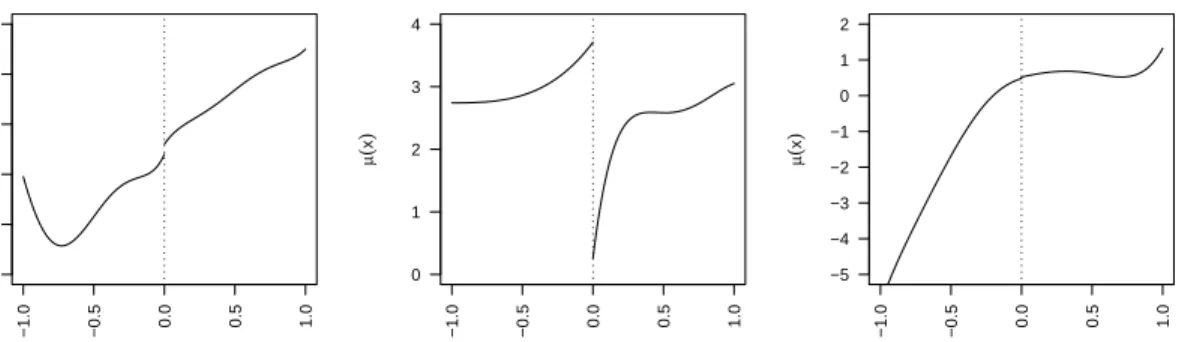
2.1 Regression Functions for Models 1–3 in simulations. . . 64

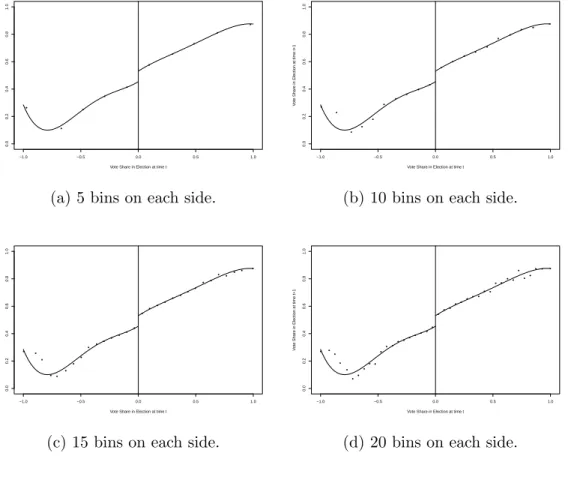
3.1 RD Plots - House Elections Data from Lee (2008). . . 71

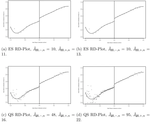
3.2 Optimal Data-Driven RD Plots for House Elections Data . . . 92

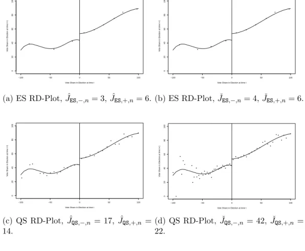
3.3 Optimal Data-Driven RD Plots for Senate Elections Data . . . 93

(6)

LIST OF TABLES

Table

1.1 Summary Statistics - Students . . . 33

1.2 Summary Statistics - Classrooms . . . 33

1.3 Class Size . . . 34

1.4 Teacher Experience - 5 to 10 years . . . 34

1.5 Teacher Experience - 10 to 15 years . . . 34

1.6 Proportion of Females . . . 34

2.1 Empirical Coverage and Average Interval Length of different 95% Confidence Intervals . . . 67

3.1 Data Generating Processes . . . 95

C.1 Simulations Results for Model 1 . . . 124

(7)

LIST OF APPENDICES

Appendix

A. Appendix to Chapter 1 . . . 100 B. Appendix to Chapter 2 . . . 104 C. Appendix to Chapter 3 . . . 113

(8)

ABSTRACT

Robust Methods for Program Evaluation by

Sebastian Calonico

My dissertation research focuses on different approaches to conduct robust estimation and inference in the context of program evaluation.

In Chapter 1, I look at the effects of teacher and peer characteristics on student achievement in the STAR Project conducted in Tennessee in the late 1980s. As in standard linear models, the proposed approach considers two types of unobservables: school-specific effects and idiosyncratic disturbances. It generalizes previous empir-ical research by allowing both effects to enter the structural function nonseparably. No functional form assumptions are needed for identification. Instead, it uses an exchangeability condition in the way that covariates affect the distribution of the school-specific effects. The model permits nonparametric distributional and counter-factual analysis of heterogeneous effects: it extends policy analysis beyond marginal or discrete changes to consider distributional effects originating from a counterfactual change in the distribution of characteristics of classrooms, peers and teachers. Also, these impacts can be analyzed on any feature of the distribution of student achieve-ment, such as quantiles and inequality measures. The empirical analysis looks at the effects of class size, teacher experience and gender composition of the classroom

(9)

on test scores. Findings suggest that nonseparable heterogeneity is an important source of individual-level variation in academic performance. The impact of class size is considerably larger using my approach: students in smaller classes benefit about 0.3 standard deviations, compared to a 0.16 effect obtained using a standard linear model. Also, teacher experience has a stronger, nonlinear impact. Still, the distri-butional analysis suggests that these gains are hard to achieve when facing resource constraints.

In Chapter 2, a joint work with Matias Cattaneo and Rocio Titiunik, we study robust inference in the context of regression discontinuity (RD) design. In the RD approach, units are assigned to treatment based on whether their value of an ob-served covariate exceeds a known cutoff. Local polynomial estimators are routinely employed to construct confidence intervals for treatment effects. The performance of these confidence intervals in applications, however, may be seriously hampered by their sensitivity to the specific bandwidth employed. Available bandwidth selectors typically yield a “large” bandwidth, leading to data-driven confidence intervals that may be severely biased, with empirical coverage well below their nominal target. We propose new theory-based, more robust confidence interval estimators for average treatment effects at the cutoff in sharp RD, sharp kink RD, fuzzy RD and fuzzy kink RD designs. Our proposed confidence intervals are constructed using a bias-corrected RD estimator together with a novel standard error estimator. For practical implemen-tation, we discuss mean-square error optimal bandwidths, which are by construction not valid for conventional confidence intervals but valid with our robust approach, and consistent standard error estimators based on our new variance formulas. Among other possibilities, our results give formal justification to simple inference procedures based on increasing the order of the local polynomial estimators employed. We find in a simulation study that our confidence intervals exhibit close-to-correct empirical coverage and good empirical interval length on average, remarkably improving upon

(10)

the alternatives available in the literature.

Finally, in Chapter 3, also written jointly with Matias Cattaneo and Rocio Titiu-nik, we present new results regarding RD plots. Exploratory data analysis plays a central role in applied statistics and econometrics. Specially in the RD approach, the use of graphical analysis has been advocated because it provides both easy pre-sentation and transparent validation of the design [e.g., Imbens and Lemieux (2008, Section 3) and Lee and Lemieux (2010, Section 4.1)]. RD plots are nowadays widely used in applications, despite its formal properties being unknown: these plots are typ-ically presented employing ad hoc choices of tuning parameters, which makes these procedures less automatic and more subjective. We formally study the most common RD plot based on an evenly-spaced binning of the data, and propose an optimal data-driven choice for the number of bins. This leads to an RD plot that is constructed objectively using the data available. In addition, we introduce an alternative RD plot based on quantile-spaced binning, study its formal properties, and propose the corresponding optimal data-driven choice for the number of bins. The main proposed data-driven selectors employ spacings-based estimators, which are simple and easy to implement in applications because they do not require additional choices of tuning parameters. Altogether, our results offer two alternative RD plots that are objective and automatic when implemented, thereby providing a reliable benchmark for em-pirical work using RD designs. We illustrate the performance of our automatic RD plots using two empirical applications and a Monte Carlo study.

(11)

CHAPTER I

Identifying Distributional Effects of Teachers and

Peers in Nonseparable Models

1.1 Introduction

The effects of educational inputs such as class size, teaching quality and school resources on student achievement have long been studied in the economic literature. In a highly influential work, Hanushek (1986) concludes that the literature does not provide strong evidence of a consistent relationship between school resources and stu-dent performance. A positive effect of school inputs, particularly teaching quality, has instead been highlighted in more recent work. For example, Card and Krueger 1992; 1996 find a positive relationship between school resources and student achieve-ment, showing that both low pupil-teacher ratios and high quality school systems lead to higher future earnings for students. Mixed conclusions have been reached on the effect of class size on student performance: while some studies conclude that small classes do not improve student achievement (e.g., (Hanushek, 2003), (Hoxby, 2000)), others find evidence of a positive impact (e.g., Krueger (1999), Krueger and Whitmore (2001), Angrist and Lavy (1999)).

These contrasting results have usually been attributed to econometric problems that make it difficult to recover the causal effect of educational inputs on student

(12)

performance, especially those related to omitted variable bias and reverse causality. Early studies have often relied on data in which the allocation of students to classes was not the result of an exogenous assignment. For example, schools might assign less able students to smaller classes, or better teachers to larger ones. In other cases, the allocation of students to classes is not exogenous due to parent decisions, for example parents more concerned about the education of their children may choose schools with a smaller class size or more experienced teachers.

With the aim to provide more reliable estimates, recent studies have relied on con-trolled randomized experiments or natural experiments. Most notably, a number of works have used data from the STAR Project, conducted in Tennessee from 1985-89. This was a large-scale, longitudinal experimental study of reduced class size, where students and teachers were randomly allocated to different class sizes. It motivated a large body of research on the effects of different classroom characteristics (not only class size, but also other factors such as teacher experience) on student performance both in the short and long-run. Most of the studies conclude that smaller classes in-crease student achievement, even after controlling for school fixed effects and teacher characteristics (e.g., Krueger (1999), Krueger and Whitmore (2001), Nye, Konstan-topoulos, and Hedges (2004)).

Besides relying on an experimental setting, a common feature of all these studies is that they are based on linear models, where we can account for unobserved school heterogeneity by including school dummies, which can be handled with standard lin-ear panel methods such as within-group transformations. I propose to extend this approach by considering a more general, nonseparable model that does not impose any functional form or parametric assumptions. In particular, no additivity or mono-tonicity assumptions are required for identification. Using the STAR Project data, I look at the influence of teacher experience, class size and gender composition of the classroom on student performance on standardized tests. The main motivation

(13)

behind this analysis is based on several important limitations of the standard model, which usually assumes a linear specification of the form:

Yics =µs+Pcsβ+Zics0 γ+εics (1.1)

where Yics is a measure of achievement (e.g., kindergarten test scores) for student

i assigned to classroom c in school s, Pcs is a classroom characteristic (e.g., class

size or teacher experience). Finally, Zics accounts for other student and teacher

characteristics that affect student performance. The main interest is on the parameter

β, e.g, the impact of class size or teacher experience on test scores. The model also includes two types of unobserved heterogeneity: a school fixed effect µs and an

individual specific component, εics.

The model presents several limitations, mostly derived from the linearity assump-tion. This is crucial for identification, since the school fixed effect µs is usually

differ-enced out. Besides being subject to model misspecification, this imposes important limitations for the analysis of heterogeneity in terms of the relationship between the impact of the covariates and µs. The marginal effect of Pcs onYics (e.g., a marginal

change in the gender composition of the classroom) is: ∂Yics/∂Pcs =β, or β(p1−p0)

for a discrete change (e.g., a reduction in class size). Given the additively separable assumption, the model fails to capture the heterogeneity that comes from µs, such as

unobserved school characteristics or other attributes that affect all members of the school but cannot be observed in the data. Additionally, it rules out the possibility

of heterogeneous treatment effects, which is often an important feature of the data

(e.g., Heckman, Smith, and Clements (1997) and Djebbari and Smith (2008)). For example, it does not account for the possibility that the effect of the same reduction in class size could be larger for schools with better reputations.

Additionally, the linearity assumption limits other aspects of the analysis. First, regarding what features of the distribution of student achievement are considered.

(14)

Usually the analysis focuses on average outcomes; that is, the effects on the condi-tional expectation of Yics. Heterogeneity is most commonly accounted for by looking

at subgroup impacts based on demographic characteristics. A small number of stud-ies also look at quantile treatment effects (e.g., Jackson and Page (2013)), but the inclusion of fixed-effects is not straightforward as they can no longer be differenced out and additional assumptions are required. Second, it also limits the type of pol-icy analysis that can be conducted. In a linear model, β measures the impact of a marginal or discrete change in Pcs. This might not be very informative in terms

of policy implementation. For example, if we care about reallocations of individuals across groups as opposed to infeasible increases in the population. These realloca-tions can be characterized by obeying a particular feasibility constraint that should be accounted for. For example, one might be interested on the distributional effects of a policy that reduces gender segregation in the classroom, while keeping the total number of students of both genders fixed.

I propose a general method trying to account for these limitations. First, I use a nonseparable model of the form:

Yics =m(µs, Pcs, Zics, εics).

where them(·) function is assumed unknown and left completely unspecified. Nonsep-arable models have been widely studied in the econometrics literature (e.g., Matzkin 2007; 2013). In the model I employ, no additivity or monotonicity assumptions are required for identification of certain parameters related to the effect of teacher and peer characteristics on student achievement. In addition, both µs and εics can be of

any dimension and interact with the covariates in general ways, in particular allowing

(15)

∂Yics

∂Pcs

= ∂m(p, z, µ, ε)

∂p .

Now the effect is allowed to be different even for students with the same observed characteristics. The same is true for a discrete change:

m(µs, p1, Zics, εics)−m(µs, p0, Zics, εics)

The method I propose goes beyond the effect of marginal and discrete changes of the covariates. In particular, I extend the analysis to consider counterfactual changes in the marginal distribution ofPcs, and their effect on the unconditional distribution

of the outcome. For example, my method allows me to study the effects of a policy that modifies the distribution of teacher experience by reducing the number of less experienced teachers. Additionally, the impact of these counterfactual policies can be identified on any feature of the distribution of Yics. This includes, for example, the

mean, quantiles and other functionals such as inequality measures.

The identification strategy is based on a control function approach that disen-tangles the direct effect of Pcs on Yics by keeping the distribution of unobservables

fixed. The main concern is the possible correlation between the school fixed effects

µs and the policy variable Pcs. This is handled via an exchangeability assumption

(Altonji and Matzkin (2005)) on the conditional distribution of µs given observable

class characteristics, which imposes that they cannot be ordered in a particular way in each school.

Using data from the STAR Project, I look at the influence of class size, teacher experience and gender composition of the class on test scores. My findings suggest that nonseparable heterogeneity is an important source of individual-level variation in the academic performance of kindergarten students. Using the nonseparable model, the impact of class size is considerably larger: students in smaller classes benefit

(16)

about 0.3 standard deviations, compared to a 0.16 effect obtained with a linear model. Also, teacher experience has a stronger, nonlinear impact: students assigned to more experienced teachers perform better in standardized test scores, and the gain increases with years of experience. Still, conducting a counterfactual distributional analysis I find that these gains in student performance are hard to achieve when facing resource constraints. For example, I find that a policy that reduces the size of some classes while keeping the number of students and teachers fixed generates a lower impact on test scores.

The remainder of the chapter is organized as follows. Section 2 describes the STAR Project and discusses some of the related literature. Identification, estimation and implementation of the proposed model are discussed in Section 3. Section 4 presents my empirical findings, comparing them with previous approaches. Finally, I discuss the main conclusions in Section 5. Proofs to the theorems are included in the appendix.

1.2 STAR Project

The Student/Teacher Achievement Ratio (STAR) Project was conducted in Ten-nessee during 1985-89. It was a large-scale, 4-year, longitudinal, experimental study of reduced class size, where students and teachers were randomly assigned to classes of different sizes. It included 79 schools from inner-city, rural, urban, and suburban locations, and over 6,000 students per grade level (for students in kindergarten and grades 1 to 3).

A large body of research has looked at the relationship between class size and student performance in nonexperimental settings, but the STAR Project was the first large-scale experiment to address this issue. In the absence of an experiment, the effect of a policy may be confounded by other observed or unobserved factors that may be correlated with the policy. In this case, the experiment only manipulated

(17)

class size and did not provide additional teacher training, new curriculum, or any other intervention.

In the original implementation of the experiment, students were to remain with the same randomly assigned class type from kindergarten through the end of the third grade. In practice, however, there were several deviations. Students who en-tered a participating school after the first year of the program were added to the experiment and randomly assigned to a class type. There was a substantial number of new entrants: 45 percent of eventual participants entered after kindergarten, due in part because, at the time, kindergarten was not required in Tennessee. A relatively large fraction of students exited the STAR Project schools (45 percent of overall par-ticipants) due to school moves, grade retention, or grade skipping. In addition, in response to parental concerns about fairness to students, all students in regular and regular-aide classes were randomized again in the first grade. Finally, a smaller num-ber of students (about 10 percent of participants) were moved from one type of class to another in a nonrandom manner. Most of these moves reportedly were due to student misbehavior and not typically the result of parental requests to move their child to a small class. Still, if families felt that their child would be better served by attending smaller classes (or were upset that their child was randomly assigned to a regular class), this might yield a differential attrition rate or better attendance rate by class type. For these reasons, in this chapter I focus only on the sample of students who entered the project in kindergarten.

Ideally one would check randomization with a pretest to ensure that there are no measurable differences in the dependent variable by class type before the program began. Unfortunately, no baseline survey was collected. Still, several authors (e.g., Krueger (1999)) investigated this issue by comparing student characteristics that are related to student achievement but cannot be manipulated in response to treatment, such as student race, gender and age, finding no systematic differences in observable

(18)

characteristics across class type. Another drawback is that initial random assignment was not recorded, but instead initial enrollment was measured. This could be a concern if, for example, parents successfully lobbied for a class change in the days between class assignments and the beginning of school. Krueger (1999) presented evidence from a subset of the data suggesting that this was very unlikely. Finally, it is also important that teachers were randomly assigned. If the most effective teachers were disproportionately placed with small (or regular) classes, then the class-size effect would pick up this effect as well. Based on the data available, Krueger (1999) finds no observed within-school differences across observed characteristics of teachers, such as race, gender, experience level, or highest level of education.

In terms of external validity, there are a few aspects of the sample that may limit the validity of generalizing the STAR Project findings to other settings. In order to be eligible to participate in the program, schools were required to have a minimum-size cohort of fifty-seven students, enough to sustain both a regular and a regular-aide classroom of twenty-two students and one small class of fifteen students. As a result, the schools that participated were about 25 percent larger, on average, than other Tennessee schools. Because of requirements imposed by the legislature for geographic diversity, schools in inner cities were overrepresented, and the students included were more economically disadvantaged and more likely to be African-American than those in the state overall. Even though the percentage of non-white participants closely mirrors the percentage in the United States overall (33 versus 31 percent), there were very few Hispanic and Asian students in Tennessee at the time compared to the rest of the nation. Finally, average school spending in Tennessee was about three-fourths of the nationwide average, and teachers were less likely to have a master’s degree. Krueger (1999) and Schanzenbach (2006) provide additional details on the implementation of the programs.

(19)

quality, and peer characteristics have significant (both in a statistical sense and in magnitude) causal impacts on test scores (e.g., Schanzenbach (2006)). In addition, there is a large literature about their long-term impacts. Krueger (1999) finds that, on average, performance on standardized tests increases by four percentile points the first year students attend small classes, and this advantage expands by about one percentile point per year in subsequent years. The effects are larger for minority students and those on free/reduced lunch programs. Other studies have shown that students assigned to small classes are more likely to complete high school Finn, Gerber, and Boyd-Zaharias (2005), take the SAT or ACT college entrance exams and less likely to be arrested (Krueger and Whitmore (2001)).

Chetty, Friedman, Hilger, Saez, Schanzenbach, and Yagan (2011) analyze the long-term impacts of the STAR Project on college attendance, earnings, retirement savings, home ownership, and marriage by linking the original data to administrative data from tax returns.

More recently, Dynarski, Hyman, and Schanzenbach (2011) also find that students in small classes are more likely to enroll and complete college. However, very few studies look at distributional impacts beyond subgroup analysis in the STAR Project. Jackson and Page (2013) find heterogeneity across achievement quantiles, with the largest test score gains being at the top of the achievement distribution.

I contribute to this literature by providing a nonparametric, distributional evalua-tion of the impact of teachers, peers, and other class attributes on student performance in standardized tests. By looking at the effect of some classmate characteristics, the approach also relates to the peer effects literature, in particular to “contextual” effects models as described in Manski (1993).1

1_{See, e.g., Durlauf (2004) and Sacerdote (2011) for reviews, and Bramoulle, Djebbari, and Fortin} (2009), Boucher, Bramoull´e, Djebbari, and Fortin (2012) for recent empirical applications.

(20)

1.3 The Model

The performance on a standardized test for student i in classroom cfrom school

s, Yics, is assumed to be generated through the nonseparable model:

Yics =m(µs, Pcs, Zics, εics) (1.2)

fori= 1,· · · , Ics,c= 1,· · · , Csands= 1,· · ·, S, where (Pcs, Zics) is adx-dimensional

vector of covariates, with Pcs a scalar that could be any classroom, teacher or peer

characteristic whose effect on test scores we want to study. This flexible specification allows for general types of interaction between µs and Pcs, since no assumption is

made on the functional form ofm(·). This could be either a structural equation that describes the causal relationship between the variables, or a reduced form equation from a general structural system.

I consider several features of the relationship between test scores Yics and the

class charateristic Pcs. First, I look at two parameters that have a straightforward

interpretation and can be compared to the β coefficient from the linear model (1.1):

aWeighted Average Derivative Function for continuous variables Pcs, and a Discrete

Changes Function that evaluates Pcs at different points, useful for discrete random

variables such as class size or teacher experience. Finally, I introduce aCounterfactual

Distribution Function that measures the effect of general changes in the distribution

of Pcs on the marginal distribution of Yics.

Definition I.1. When m(µ, p, z, ε) is differentiable in p and p is continuously dis-tributed, the Local Average Response is:

δics(p, z) =

Z _∂m₍_{p, z, µ, ε}₎

∂p dFµs,εics|Pcs,Zics(µ, ε|p, z) (1.3) where Fµs,εics|Pcs,Zics(µ, ε|p, z) is the distribution function of (µs, εics) conditional on

(21)

Pcs =p and Zics=z.

That is,δics(p, z) is the partial effect ofPcs on the expected value ofYics, evaluated

at given values of Pcs and Zics, averaged over the distribution of unobservables. For

example, this could measure the average effect on test scores of a marginal change in the gender composition of the class, when the proportion of females is 0.5. Note that, without assumptions on the dependence relationship among students, classrooms and schools, the average derivative function is indexed by (i, c, s). I will discuss this issue in more detail in Section 3.2.

One concern with the Local Average Response is that most common nonparamet-ric estimators of (1.3) will exhibit low rates of convergence, especially when Zics is

high-dimensional. Besides, in some contexts the objective of the analysis is not to predict the entire derivative curve of a conditional expectation function at each data point. Instead, we might be interested in an average version of (1.3) over all values of (Pcs, Zics). Then, I also consider Weighted Average Derivatives.

Definition I.2. The Weighted Average Derivative Function is

δ_icsω =_E ∂m(p, z, µ, ε) ∂p ω(p, z) (1.4)

where ω(p, z) is some specified weight function.

The weighted average derivative function is a well known parameter, and its iden-tification and estimation have been extensively studied in the nonparametric and semiparametric literature, in part because it is possible to construct nonparametric estimators of (1.4) that attain parametric convergence rates. Certain regularity con-ditions are usually required on the regression functions, the data and the weights ω, such as compact support on (Pcs, Zics), bounded higher moments of Yics and

deriva-tives of them(·) function. See, e.g., Cattaneo, Crump, and Jansson (2010), Cattaneo, Crump, and Jansson (2013a), Cattaneo, Crump, and Jansson (2013b) and references

(22)

therein for a more detailed discussion. Also, see Newey and Stoker (1993) for effi-ciency results for average derivative estimators. I discuss implementations issues of (1.4) in section 3.2.

For discrete variables such as class size or years of teacher experience, we are instead interested in finite changes rather than infinitesimal ones. In this case, we can use:

Definition I.3. A Discrete Changes Function

∆ics(p00, p0) =

Z

[m(p00, z, µ, ε)−m(p0, z, µ, ε)]dFZics,µs,εics|Pcs(z, µ, ε|p

0

) (1.5)

is defined for a change betweenPcs =p00 toPcs =p0.

Finally, I discuss a Counterfactual Distributions Function that measures the effect of a counterfactual change in the distribution of Pcs on the marginal distribution of

Yics. The parameter of interest in this case is:

Definition I.4. The Counterfactual Distribution Function

FY∗

ics(y)≡P[m(µs, P

∗

cs, Zics, εics)≤y] (1.6)

is the marginal distribution of Y_ics∗ ≡m(µs, Pcs∗, Zics, εics) obtained by evaluating the

function m(·) at valuesP_cs∗, where the distribution ofPcs changed from FPcs toFPcs∗. Now the research question is: how would the unconditional distribution of student performanceYics change if a policy maker could exogenously shift the values ofPcs to

some P_cs∗, i.e., what is the difference between the distribution of Yics and that of the

counterfactual random variable Y_ics∗ . This new distribution can be obtained in differ-ent ways. For example, it could come from a transformation of the original random variable (such as a policy that consists of reducing the number of less experienced teachers), or from a different population (e.g. the distribution of teacher experience

(23)

from another state, different demographic groups or time periods, etc.). This type of counterfactual analysis have been extensively studied in other areas of economics (see, e.g., Fortin, Lemieux, and Firpo (2011)).

Note also that P_cs∗ can be dependent or independent of Pcs. Both cases can be

considered in the same framework, with only different implications in terms of im-plementation, as I discuss in the next section. Finally, the proposed approach also works for the case in which Pcs is different for each student, Pics. For example, Dee

(2004) looks at the effect of attending a class with teachers of similar characteristics as the students. Also, it does not have to consist only of classroom means (e.g. av-erage age of peers). Glewwe (1997) points out the limitations associated with using the mean of peer characteristics without taking into account their overall distribu-tion and how failure to do so can yield seriously misleading results. For example,

Pics = I−1PI i=1Z 1−ζ ics 1−ζ

accounts for other characteristics of the distribution ac-cording to the parameter ζ.

In all cases, the object of interest is the distribution FY∗

ics and how it compares to

FYics. The difference between them is called a distributional policy effect. In general, this approach can be used to conduct inference onFY∗

ics as a whole, its moments and quantiles, or some functionals of it, such as inequality measures. The next section discusses the assumptions required for identification of all three parameters.

1.3.1 Identification

The main identification concern is the possible correlation between Pcs and µs.

There are basically two ways in which Pcs affects Yics: a direct effect through the

function m(·), and an indirect effect through the distribution of µs. In a linear

approach, one could simply remove the effect of µs by differencing it out. This is no

longer possible in a nonseparable model, so additional assumptions are required. In particular, I assume the existence of a vector Vs including information at the school

(24)

level, such that the school fixed effect is independent ofPcs once we condition on Vs.

Then, we can isolate the direct effect ofPcs onYics. For example, one approach would

be to rely on a selection on observables type of assumption, and then construct theVs

vector with a rich set of school characteristics. Instead, I employ an exchangeability assumption that fits well in the context of the STAR Project. I develop this idea in more detail in the next section. For identification purposes, it is only required that the vector Vs satisfies:

Assumption I.5. µs⊥(Zics, Pcs)|Vs

Note that Vs has the role of a control function, and there could be many choices

of Vs satisfying this condition, each implying different restrictions on the model (see,

e.g., Matzkin 2007; 2013 and references therein). I discuss a particular strategy to construct Vs in Section 3.1.1. The main idea is that, by controlling for Vs, I can

isolated the direct effec of Pcs on Yics without the influence of µs.

The next assumption refers to the individual specific heterogeneity, εics. In the

context of the STAR Project, the random allocation of teachers and students to classroom ensures that εics⊥Pcs. For example, letεics represent family involvement

in their children’s education. Given random assignment of students and teachers into classrooms, it is expected that this student-specific characteristic is uncorrelated with the class size assigned to the student. More generally, I allow the independence of

εics and Pcs to be conditional:

Assumption I.6. εics ⊥Pcs|(µs, Zics, Vs)

The first two assumptions are sufficient for identification of the average derivative and discrete changes functions, and have been previously proposed in a similar context by Altonji and Matzkin (2005). The result is given in Theorems 1 and 2.

(25)

Theorem I.7 (Identification of Weighted Average Derivatives). Under (A.1)-(A.2): δ_icsω =_E ∂_E(Yics|Pcs =p, Zics=z, Vs =v) ∂Pcs ω(p, z) (1.7)

which also requires _E[|∂_E(Yics|Pcs =p, Zics=z, Vs =v)/∂Pcs|]<∞.

The idea behind the identification of δω

ics is straightforward. First, we calculate

the partial effect ofPcs onYics holdingVsconstant. This holds the distribution of

un-observables constant. Second, we compute the conditional distribution ofVs|Pcs, Zics

and recover δics(p, z) by integrating out Vs. From this result, identification of the

density weighted average derivatives follows directly by integrating over the joint dis-tribution of (Pcs, Zis). A similar identification strategy can be used for the discrete

changes function:

Theorem I.8 (Identification of Discrete Changes). Under (A.1)-(A-2):

∆ics(p00, p0) =

Z

E(Yics|Pcs =p00, Zics =z, Vs =v)dFZics,Vs|Pcs(z, v|p

0

) (1.8)

− _E(Yics|Pcs =p0)

The next two assumptions are specific to the counterfactual distribution analysis, and concern the type of distributions that can be considered for P_cs∗. A general assumption regarding the relationship between the counterfactual random variable and the unobservables is:

Assumption I.9. µs⊥(Zics, Pcs, Pcs∗)|Vs and εics ⊥(Pcs, Pcs∗)|(µs, Zics, Vs)

This would be satisfied, for example, if P_cs∗ is originated from a transformation of

Pcs, Pcs∗ = Γ(Pcs). Finally, I also impose a common support condition: Assumption I.10. sup(P_cs∗)⊆sup(Pcs)

(26)

This is required to achieve nonparametric identification due to the inability to extrapolate beyond the range observed in the data, restricting the policy experiments that can be considered to ones for which there is already some experience in the data. It could still be possible to give meaningful bounds on the counterfactual distribution when P_cs∗ is allowed to take values outside of the support of Pcs with

moderate probability. Identification follows:

Theorem I.11 (Identification of Counterfactual Distributions). Under (A.1)−(A.4):

FY_ics∗ (y) = E FYics|Pcs,Zics,Vs(y , P ∗ cs, Zics, Vs) (1.9)

That is, we can identify the unobserved marginal distribution of Y_ics∗ by first computing the conditional CDF of Yics given Pcs, Zics and Vs. As in the previous

cases, holding Vs holds the distribution of the fixed effects constant. Finally, the

unconditional distribution can be obtained by integrating over the distribution of (P_cs∗ , Zics, Vs). Also note that, from these results, functionals such as quantiles and

inequality measures are also identified.

Remark I.12. In all cases, an implicit assumption is the nonparametric identification

of the regression function _E(Yics|Pcs, Zics, Vs) for values of (Pcs, Zics, Vs) for which the

conditional density of (Vs, Zics) givenPcs is positive. I discuss this issue in more detail

in Section 3.1.1, after introducing the choice of Vs.

The methodological contribution of this chapter is to extend some previous re-sults from the literature on distributional counterfactual effects and on nonseparable models, especially some recent contributions in a panel data context. Rothe 2010; 2012 proposes a nonparametric procedure to analyze counterfactual distributions us-ing nonseparable models, but without accountus-ing for group-invariant fixed effects. Recently, Chernozhukov, Fern´andez-Val, and Melly (2013) consider policy interven-tions that correspond to either changes in the distribution of covariates, or changes

(27)

in the conditional distribution of the outcome given covariates, or both. This idea also contributes to research on nonseparable models, especially to some recent work for panel data. For a review of earlier contributions in a cross-sectional context, see Matzkin 2007; 2013. One important difference is that these models usually focus on the identification of local average structural derivatives (LASD), for which addi-tional assumptions are required. For example, monotonicity on the unobservables (e.g., Altonji and Matzkin (2005), Evdokimov (2010)). Su, Hoderlein, and White (2010) discuss several limitations of this assumption. Alternatively, other papers re-strict the analysis to a subpopulation for which the covariates do not change over time (e.g., Hoderlein and White (2012), Chernozhukov, Fern´andez-Val, Hahn, and Newey (2013)). None of these assumptions are employed in the identification results in Theorems 1 to 3.

1.3.1.1 Exchangeability

To find a vector Vs satisfying (A.1) I use the notion of exchangeability, first

intro-duced in the nonseparable models literature by Altonji and Matzkin (2005). Graham, Imbens, and Ridder (2010) also use an exchangeability assumption but at the stu-dent level, and in a different model, to study segregation by gender in kindergarten. Without loss of generality, I assume that there are two classrooms for each school,

C = 2. In the present context, exchangeability is defined as:

Definition I.13. The conditional distribution of µs given (X1s, X2s) is exchangeable

in (X1s, X2s) if Fµs|X1s,X2s(µ|x1, x2) = Fµs|X1s,X2s(µ|x2, x1), where Xcs = (Pcs, Zcs) is a vector of classroom characteristics.

This means that the conditional distribution Fµs|X1s,X2s(µ|x1, x2) is invariant to permutations of its arguments. That is, the subscript c is uninformative, and the information that (X1s, X2s) provides is independent of the order in which the elements

(28)

classrooms cannot be ordered in a particular way for all schools. The order could be natural in other contexts, such as in panel data (if, for example, we were following classroom over time). In that context, it rules out any type of dynamic behavior. Here I assume that there are no a priori reasons for the first classroom to have a different effect than the second one on the distribution of µs. An important restriction is the

implication that the same equality holds for any subset of the data.2 ForC = 2 this implies Fµs|X1s(µ|x1) = Fµs|X2s(µ|x2) which means that observable characteristics of each classroom provide the same information regarding the distribution of the school fixed effects. As opposed to a conditional independence assumption where we need to find a rich enough set of variables to include inVssuch that Assumption 1 is satisfied,

the exchangeability assumption can hold for any of the elements in Xcs.

Example I.14. Let µs ∈ {H, L}, so schools can be either low or high quality type.

Also, Xcs ∈ {1,2} represents years of teacher experience. One possible scenario

where the exchangeability assumption would not hold is when high quality schools always assign more experienced teachers to classroom 1. Then, it might be that

P(µs =H|X1s = 1, X2s = 2) = 0 whileP(µs =H|X1s = 2, X2s = 1)>0.

Example I.15. Suppose classrooms are numbered by the extend of external dis-traction (e.g., nice views out the window, external noise, broken chairs, etc). Then, teacher assignment should be invariant to these choices.

Example I.16. We can also gain some intuition by looking at types of distribu-tional assumptions that would lead to exchangeability. Let Pcs = Ps + Pecs and

µs =θPs+µes, where Ps v N(0,1), Pecs vN(0,1), and µes v N(0,1), all i.i.d. Then,

Fµs|P1s,P2s(µ|p1, p2) =Fµs|Vs(µ|p1+p2) by properties of the normal distribution. To sum up, exchangeability is a reasonable assumption in the context of the STAR Project, where teachers and students were randomly assigned to each classroom,

(29)

which, even though classrooms were of different size, this is observed and can be accounted for by including class size as one of the elements of Xcs. This assumption

can be used to construct a vectorVssatisfying (A.1). First, the Fundamental Theorem

of Symmetric Polynomial Functions states that any symmetric polynomial can be written in terms of elementary symmetric functions. Together with the Weierstrass approximation theorem, this implies that if Fµs|X1s,X2s(µ|x1, x2) is exchangeable in (X1s, X2s), it can be approximated arbitrarily close by a function of the form:

Fµs|X1s,X2s(µ|x1, x2) = Fµs|Vs(µ|v) (1.10)

whereVs≡(Vs1, Vs2) are elementary symmetric polynomials of (X1s, X2s). For

exam-ple, whenXcs is a scalar, Vs= (X1s+X2s, X1sX2s). Finally, note that (1.10) implies

(A.1): µs⊥Xcs|Vs.

As mentioned before, an implicit assumption for the results in Theorems 1-3 is the nonparametric identification of _E[Yics|Pcs, Zics, Vs] for values of (Pcs, Zics, Vs) for

which the conditional density of (Vs, Zics) givenPcs is positive. This requires enough

variability on Pcs|Zics, Vs. Altonji and Matzkin (2005) discuss several alternatives to

guarantee this condition, but most of them require imposing additional restrictions to the model. Instead, I propose exploiting the additional variability arising from the inclusion of more elements in the vector of classroom characteristicsXcs (which could

also be at the student level). I use the results for elementary symmetric functions for vectors developed in Weyl (1939). For example, let Xs = (X1s, X2s), with Xcs =

(Pcs, Zcs). Then, Vs= (P1sZ1s+P2sZ2s, P1sZ1sP2sZ2s).

1.3.2 Implementation

The estimation of all parameters of interest can be based on the identification results in Theorems 1 to 3. First, I impose assumptions on the dependence across

(30)

students, classrooms and schools.

Assumption I.17. (a) The sequence {Ys, Xs}_s=1S is i.i.d., where (Ys, Xs) is a vector

including information for all classrooms and students in schools: Ys ≡(Y1s,· · · , YCs)

andXs≡((P1s, Z1s),· · · ,(PCs, ZCs)), whereYcs ≡(Y1cs,· · · , YIcs)andZcs ≡(Z1cs,· · · , ZIcs).

(b) Additionally, I assume that observations are identically distributed across i =

1,· · · , Ics and c= 1,· · · , Cs.

Assumption 5 (b) arises naturally in a context of exchangeability of classrooms across schools, as stated in Definition 5. Then, we can omit the indexes (i, c, s) from the left hand side of (1.4), (1.5) and (1.6). To estimate the Counterfactual Distribution Function Estimator I use:

b FY∗(y) = 1 S S X s=1 " 1 Cs Cs X c=1 1 Ics Ics X i=1 b FYics|Pcs,Zics,Vs(y , P ∗ cs, Zics, Vs) !# (1.11)

where Fb_Y_ics|Pcs,Zics,Vs(y|p, z, v) is an estimator of the conditional distribution of Yics given (Pcs = p, Zics = z, Vs = v). This conditional distribution function can be

es-timated by either a semi-parametric approach (e.g., inverting a conditional quantile model), or by fully nonparametric methods (e.g., a kernel CDF estimator). I choose a semi-parametric approach with a prominent role in empirical work: aDistribution

Re-gression Model. This approach was first developed in Foresi and Paracchi (1992) and

recently extended by Chernozhukov, Fern´andez-Val, and Melly (2013). The estimator of the conditional CDF is:

b FYics|Pcs,Zics,Vs(y|p, z, v) = Λ ρ(p, z, v)0bθ(y) (1.12)

(31)

binary choice model of the event 1{Yi ≤y} onρ(Pcs, Zics, Vs) b θ(y) = arg max b∈Rdx+dv S X s=1 Cs X c=1 Ics X i=1 1{Yics ≤y}ln Λ ρ(Pcs, Zics, Vs) 0 b (1.13) +1{Yics> y}ln 1−Λ ρ(Pcs, Zics, Vs) 0 b

with (Pcs, Zics)∈ Rdx, Vs ∈ Rdv and ρ(·) is a vector of transformations (polynomials

or b-splines). The distribution regression model is flexible in the sense that, for any given link function Λ, we can approximate the conditional distribution function arbitrarily well by using a rich enough ρ(·). It generalizes location regression by allowing the slope coefficients β(y) to depend on the threshold index y. As opposed to other semiparametric alternatives (such as a quantile regression model), it does not require smoothness of the conditional density, since the approximation is done pointwise in the threshold y, and thus handles continuous, discrete, or mixed Y

without any special adjustment (see Chernozhukov, Fern´andez-Val, and Melly (2013) for further details). In summary, the counterfactual distributions are estimated using the following algorithm:

Algorithm 1. (Estimation of Counterfactual Distributions) (i) Apply the distribution regression model (1.12) to obtain estimatesFb_Y_ics|Pcs,Zics,Vs using data on(Yics, Pcs, Zics, Vs)

for i = 1,· · · , Ics, c = 1,· · · , Cs and s = 1,· · · , S. (ii) Compute the unconditional

distributionFbY∗(y)in (1.11) by evaluating the estimator in (i) on(y, P_cs∗, Z_ics, V_s)and

taking the average over students, classrooms and schools.

Next, to estimate average derivatives I employ a simple unweighted version

δ=_E ∂m(p, z, µ, ε) ∂p (1.14)

(32)

that can be compared with β in (1.1). An estimator of Average Derivatives is: b δ = 1 S S X s=1 " 1 Cs Cs X c=1 1 Ics Ics X i=1 ∂_Eb(Y_ics|P_cs, Z_ics, V_s) ∂Pcs !# (1.15)

where ∂Eb(Y_ics|P_cs, Z_ics, V_s)/∂P_cs is a nonparametric series estimators of the first

derivative of the regression function _E(Yics|Pcs, Zics, Vs) with respect to Pcs. Let

˜

Xics = (Pcs, Zics, Vs) and g0(x) = E[Yics|X˜ics = x] denote the true conditional

ex-pectation. Series methods approximate the unknown g0(x) with a flexible

para-metric function gK(x.ϑ) where ϑ is an unknown coefficient vector. The integer

K is the dimension of ϑ and indexes the complexity of the approximation. Let

πK₍_x_{) = (}_π

1K(x),· · · , πKK(x))0 be a vector of approximating (basis) functions

hav-ing the property that a linear combination can approximate g0(x), then a Linear

Series Estimator of g0(x) takes the form:

b

g(x) = πK(x)0ϑb (1.16)

with ˆϑ = (Π0Π)−Π0Y, where Y is the vector containing all values of Yics and Π is a

vector including πK(x) for all values of ˜Xics. From (1.16), we can construct a series

estimator of the derivative of the regression function as:

d ∂g(x) ∂x = ∂πK₍_x₎ ∂x 0 b ϑ (1.17)

Two popular choices for series estimators are power series and splines. Let r be the dimension of x, and λ = (λ1,· · · , λr)0 a vector of nonnegative integers, i.e. a

multi-index, with norm |λ| = Pr

j=1λj, and let z

λ _≡ Qr

j=1(zj)

λj_{. For a sequence (}_λ₍_k₎₎∞

l=1

of distinct such vectors, a power series approximation hasπkK(x) =xλ(k). Regression

splines are linear combinations of functions that are smooth piecewise polynomials of a given order with fixed knots (joint points). For additional references on series

(33)

estimators, see, e.g., Newey (1997a), Chen (2007a), and Cattaneo and Farrell (2013a). To sum up, the Average Derivative Estimator can be implemented using the following procedure:

Algorithm 2. (Estimation of Density Weighted Average Derivatives) (i) Estimate the derivative of the regression function_E(Yics|Pcs, Zics, Vs)using the series estimator

(1.17) with data on (Yics, Pcs, Zics, Vs) for i = 1,· · ·, Ics, c = 1,· · ·, Cs and s =

1,· · · , S. (ii) Compute (1.15) averaging over students, classrooms and schools.

Finally, for the Discrete Changes Estimator:

b

∆ (p00, p0) =

Z b

E(Yics|Pcs =p00, Zics=z, Vs=v)fb_Z_ics_,V_s|Pcs(z, v|p

0

)dzdv

− Eb(Y_ics|P_cs =p0) (1.18)

whereEb(Y_ics|P_cs =p00, Z_ics =z, V_s=v) andEb(Y_ics|P_cs =p0) are nonparametric series

estimators of the regression function, and fb_Z_ics_,V_s|Pcs(z, v|p) is a nonparametric kernel estimator for the joint density of (Vs, Zics) conditional on Pcs =p, given by:

b fZics,Vs|Pcs(z, v|p) = S−1PS s=1C −1 s PCs c=1I −1 cs PIcs i=1Kh0(Pcs−p)Kh1(Zics−z)Kh2(Vs−v) S−1PS s=1Cs−1 PCs c=1Ics−1 PIcs i=1Kh0(Pcs−p) (1.19) withKh(u) =h−1K(u/h) and (h0, h1, h2) the bandwidths associated with (Pcs, Zics, Vs).

The bandwidths can be obtained via cross-validation methods proposed in Fan and Yim (2004) and Hall, Racine, and Li (2004). The procedure can be summarized by:

Algorithm 3. (Estimation of Discrete Changes) (i) Use the series estimator (1.16)

to estimate the regression function _E(Yics|Pcs =p00, Zics=z, Vs =v) using data on

(Yics, Pcs, Zics, Vs)fori= 1,· · · , Ics,c= 1,· · · , Csands= 1,· · · , S. (ii) Estimate the

conditional density of (Vs, Zics) given Pcs using (1.19). (iii) Integrate the conditional

expectation in (i) with respect to the density in (ii) to obtain the first term in (1.8). This can be done, for example, using Monte Carlo integration. (iv) Use the series

(34)

estimator (1.16) to estimate the regression function _E(Yics|Pcs =p) and substract it

from (iii) to obtain the final estimator.

In all cases, I construct uniform confidence bands via nonparametric bootstrap with clusters at the school level.

1.4 Empirical Results

The primary Project STAR data consist of 11,601 students who participated for at least one year. It includes students demographic information, school and class identifiers, school and teacher information, experimental condition (class type) and achievement test scores. Achievement data continued to be collected through high school. This includes achievement test scores in grades 4 to 8, teachers’ ratings of student behavior in grades 4 and 8, students’ self-report of school engagement and peer effects in grade 8, mathematics, science, and foreign language courses taken in high school, SAT/ACT participation and scores and graduation/dropout information. The study also collected data on 1780 students in grades 1 to 3 in 21 comparison schools, matched with STAR schools but not participating in the experiment.

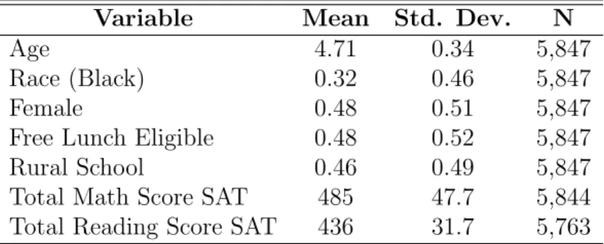
Table 1 presents the summary statistics of the final sample used for the empirical analysis. It consists of 5,781 students who started the project in kindergarten and have valid information on demographic characteristics and test scores. Females constitute 48 percent of the sample, average age at the beginning of 1985 is 4.7 years, 32 percent of the students are black, and 47 percent are eligible for the free/reduced lunch program. Mean years of teacher experience is 9.2, and classes have on average 19 students.

For all the analyses conducted below, the outcome Yics consists of standardized

(to have mean zero and standard deviation one) SAT scores averaged across subjects (math, reading, listening and word study skills), as is common in the literature. The

(35)

policy variablesPcs are class size, teacher experience and proportion of females in the

classroom. In all the models, I include additional control variables Zics accounting

for student gender, race, age and free/reduced lunch status. I start by comparing the results obtained using a standard, linear fixed effects panel data model with the nonparametric estimates of density weighted average derivatives (1.4) and the discrete changes estimators (1.5). Tables 3 to 6 present these results for each policy variable, and for different implementations of the nonparametric series estimators.

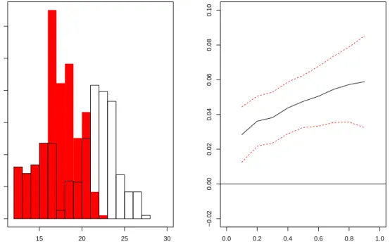
The empirical analysis also includes a counterfactual study of the effect of different policies related to class size, teacher experience and proportion of females in the class-room, using the Counterfactual Distribution function (1.6). Results are presented in Figures 1 to 8. For each figure, the left panel (Panel (a)) displays the original dis-tribution of the policy variable and the resulting counterfactual change. The right one (Panel (b)) reports Quantile Treatment Effects (QTE) for that policy, together with uniformly valid confidence intervals. The QTE estimator measures the impact of the counterfactual policy for quantile q as the difference in outcomes between the

q−th student in the countefactual (treatment) distribution and the q−th student in the original (control) one. For instance, we can compare the median test score for the students in the original distribution and subtract from it the median test score for the students under the counterfactual policy to estimate the effect at the median of the achievement distribution. Note that this estimator will not identify the impact of the policy on a particular student who would have been at the q−th percentile in the absence of the policy. This interpretation is only appropriate if the policy causes no re-ordering of achievement ranks within the distribution. As discussed in Heckman, Smith, and Clements (1997) and more recently in Djebbari and Smith (2008), quantile treatment effects are simply differences between the treatment and control distributions, and recovering quantiles of the treatment effect distribution re-quires specific assumptions about the joint distribution of outcomes in the treatment

(36)

and control states (such as perfect positive or perfect negative dependence). Never-theless, the QTE estimator provides substantial information about treatment effects heterogeneity.

1.4.1 Class Size

Empirical analyses in the STAR Project usually conclude that smaller classes increase student achievement, even after controlling for school fixed effects and teacher characteristics. Table 3 presents estimates of the effect of moving from a class size of 22 to 15 students (the median class sizes for regular and small classrooms in the STAR Project, respectively). In the linear model, this effect is simply βb(22−15),

whereβ is the coefficient associated with class size in the linear model (1.1). Instead, the estimated effect using the discrete changes estimator (1.5) is:

b

∆ (15,22) =

Z b

E(Yics|Pcs = 15, Zics=z, Vs =v)fb_Z_ics_,V_s_|_P_cs(z, v|22)dzdv

− Eb(Y_ics|P_cs = 22)

Using a fixed-effects linear panel data model (Column 1), I find that students benefit about 0.16 standard deviations from assignment to a small class. This is in line with previous findings. However, the nonparametric estimates are actually larger and sta-tistically significant for all the specifications. For example, the effect of assignment to a small class is between 0.3 and 0.43 standard deviations using power series estimators of the regression function. This suggests that unobserved heterogeneity at the school level plays an important role on the impact of class size on student performance. In turn, it could help explain previous findings of different impact estimates for de-mographic groups, as in Schanzenbach (2006). Still, now the effect is more general since unobservable factor are also accounted for. For instance, it is possible that the positive effect of a smaller class size is larger in a school with a better management.

(37)

Next, I extend the analysis by looking atdistributional effects of class size policies using the counterfactual distribution estimator (1.6). The goal here is to see what policies regarding class size would be able to generate the gains in students’ perfor-mance obtained in the previous analysis. I start with a policy that simply reduces class size in the largest classroom (Policy 1):

P_cs∗ =      Pcs if Pcs ≤21 Pcs−5 if Pcs >21

The QTE results are presented in Figure 1.1. The effect is positive throughout the achievement distribution, but heterogeneous, with the biggest impacts among children with scores near the top of the distribution. For example, the test score of a student at the 90th _{percentile in the counterfactual distribution is almost a third}

of a standard deviation higher than the test score of a 90th _{percentile student in the}

original distribution, whereas the difference at the 10th percentile of the distribution are less than a tenth of a standard deviation. These estimates are in line with, although lower in magnitude, the estimates comparing small versus large class sizes in Jackson and Page (2013). High achievers could benefit more from smaller classes if, for instance, teachers in small classes are better able to identify high achievers and use instructional approaches that work well for them.

One potential concern with the previous policy is that it does not take into account feasibility or resource constraints. For example, in order to reduce class size according

to Policy 1, the school would need to hire additional teachers or to enroll some

students in additional classrooms. For this reason, I also look at Policy 2 which keeps the number of students fixed by constructing the counterfactual variable as:

P_cs∗ =      Pcs+ 5 if Pcs ≤21 Pcs−5 if Pcs >21

(38)

From the results in Figure 1.2 we can see that the QTE estimates are close to zero and statistically insignificant over the achievement distribution. This can be explained by the improvements in performance by the students in smaller classes being compen-sated by the worsening in performance by those in larger classes.

Overall, I conclude that the estimated impacts of class size are larger when using a nonseparable model, highlighting the relevance of accounting for heterogeneous treatment effects. The distributional analysis of counterfactual changes also suggests that the impacts are much smaller once we take into account feasibility constrains.

1.4.2 Teacher Experience

Teacher experience has traditionally been an important component of teacher policies in the U.S. school systems. Although recent debates have focused on the development and use of more direct measures of teacher performance (e.g., value-added models, standards-based evaluation), teacher experience continues to play a dominant role in most human resource policies. The underlying assumption is that experience promotes effectiveness and that experience gained over time enhances the knowledge, skills, and productivity of teachers.

Experience is among the most commonly studied teacher characteristic. Several studies find that the impact of experience is strongest during the first few years of teaching: on average, brand-new teachers are less effective than those with some experience (e.g., Rockoff (2004), Rivkin, Hanushek, and Kain (2005), Clotfelter, Ladd, and Vigdor 2007; 2010, Kane, Rockoff, and Staiger (2008), Harris and Sass (2011)), but the greatest productivity gains occur during their first few years on the job, after which their performance tends to level off. Empirical evidence suggests that, on average, students with teachers in their fifth year of teaching score between 5 and 15 percent of a standard deviation higher than students with teachers in their first year on the job (Atteberry, Loeb, and Wyckoff (2013)). There is also evidence that this

(39)

effect is stronger than the effects of teacher licensure tests scores, and even class size (e.g., Clotfelter, Ladd, and Vigdor (2007), Rivkin, Hanushek, and Kain (2005)).

In the STAR Project, Krueger (1999) finds small but positive effects of teacher experience, with a peak at about twenty years: students in classes where the teacher has twenty years of experience tend to score about three percentile points higher than those in classes where the teacher has zero experience, all else being equal. As a whole, however, he concludes that measured teacher characteristics explain relatively little of student achievement on standardized tests. More recently, Chetty, Friedman, Hilger, Saez, Schanzenbach, and Yagan (2011) finds that students randomly assigned to more experienced kindergarten teachers have higher test scores, with the effect being roughly linear. Schanzenbach (2006) analyze the indirect effect of teacher ex-perience by comparing the performance of students in small versus regular class size with teachers of different experience, finding considerable heterogeneity of impacts: students with more experienced teachers show large, stat other observable teacher characteristics such as advanced degrees,istically significant gains from reduced class size. In contrast, students who have a teacher with fewer than five years of experience show smaller and often not statistically significant gains from small classes. Recently, Mueller (2013) finds that this pattern exists at all deciles of the achievement distri-bution, but is less pronounced at lower deciles.

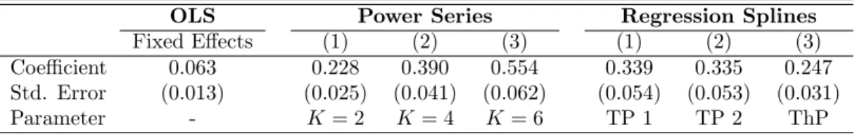
In Tables 4 and 5, I compare the estimates from a linear panel data model (with a quadratic term for the experience variable) to the discrete changes estimator. The goal is to study nonlinear effects of teacher experience on student performance by comparing students with teachers of different years of experience. First, I look at a change from 5 to 10 years of experience (Table 4). Then, I consider a change from 10

(40)

to 15 years in Table 5. Using the nonseparable model (1.2), the effects are:

b

∆ (10,05) =

Z b

E(Yics|Pcs = 10, Zics=z, Vs =v)fb_Z_ics_,V_s|Pcs(z, v|05)dzdv

− Eb(Y_ics|P_cs = 05) b

∆ (15,10) =

Z b

E(Yics|Pcs = 15, Zics=z, Vs =v)fb_Z_ics_,V_s|Pcs(z, v|10)dzdv

− Eb(Y_ics|P_cs = 10)

From Table 4, we can see that the estimate for ∆ (10,05) is around 0.13. That is, students with a teacher with 10 years of experience perform 0.13 standard deviations higher than those with a teacher with only 5 years of experience. We can also see that the point estimates are precisely estimated. This effect is considerably larger than the one obtained using a quadratic model (0.027). Also, in Table 5, changing teacher experience from 10 to 15 years yields a larger impact (between 0.23 and 0.55), which is also larger than the one obtained from a quadratic model (0.063). That is, using the nonseparable model we find evidence of a strong and nonlinear effect of teacher experience. Again, this points to the importance of accounting for unobserved factors in the impact of teacher experience on student performance.

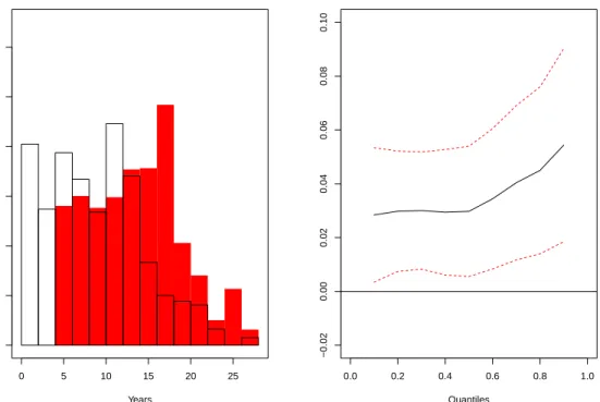
Finally, I look at distributional effects. Policy 1 consists of a general increase of five years in teacher experience,

P_cs∗ =Pcs+ 5

From Figure 1.3, we can see that the effect is positive for all percentiles, but is slightly larger for those at the top quantiles. More importantly, the magnitude of the effect is considerably lower than what is obtained with the discrete changes estimator. To examine whether this could be due to a differential effect coming from teachers of different experience, the next two policies look at the differential effect of teacher

(41)

experience for relatively new versus more experienced teachers. Policy 2 only affects classrooms with less experienced teachers:

P_cs∗ =      Pcs if Pcs >5 Pcs+ 5 if Pcs ≤5

Results are presented in Figure 1.4. The effect of Policy 2 is roughly constant over the achievement distribution. Overall, as with class size, the impacts of these policies are smaller than those obtained with the discrete changes estimators. This could be due to, for example, the impact of teacher experience coming from their interaction with other classrooms characteristics, such as class size (Mueller (2013)).

1.4.3 Proportion of Females

The idea that peers can affect student achievement is based on the assumption that students do not only learn from teachers but also from classmates. For example, students might teach one another by working in groups or having casual discussions, generating knowledge spillovers (see, e.g., Sacerdote (2011) for a review of this liter-ature). One aspect of particular relevance in this context is the gender composition of the classroom. For example, the study of gender peer effects can shed light on the debate single-sex versus coeducational schools (Whitmore (2005)). Gender composi-tion of the classroom could affect student performance in many ways. For example, a higher proportion of girls could improve classroom behavior, reduce classroom disrup-tion and affect the level of violence, creating a better atmosphere for learning (Lavy and Schlosser (2011)). The presence of boys could intimidate girls from speaking up and influence student self-concepts or affect engagement with certain subjects. Fi-nally, classroom composition could also affect the attitude and expectations of teach-ers towards the class, influencing the pace of teaching or their instructional methods (Cunningham and Andrews (1988)).

(42)

Several studies have examined the empirical role of gender composition of the classroom. Hoxby (2000) exploits gender variation in cohort composition in Texas elementary schools and finds that a higher share of girls raises student achievement in math and reading, both for boys and girls. Lavy and Schlosser (2011) find that, in Israeli middle-schools, a 10 percent point increase in the proportion of female students increases girls’ math test scores by 3.7 percent of a standard deviation and boys’ scores by 2.2 percent.

LetPcs be the proportion of females in classroom cin school s. Table 6 compares

the fixed effect estimator of β from model (1.1) to the density weighted average derivative estimator (1.3), for different choices of the series estimator of the derivative of the regression function. We can see that the impacts are considerably larger and statistically significant when we use the nonseparable model.

Next, I look atdistributional impacts. First,Policy 1 implies a 10 percent increase in the proportion of females for all classrooms,

P_cs∗ = (1 + 0.1)×Pcs

From the results in Figure 1.5, we can see that the effect of this policy is positive for all quantiles. There is some heterogeneity (with larger point estimates at the top of the distribution), but with wide confidence intervals. Overall, the impacts are smaller than those obtained in Table 6.

The next policy try to disentangle the mechanism behind the positive effect of the proportion of females on student performance. For example, the effect could be coming from either having more girls in the classroom or more students of the same gender. Then,Policy 2 increases the proportion of females in a classroom with majority of girls, and decreases the proportion in the classrooms with majority of

(43)

boys: P_cs∗ =      (1 + 0.1)×Pcs if Pcs >0.5 (1−0.1)×Pcs if Pcs ≤0.5

From Figure 1.6 we can see that the impacts are now close to zero for all quantiles, suggesting that the effect is actually coming from a larger proportion of females, in line with previous findings in the literature. As with class size, imposing feasibility constraints affects the magnitude of the impacts, suggesting that the implementation of policies regarding gender composition of the classrooms should take into account additional interactions and explore additional channels through which gender peer effects influence student performance.

1.4.4 Tables and graphs

Table 1.1: Summary Statistics - Students

Variable Mean Std. Dev. N

Age 4.71 0.34 5,847

Race (Black) 0.32 0.46 5,847

Female 0.48 0.51 5,847

Free Lunch Eligible 0.48 0.52 5,847

Rural School 0.46 0.49 5,847

Total Math Score SAT 485 47.7 5,844

Total Reading Score SAT 436 31.7 5,763

Table 1.2: Summary Statistics - Classrooms

Variable Mean Std. Dev. N

Teacher Race (Black) 0.16 0.36 302

Teacher has Master Degree 0.36 0.48 302

Teacher Experience (years) 9.32 5.75 302

Class Size 19.4 4.14 302

Note: Original Sample Size: 6325, Sample with non-missing score information: 5907, Sample with non-missing values of class size, teacher experience and gender: 5886. The final sample excludes those with missing values in any of the covariates.