Using the Past to Predict the Present: Confidence Intervals for Regression Equations in Phylogenetic Comparative Methods

Using the Past to Predict the Present: Confidence Intervals

for Regression Equations in Phylogenetic

Comparative Methods

Theodore Garland, Jr.,*and Anthony R. Ives

Department of Zoology, University of Wisconsin, Madison, Wisconsin 53706

Submitted February 4, 1999; Accepted October 6, 1999

abstract: Two phylogenetic comparative methods, independent

contrasts and generalized least squares models, can be used to de-termine the statistical relationship between two or more traits. We show that the two approaches are functionally identical and that either can be used to make statistical inferences about values at internal nodes of a phylogenetic tree (hypothetical ancestors), to estimate relationships between characters, and to predict values for unmeasured species. Regression equations derived from independent contrasts can be placed back onto the original data space, including computation of both confidence intervals and prediction intervals for new observations. Predictions for unmeasured species (including extinct forms) can be made increasingly accurate and precise as the specificity of their placement on a phylogenetic tree increases, which can greatly increase statistical power to detect, for example, deviation of a single species from an allometric prediction. We reexamine pub-lished data for basal metabolic rates (BMR) of birds and show that conventional and phylogenetic allometric equations differ signifi-cantly. In new results, we show that, as compared with nonpasserines, passerines exhibit a lower rate of evolution in both body mass and mass-corrected BMR; passerines also have significantly smaller body masses than their sister clade. These differences may justify separate, clade-specific allometric equations for prediction of avian basal met-abolic rates.

Keywords:allometry, ancestor reconstruction, comparative method, metabolic rate, phylogeny, regression.

Interspecific comparisons have undergone a renaissance in the last decade, and comparative data sets are now analyzed routinely by phylogenetic methods (Eggleton and

*_{To whom correspondence should be addressed; e-mail: tgarland@} facstaff.wisc.edu.

Am. Nat. 2000. Vol. 155, pp. 346–364.q2000 by The University of Chicago.

0003-0147/2000/15503-0005$03.00. All rights reserved.

Vane-Wright 1994; Losos and Miles 1994; Martins 1996a; Garland et al. 1997). Among these methods are several that use phylogenetic information in an explicitly statistical fashion (Grafen 1989; Harvey and Pagel 1991; Garland et al. 1993; Miles and Dunham 1993; Martins and Hansen 1996, 1997; Reynolds and Lee 1996; Schluter et al. 1997; Pagel 1998; Garland et al. 1999). The rationale for these methods is the theoretical prediction and empirical ob-servation that closely related species are more likely to be similar than are distantly related species. Hence, in com-parative studies, species cannot be treated as if they rep-resent independent and identically distributed data points, and ordinary statistical methods, such as standard least squares regression, cannot be used.

The best understood and most prevalent phylogeneti-cally based statistical method is Felsenstein’s (1985) in-dependent contrasts (IC). Inin-dependent contrasts are cal-culated as differences in the value of a trait between two sister species (or internal nodes of a phylogenetic tree) divided by the square root of the sum of their branch lengths (branch lengths must be in units of or proportional to expected variance of character evolution). If evolution along the separate branches of the phylogenetic tree occurs independently, then the contrasts will be statistically in-dependent. Felsenstein’s (1985) original presentation re-lied on a Brownian motion model of character evolution, but the procedure can also be justified on first-principles statistical grounds (Grafen 1989; Pagel 1993). In the con-text of testing for correlated evolution of two characters, simulation studies indicate that independent contrasts are reasonably robust even when character evolution deviates from Brownian motion and when branch lengths used for analyses contain errors, at least if diagnostic tests and transformations of branch lengths are applied (e.g., Type I error rates are not far from what they should be; Grafen 1989; Martins and Garland 1991; Purvis et al. 1994; Dı´az-Uriarte and Garland 1996, 1998; Grafen and Ridley 1996; Martins 1996b; Harvey and Rambaut 1998; Garland and Dı´az-Uriarte 1999). Although Felsenstein’s (1985) original

presentation considered applications to simple linear cor-relation and regression, independent contrasts can also be applied to most problems that require such related statis-tical techniques as principal components analysis, multiple regression, ANOVA, and ANCOVA (e.g., Garland 1992; Garland et al. 1993; McPeek 1995; Dı´az et al. 1996; Gray 1996; Martin and Clobert 1996; Clobert et al. 1998; Bonine and Garland 1999; Foufopoulos and Ives 1999). In addi-tion, by rerooting (see below), the method can be used to estimate trait values and standard errors for internal nodes on a phylogenetic tree (Garland et al. 1999), with results equivalent to those estimated by maximum likelihood (Schluter et al. 1997).

An alternative approach relies on generalized least squares (GLS) models. The phylogenetic information re-quired (topology and branch lengths) is identical to that needed for computing independent contrasts. Rather than constructing contrasts, however, GLS involves regression in which error terms are neither independent nor iden-tically distributed. Instead, the expected variances of and correlations between error terms are assumed to be known from the available phylogenetic topology and branch lengths. Under the assumption of Brownian motion char-acter evolution, GLS estimates of regression parameters are also maximum likelihood estimates, with error terms described by a multivariate normal distribution. Grafen (1989), Martins and Hansen (1997), and Pagel (1998) pro-vide discussions of many possible applications of GLS to comparative analyses, including multiple regression, esti-mating rates of evolution, and reconstructing ancestral traits.

In this article, we address the problem of constructing confidence or prediction intervals for values of a depen-dent variable regressed against an independepen-dent variable. This problem arises frequently in comparative biology, such as in studies of allometry (e.g., Calder 1984; Schmidt-Nielsen 1984; Harvey and Pagel 1991; Garland and Adolph 1994; Garland and Carter 1994; Weathers and Siegel 1995; Reynolds and Lee 1996; Williams 1996; Kozlowski and Weiner 1997; Clobert et al. 1998). As a recent example, Nagy et al. (1999) present a table 2 containing 41 separate allometric equations for predicting field metabolic rates of different clades, habitat, or diet categories. Also in their table can be found the necessary statistics for computing the 95% prediction intervals in the conventional (phylo-genetically uninformed) manner. Nagy et al. (1999, p. 259) note that independent contrasts are an alternative, but then state that independent contrasts do not yield “equations that can be used to predict FMR values directly” and do not yield “statistical parameters that allow calculation of confidence intervals for predicted values.” Both of these claims were correct when their paper was published but

are now obviated by the new methods presented here and implemented in our PDTREE computer program.

To derive formulae for confidence and prediction in-tervals, we use both the IC and GLS approaches. We show that the two approaches produce identical results and can estimate all of the same parameters, including the

Y-intercept in the original data space (contra Pagel 1998, pp. 337, 341). This demonstration is important because many readers of the comparative literature may have been under the impression that IC and GLS represent funda-mentally different ways of analyzing comparative data.

We also present three empirical examples to illustrate the utility and application of these methods. We first show how predictions for unmeasured species can in general be made increasingly accurate and precise as the specificity of their placement on a phylogenetic tree increases. These prediction methods can be used for both extant and extinct (fossil) forms, including putative direct ancestors of extant species (i.e., points along any branch of a phylogenetic tree). Second, we give a specific example in which use of the proposed methods yields greatly increased power to detect whether a particular species deviates from a pre-viously established allometric equation. This example is important not only because it illustrates the increased power that can come from incorporation of phylogenetic information but also because some workers have claimed that independent contrasts could not be used for this pur-pose (e.g., Smith 1994). Finally, we reexamine the allom-etry of avian basal metabolic rate using the data compiled by Reynolds and Lee (1996). This analysis highlights the ability of our methods for mapping phylogenetically cor-rect regressions back onto the original data space to reveal new and striking patterns, such as differences in the rate of evolution of passerines as compared with other birds. The example also shows how, contrary to some previous claims (e.g., Weathers and Siegel 1995), allometric equa-tions derived by conventional and phylogenetic methods can differ significantly, even for a data set that encompasses more than four orders of magnitude in body mass, in-cludes hundreds of species that span almost the full range of phylogenetic diversity in a major clade, and shows a high correlation (r1_0.95).

Statistical Approaches to the Problem of Phylogenetic Correlation

Here we set out the general problem posed by phylogenetic correlation (the tendency for related species to resemble each other) in both the IC and GLS formats. Rather than give a detailed account of these approaches, our intention is to compare them conceptually. Appendices A and B provide the formal statistical derivations of the formulae needed to apply the approaches to data. The IC

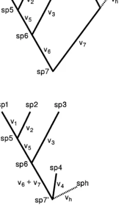
calcula-Figure 1:Phylogenetic relationships for four species (sp1–sp4) with three (sp5–sp7) hypothetical ancestors. Branch lengths ( ) are in units of ex-vi pected variance of character evolution.

tions are implemented in our PDTREE program (available on request from the first author); the GLS approach can be implemented through any commercially available program that manipulates matrices, such as MatLab (MathWorks 1996).

The problem of regression with phylogenetically cor-related data can be stated as follows. Letxiandyi denote the values of an independent and a dependent variable measured for speciesiin a group ofnspecies. Bothxiand yi are assumed to take continuous values. For simplicity, we assume a single independent variable, although our results generalize in a straightforward way to any number of independent variables, including none. With no inde-pendent variables, the analysis corresponds to the case of estimating values of a single trait at internal nodes on a phylogenetic tree (Martins and Hansen 1997; Schluter et al. 1997; Cunningham et al. 1998; Martins and Lamont 1998; Garland et al. 1999). The regression problem can be written as

y =i b01b1xi1ei, (1) where b0 and b1 are regression coefficients and ei is a normally distributed “error” or “residual” term with mean 0. Although this appears to be a standard regression equa-tion, it is not, because values of ei are correlated among different species owing to their shared phylogenetic history.

To illustrate the problem of phylogenetic correlation, consider the phylogeny of four species shown in figure 1. Branch lengths represent the expected variance of char-acter evolution. Thus, species 1 and 2 are more likely to be similar than any other pair of species because they share evolutionary history along branches

v

5 and

v

6, and the variance of the difference between trait values for the two species will be correspondingly low because of the short phylogenetic divergence between them, measured as . Hence, the covariance betweene1ande2(i.e., the

v

11

v

2

portion of the two species’ phenotypes that are not pre-dicted byx) is expected to be high.

Independent-Contrasts Approach

The standard IC approach involves assigning trait values to each of the internal nodes (ancestral species) on the phylogenetic tree. For each internal node, these estimates are a weighted average of the trait values of the two daugh-ter species, with weights proportional to the inverse of the branch lengths between mother and daughter species so that the shorter the branch length, the greater the weight. The independent contrasts are then calculated from the differences between sister taxa throughout the phyloge-netic tree. Except at the root (basal) node (see Garland et

al. 1999), the estimates of ancestral trait values are not optimal estimates; instead, they are merely intermediate steps in the computation of the entire set ofn21 inde-pendent contrasts.

The formulation of regression in terms of independent contrasts removes the constant coefficient b0, making it impossible to map the results from contrasts back onto the original data to obtain confidence intervals for traity

for the tip species. To obtain confidence intervals, the IC approach can be reformulated as

0 0.5

y =i b1(xi2xw)1yw1(

v

i) ei, (2) where yi andxi denote the values of y and x for tip or ancestral species,ywandxwdenote the values at the node directly below speciesi, andeiis normally distributed with mean 0 and variance j2_{. Conceptually, the first term in}

equation (2), b1(xi2xw), describes the dependence ofyi on change in x between the ancestral node w and the present nodei; the second term,yw, incorporates the de-pendence of yion the value of yat the ancestral nodew; and the last term, ₍

_v

0₎0.5_e, accounts for the variance

pro-i i

duced by Brownian motion evolution. Because evolution along sister branches occurs independently, values ofeiare independent of each other. In appendix A, we show how equation (2) can be used to obtain estimates (with stan-dard errors) of confidence intervals for estimates ofyfor each tip species.

The related problem of predicting the value of yfor a new specieshwith known value ofxhis illustrated in figure 2A. The location of specieshon the phylogenetic tree will influence the prediction ofyhbecause (in general) species h will be more similar to closely related species than to distantly related species. The easiest way to obtain pre-diction intervals foryhis to “reroot” the phylogenetic tree,

Figure 2:Illustration of rerooting a phylogenetic tree to predict the value for a hypothetical unmeasured species, designated assph.Ashows that the specieshis putatively the sister of species 4.Bshows the tree rerooted so that the last common ancestor of species 4 andh(sp70) is at the base of the phylogeny. Note that the branch labeledv61v7 is not drawn to scale: it is actually equal to the lengths of the branches, as shown inA.

as is done in figure 2B. In the rerooted tree, specieshis adjacent to the basal node. The estimate (and standard error) of traityat the new basal node,y7, can be obtained

from equation (A13) of appendix A. Because specieshis adjacent to the new basal node, the expected value ofyh equals the estimate ofy7, and the variance of the estimator

ofyhequals the variance ofy7 plus the variance

propor-tional to

v

h that is caused by evolutionary changes from node 7 to species h. The results obtained from this pro-cedure are identical to those that could be obtained via the GLS method of Martins and Hansen (1997; see app. B). To perform these computations in PDTREE, one first reroots the tree; the program will prompt the user for both

andxh.

v

h

Generalized Least Squares Approach

The GLS approach differs from independent contrasts by explicitly dealing with correlations among ei for extant species rather than estimating trait values for ancestral

species. The general regression problem of equation (1) can be written as (Martins and Hansen 1997)

Y=Xb1e, (3) where Y is an n-dimensional vector of values of yi (the measured trait that is considered as a dependent variable),

Xis ann#₂matrix whose first column consists of ones and whose second column contains values xi (the mea-sured trait that is considered as an independent variable), andb= [b0,b1]0(with the prime denoting transpose). Un-der the assumption of Brownian motion evolution,eis an

n-dimensional multivariate normal distribution with mean 0 and variance-covariance matrixj2_{C, wherej}2_{is a scalar}

measuring the overall rate of evolutionary change, as with independent contrasts (matrix j2_{Cis called matrixV by}

Martins and Hansen [1997]). Elements of matrixC(which can be produced with our PDDIST program) describe the phylogenetic relationships as the lengths of the shared branches, from root to last common ancestor, between species (Martins and Hansen 1997; see also box 3 in Cun-ningham et al. 1998). For example, for the tree in figure 1, c =11

v

11

v

51

v

6, and c =12

v

51

v

6. Thus, the greater the shared phylogenetic history between species i and j, the greater the covariance cij. Species 1 and 4 may be considered unrelated; they share no evolutionary history, soc =14 0.

The GLS problem can be analyzed by converting equa-tion (3) into the form of standard linear regression with uncorrelated error terms. Because C is a real symmetric nonsingular matrix, there exists another matrix D such that DCD0=I, the n#_n identity matrix. MatrixD can be used to transform values of traits y and x by letting

, , and . This gives

Z=DY U=DX a=De

Z=Ub1a. (4)

The variance-covariance matrix of a, V{ }, equalsa

E{aa0} =E{De(De)0} =E{Dee0D0} =DE{ee0}D0= (Dj2_C)D0

Thus, no covariance terms appear in the

variance-2

=j I.

covariance matrix ofa, so the error termsai are uncor-related. Furthermore, becauseais a linear transformation of ,e ais normally distributed. Equation (4) can, therefore, be analyzed as a standard least squares regression problem with independent errors (app. B). Unconditional confi-dence intervals for trait y for the extant species are ob-tained by back-transforming fromZto Y. Prediction in-tervals for a new species h can either be calculated by rerooting the phylogenetic tree, as described for the IC method, or by remaining in GLS mode (app. B). This GLS procedure assumes that the elements ofCare known and fixed; more general procedures can be used whenC

con-tains parameters that must be estimated (Judge et al. 1985; Hansen 1997; Martins and Hansen 1997).

Empirical Examples

We provide three empirical examples to illustrate the ferential power of our procedures. All three examples in-volve the allometry of metabolic rate. This theme is chosen because metabolic rate is probably the trait most frequently studied by ecological and comparative physiologists, who in turn are heavy users of the comparative method (Calder 1984; Schmidt-Nielsen 1984; Withers 1992; Garland and Adolph 1994; Garland and Carter 1994; Bradley and Zamer 1999; Garland et al. 1999).

Using Phylogenetic Information to Refine Predictions for Unmeasured Species

We first show how predictions of values for an unmeasured species can be made more precise if the phylogenetic po-sition of the species can be specified (see end of “Inde-pendent-Contrasts Approach”), which can lead to in-creased statistical power (see example in next section). This is important because many workers have complained that phylogenetically based statistical methods only seem to reduce the apparent statistical significance of various effects.

Consider Dutenhoffer and Swanson’s (1996) data on summit metabolic rates of 10 species of passerine birds (fig. 3A). Figure 3Bshows a scatterplot of their data along with a conventional regression line and conventional 95% prediction intervals. Figure 3Cshows the regression line and 95% prediction intervals derived by independent con-trasts, using the methods we have described. These are phylogenetically correct but “generic” prediction intervals, such as those that would be used if one could not specify the phylogenetic position of the hypothetical species to be predicted. In effect, the generic prediction intervals assume that the species to be predicted is attached to the root of the tree and that the branch leading to it ( ) is equal to

v

h the average length of the branches leading from the root to every other tip. Note that these phylogenetically correct but generic prediction intervals are wider than the con-ventional prediction intervals shown in figure 3B.

Figure 3D and 3E shows examples of predicting hy-pothetical extant species whose location on the phyloge-netic tree is known. In both cases, the point estimate for the predicted log10 metabolic rate is closer to the value

(relative to its body mass) of related species. This effect occurs, as it should, because the computations are per-formed by rerooting the phylogenetic tree (as shown in fig. 2) at the node that gives rise to a three-way polytomy comprised of the hypothetical species of interest, its sister

species, and the lineage containing all other species in the data set. The value estimated at this new root node is used to position the regression line vertically in the original data space. Because the value at the new root node will be relatively strongly influenced by the sister species, the elevation of the regression line will move closer to its value for the dependent variable. At the same time, the 95% prediction intervals for particular hypothetical species are considerably narrower than the phylogenetically informed but “generic” prediction intervals shown in figure 3Cand are even narrower than the conventional prediction in-tervals shown in figure 3B. In the limit, if the hypothetical species were attached infinitely close to the sister tip, then the prediction intervals would diminish to 0.

Testing Whether a Single Species Deviates from an Allometric Prediction

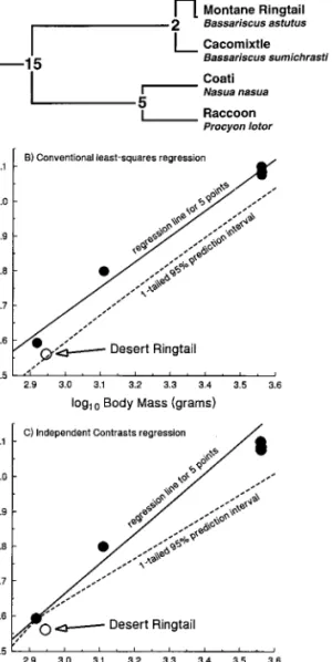
Chevalier (1991) studied metabolism in single populations of four species of procyonid mammals (fig. 4A) and in two separate populations of a fifth species, the ringtail (Bassariscus astutus). A main question of interest was whether the desert population of ringtails had a lower than expected minimal resting metabolic rate in the thermal neutral zone (MRM), which would be expected as an ad-aptation to desert conditions. As discussed in Garland and Adolph (1994), a traditional approach would have been to exclude the datum for the desert ringtail population, use conventional statistics to fit a least squares linear re-gression to the remaining five data points (log trans-formed), compute a one-tailed 95% prediction interval for a new observation, and compare the desert ringtail pop-ulation with this prediction. As shown in figure 4B, the MRM of the desert ringtail population does not fall below the conventional prediction interval, so we would conclude that it does not have a significantly reduced metabolic rate. To repeat the analysis with the methods described above for independent contrasts, the ringtail population is pruned from the tree, the tree is rerooted, and an inde-pendent-contrasts regression line is computed and map-ped back onto the original data space, and the one-tailed 95% prediction interval is computed with PDTREE. As shown in figure 4C, as compared with this phylogenetically informed prediction interval, the desert ringtail does in-deed have a reduced MRM for its body size.

Garland and Adolph (1994, their fig. 4) presented a similar test but remained entirely within the context of phylogenetically independent contrasts. That test yielded similar results but was less intuitive because graphs of contrasts indicate estimates of minimum rates of evolution within particular bifurcations of the phylogeny (differences between sister species or nodes, divided by square roots

Figure 3:A, Phylogenetic relationships of 10 species of birds studied by Dutenhoffer and Swanson (1996), as depicted in their figure 1. Branch length from root (basal node) toContopus virensis 19.7 units. Splits between hypothetical tipsT2andT3and their closest relatives (Parus atricapillus

andContopus virens, respectively) are set at 1.75 units, the same as the split betweenSpizella pusillaandSpizella arborea.B, Log-log plot of summit metabolism in relation to body mass for the birds studied by Dutenhoffer and Swanson (1996; data from their table 1). Least squares linear regression and 95% prediction intervals (dashed lines) are from conventional analysis. C, Same asB, but using phylogenetically independent contrasts, as described in this article and computed in our PDTREE program.D, Predictions (dashed-dotted lines) and 95% prediction intervals (dotted lines) from independent-contrasts procedures, across a range of body masses for hypothetical speciesT2.PaindicatesParus atricapillus, the closest relative ofT2in the data set.E, As inD, but for hypothetical speciesT3.CvindicatesContopus virens, the closest relative ofT3.

Figure 4:Use of new methods presented here to test whether a single species (actually, a desert population of the ringtailBassariscus astutus) deviates from the allometric pattern observed among related species.A, Cladogram (from Decker and Wozencraft’s [1991] cladistic analysis of 129 morphological characters) for the six procyonid taxa studied by Chevalier (1991). Numbers at nodes indicate divergence times in millions of years before present, as estimated from fossil and biogeographic in-formation (corrected from fig. 4 of Garland and Adolph 1994); the two ringtail populations probably began diverging about 10,000 yr ago, at the end of the last ice age.B, Log-log plot of minimal resting metabolism (MRM) versus body mass (from Chevalier 1991; data also shown in Garland and Adolph 1994), along with a conventional least squares linear regression fitted to the five taxa shown as closed circles (slope = 0.734, ) and one-tailed 95% prediction interval for a new

Y-intercept = 0.479

observation. The MRM of the desert population of ringtails does not deviate significantly from this conventional allometric prediction.C, As inB, but regression (slope = 0.864,Y-intercept = 0.071) and one-tailed 95% prediction interval derived by use of methods for phylogenetically independent contrasts presented herein; the desert ringtail population has a MRM that is significantly lower that predicted for its body mass.

of sums of branch lengths) rather than showing actual values for species.

Allometry of Avian Basal Metabolic Rates

Reynolds and Lee (1996) compiled the available data for basal metabolic rates of birds. Phylogenetic relationships (topology and branch lengths, as shown in their figs. A1–A8) for the 254 species were based on Sibley and Ahlquist (1990); the taxonomic scheme in Sibley and Mon-roe (1990) was used to place some species within their respective genera (sometimes along with arbitrary parti-tioning of branch lengths). Reynolds and Lee (1996) checked the adequacy of the branch lengths derived from DNA hybridization (shown in fig. 5A) and used a modified Box-Cox procedure to arrive at an optimal branch length transformation of raising each branch segment to the power20.2 (fig. 5B). Note that this sort of inverse trans-formation actually converts the longest branches into the shortest. Such a transformation is difficult to reconcile with known microevolutionary mechanisms. Therefore, we also report analyses with the original untransformed branch lengths (fig. 5A ) and with all branch lengths set equal to 1. Results do not change very much (see table 1), which is consistent with a number of published em-pirical examples and results of a simulation study that examined the effects of errors in branch lengths (Dı´az-Uriarte and Garland 1998).

For all 254 species, all four of the independent-contrasts regression slopes shown in table 1 exceed the upper 95% confidence interval (0.687) of the conventional estimate. Figure 6 shows the independent-contrasts regression equa-tion presented by Reynolds and Lee (1996, p. 741), based on DNA branch lengths raised to the20.2 power, plotted in the original data space by use of our procedures for computing aY-intercept, confidence interval, and predic-tion interval. The regression line seems to fit the data for nonpasserines fairly well, but it clearly underestimates the log metabolic rate of most passerines in the data set. This is surprising, given that Reynolds and Lee (1996) applied phylogenetic ANCOVA (by both independent contrasts and computer simulation [see Garland et al. 1993]) and found no statistically significant difference between the mass-adjusted log metabolic rates of passerines and non-passerines. What gives?

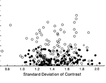
Figure 7 shows a diagnostic plot for contrasts in log10

body mass. The statistical problem illustrated by this plot is the apparently lower average (minimum) rate of evo-lution (Garland 1992) in passerines as compared with other birds in the data set. The mean rank of the absolute values of standardized contrasts in passerines (n =100) is 99.52 as compared with 144.25 for contrasts within the nonpasserines (n =152; Mann-Whitney U =4,902,

two-Figure 5:Topology and branch lengths compiled by Reynolds and Lee (1996, figs. A1–A8) for analyses of avian basal metabolic rate data.A, Branch lengths derived from DNA-hybridization data (from their DATA.PDI file).B, Branch lengths as inAbut transformed by raising each segment to the₂0.2 power, as used by Reynolds and Lee (1996) for independent-contrasts analyses.C, As inBbut with branch lengths within the passerine subclade rescaled so that height from its basal node to highest tip species is 4.0 (see text for explanation).

tailedP!_.0001[the contrast between passerines and their sister clade is excluded from this test]). Moreover, if one examines the absolute values of the residuals from a re-gression of contrasts in BMR on contrasts in mass, the

passerines contrasts (mean rank = 105.84) also average smaller in magnitude than those for other birds (mean

; Mann-Whitney , two-tailed

rank = 140.09 U =5,534 P =

). The differences in rate of evolution are also ap-.0003

parent in figure 2 of Reynolds and Lee (1996): contrasts within passerines are clustered near the origin. Results (not shown) are very similar when all branch lengths are set equal to 1, and the pattern is also apparent with the orig-inal DNA branch lengths.

Thus, relative to DNA branch lengths raised to the20.2 power (or set equal to unity), passerines have a lower rate of log10body mass evolution and also a lower rate of

mass-corrected log10BMR evolution. The overall data set is

com-posed of (at least) two subsets, whose variances differ. Hence, fitting a single regression equation to the entire data set is inappropriate. Several solutions are possible. One would be to fit separate equations to the passerine and nonpasserine data sets. Another is to transform branch lengths differentially (as suggested by Grafen 1989, p. 146) within the passerine clade, which we illustrate.

The result that passerines have a relatively low rate of phenotypic evolution can equally well indicate that they have a high rate of DNA evolution. Indeed, Sibley and Ahlquist (1990), Bleiweiss et al. (1994), and Bleiweiss et al. (1995) have all noted that clades of birds do show significant differences in rates of DNA evolution. In either case, clade-specific variation in rates of evolution can be eliminated by rescaling all branch lengths within one or more clades. We tried several different rescalings of branches within the passerine subclade, using PDTREE, each time rechecking the diagnostic plot shown in figure 7. We found that rescaling the total height of the passerine subclade to 4.0, as shown in figure 5C, yielded absolute values of standardized contrasts that did not differ significantly between passerines (mean rank = 126.31) and nonpasserines (meanrank = 126.63; Mann-Whitney , two-tailed ). For residuals from the

U =7,581 P =.9732

regression of contrasts in log BMR on contrasts in log mass, the passerines contrasts (meanrank = 135.28) also do not differ significantly in magnitude from those for other birds (mean rank = 120.72; Mann-Whitney U =

, two-tailed ).

6,722 P =.1209

Thus, a contrast data set whose variance does not differ significantly between passerines and nonpasserines can be achieved by use of the branch lengths shown in figure 5C. Table 1 shows an allometric equation derived from these branch lengths.

Does Reynolds and Lee’s (1996) conclusion that pas-serines and nonpaspas-serines show no statistically significant difference in mass-corrected basal metabolic rate still hold? Yes. First, we repeated their independent-contrasts analysis (as described on both their p. 739 and fig. 2 [following Garland et al. 1993]) with the rescaled branch lengths

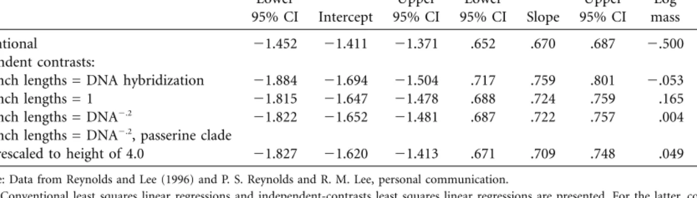
Table 1:Allometric equations for avian basal metabolic rate (log10watts; body mass in log10grams) of all 254 species Intercept Slope Diagnostic correlation Lower 95% CI Intercept Upper 95% CI Lower 95% CI Slope Upper 95% CI Log mass Log BMR Conventional 21.452 21.411 21.371 .652 .670 .687 2.500 2.521 Independent contrasts:

Branch lengths = DNA hybridization 21.884 21.694 21.504 .717 .759 .801 2.053 .165

Branch lengths = 1 21.815 21.647 21.478 .688 .724 .759 .165 .102

Branch lengths = DNA2.2 _{21.822 21.652 21.481 .687 .722 .757 .004 2.034}

Branch lengths = DNA2.2_{, passerine clade}

rescaled to height of 4.0 21.827 21.620 21.413 .671 .709 .748 .049 .051 Source: Data from Reynolds and Lee (1996) and P. S. Reynolds and R. M. Lee, personal communication.

Note: Conventional least squares linear regressions and independent-contrasts least squares linear regressions are presented. For the latter, confidence intervals for theY-intercept are derived by use of the new methods presented herein. For simplicity, these computations use the maximum possible degrees of freedom, as if all of the polytomies (unresolved nodes) in the phylogenetic tree (n =26branches of 0 length) were hard (see Purvis and Garland 1993; Garland and Dı´az-Uriarte 1999). “Diagnostic correlation” is the Pearson product-moment correlation (not through the origin) between the absolute values of standardized independent contrasts and their standard deviations (see text and Garland et al. 1992).

shown in figure 5C. The contrast between passerines and their sister clade was still not a significant outlier (P =

). Repeating the analysis with all branch lengths set .2935

equal yieldedP =.2187. We were concerned, however, that these analyses might be obscured by the inclusion of too wide a range of taxa. Therefore, we pruned the tree of all species except passerines (n =101) and their sister clade (n =85 [Columbiformes 1 Gruiformes1 Charadriifor-mes]). For this reduced data set, examination of diagnostic plots as shown in figure 7 suggested that DNA branch lengths raised to the 0.8 power worked better than those raised to the20.2 power. Again, however, the passerines showed a significantly lower rate of evolution for both log body mass (Mann-Whitney U =2,794, two-tailed P =

) and residual log BMR ( , two-tailed

.0001 U =2,947 P =

). Consequently, we rescaled the branches within the .0005

passerine subclade to a total height of 8.0, which elimi-nated the differences in evolutionary rates. We then re-peated Reynolds and Lee’s (1996) analysis and again found that the contrast between passerines and their sister clade was not a significant outlier (P =.2549).

One interesting additional result of this last analysis was that, for standardized contrasts in log10 body mass, the

contrast between passerines and their sisters was the fifth greatest in magnitude. The probability of this occurring by chance alone is5/185 = 0.0270(this is a two-tailed test because absolute values are analyzed). This result indicates that, on average, the passerines in this data set have sig-nificantly smaller log10body masses than their sister clade

(see Garland et al. 1993, p. 283). We also performed this test for the entire data set of 254 species, using the branch lengths of figure 5C. Here, the contrast between passerines and their sister clade was only the fifty-first most extreme of 253 (P =.2016). Thus, inclusion of all available

spe-cies in the analysis obscures statistically significant clade-specific variation in mean log10body mass.

Discussion

We have shown how to derive both confidence and pre-diction intervals for regression equations derived from in-dependent contrasts but mapped back onto the original data space. The procedures should be of considerable use in comparative studies of allometry, and so forth. They are also useful as a diagnostic in a general sense. For ex-ample, plotting the equation of Reynolds and Lee (1996) back onto the original data space clearly showed that some-thing was amiss (fig. 6).

As explained in Felsenstein’s (1985) original presenta-tion, when independent contrasts are used to estimate the form of a relationship between two traits, including least squares regression, reduced major axis, and major axis slopes (see Garland et al. 1992 for formulae), the line must be forced through the origin. Thus, no estimate of theY -intercept is immediately available. Plotting the estimated slope back onto the original data space would, therefore, be impossible. However, lines describing bivariate re-lationships are generally constructed to pass through the point X Y, . One can, therefore, position a line in the original data space by forcing it through the pointX Y, , where these estimates are computed as the root node es-timate from independent contrasts (see also Garland et al. 1999). The first published example of this procedure is in figure 2 of Garland et al. (1993), which depicts home range areas of mammals in relation to body mass. More recently, Williams (1996) has used the procedure to derive phylo-genetically correct allometric equations for evaporative wa-ter loss of birds. As in many other allometric studies,

Wil-Figure 6:Independent-contrasts regression equation (see table 1) pre-sented by Reynolds and Lee (1996, p. 741), based on DNA branch lengths raised to the20.2 power, plotted in the original data space by use of our new procedures for computing aY-intercept, 95% confidence interval (dotted lines), and 95% prediction interval for a new observation (dashed lines). The regression line seems to fit the data for nonpasserines fairly well (A), but it clearly underestimates the log metabolic rate of most passerines (B) in the data set.

liams (1996) used the equations to predict evaporative water loss values of hypothetical birds of various body sizes. No confidence interval was available for the Y -in-tercept of the regression equation, however, so prediction intervals could not be computed.

Equivalency of the Independent-Contrasts and Generalized Least Squares Approaches

Both independent-contrasts and generalized least squares approaches start from the same statistical model (eq. [1]), use the same phylogenetic information, and give the same results. The main conceptual difference is that IC starts by estimating values of traitsxandyfor ancestral species; the trait value for an ancestral species is the average of its two daughter species weighted by their expected evolu-tionary divergence. GLS, on the other hand, uses a linear transformation of traits x and y in which a new set of variables,ZandU, are created from linear combinations ofYandX, respectively, weighted by matrixD. Thus, both approaches are weighted regression, with their difference being the procedure used to calculate weights.

The conceptual and computational differences between IC and GLS influence how they can be most effectively implemented. In the IC approach, weightings are calcu-lated in terms of trait values of ancestral species. With this interpretation, it is easy to analyze the case in which traits show different rates of evolution (e.g., different branch lengths) across the phylogenetic tree as a whole, or even varying rates within different subsets of the tree (e.g., see fig. 5C). Although in principle these calculations are also possible with the GLS approach, the reference to branch lengths on a phylogenetic tree—rather than a weighting matrix—makes the IC approach more intuitive and vi-sually apparent.

The strength of the GLS approach is that it transforms a regression with correlated residuals into a standard least squares regression problem. This opens the toolbox of familiar statistical diagnostics (such as tests for normality of residuals, homoscedasticity, linearity, etc.) that can be applied with standard least squares regression. Of course, corresponding diagnostics can be applied in the IC ap-proach, which uses regression through the origin, although diagnostics for regression through the origin are less well developed.

Allometry of Avian Basal Metabolic Rate

Table 1 shows that conventional and phylogenetically based estimates of allometric equations can differ signif-icantly, even with large sample sizes (n =254 species), when several orders of magnitude in body mass are in-volved and when the relationship is quite tight

(conven-tional_{r =}2 _0.958). These differences alter one’s conclusions with respect to hypotheses about allometric exponents. Comparative physiologists have argued for years about the theoretical and empirical scaling exponent of basal met-abolic rate. Scaling exponents of both 2/3 and 3/4 are often claimed to have special meaning (references in Calder 1984; Schmidt-Nielsen 1984; Harvey and Pagel 1991; Koz-lowski and Weiner 1997). For the avian metabolic rate

Figure 7:Diagnostic plot of absolute values of standardized independent contrasts in log10body mass versus their standard deviations (square roots

of sums of branch lengths, based on DNA distances raised to the20.2 power, as shown in fig. 5B). This plot suggests that the branch lengths are statistically acceptable in that it shows no overall trend (r =0.004) and approximates one-half of a normal distribution in the vertical di-rection (following Garland et al. 1992). However, it clearly shows that contrasts within the passerines (closed circles) are, on average, smaller in magnitude (Mann-WhitneyU-test, two-tailedP!.0001; a plus sign de-notes the contrast between passerines and nonpasserines, which was ex-cluded from the test). This indicates a difference in the average (mini-mum) rate of evolution (Garland 1992). Thus, the data as a whole are not “identically distributed,” as would be required for subsequent re-gression analyses.

data set taken as a whole, a conventional allometric equa-tion has a slope of 0.670 and a 95% confidence interval that excludes 0.75 (table 1). Independent-contrasts equa-tions have higher slopes, whose lower 95% confidence intervals exclude 0.67. Ironically, our preferred equation for all 254 species (table 1), which incorporates slower evolutionary change within the passerine clade, has a slope of 0.709 and confidence intervals that exclude both 0.67 and 0.75. Before too much is made of these slope estimates and confidence intervals, however, it should be remem-bered that if one attempted to incorporate variance caused by uncertainty about topology, branch lengths or the model of character evolution, then confidence intervals would be even wider (e.g., see Purvis and Garland 1993; Abouheif 1998; Garland and Dı´az-Uriarte 1999).

The conventional and independent-contrasts equations can yield quite different predictions and prediction inter-vals. For a 2-g bird, for example, the conventional equation for all 254 species yields a prediction of 0.0617 w and a 95% prediction interval of 0.0344–0.1105 w; correspond-ing values for the independent-contrasts equation with the

passerine branch lengths rescaled are 0.0392 and 0.0061–0.2544 w. The latter may seem depressingly wide, but they can be narrowed greatly by more precise speci-fication of the phylogenetic position of the species to be predicted, using the new methods that we present here (e.g., see fig. 3 and next section).

We do not offer the allometric equations of table 1 as final answers to problems of scaling avian metabolic rate. Only 2.6% of the world’s extant avian species (9,702 in Monroe and Sibley 1993) are included in the data base. As in Reynolds and Lee’s (1996) original analyses, we have not compared all possible subclades with respect to either allometric relationships or rates of evolution. We suspect that statistically significant heterogeneity of average mass-corrected metabolic rates may yet be shown to exist among clades of birds. For example, three of the four largest out-liers in the nonpasserine data set are hummingbirds, which are only represented herein by four species (of 322 extant). Plus, as noted by Reynolds and Lee (1996), the available data are not a representative sample of birds. This can be illustrated even within the passerines, which consist of two major subclades, oscines (suborder Passeri: 4,580 species) and suboscines (suborder Tyranni: 1,159 species). In this data set, the oscines are represented by 92 species (2.0%), the suboscines by only nine (0.8%). Also, an analysis that accounted for variation associated with diet or ecology as additional independent variables could increase power to detect clade differences. Finally, the topology used for anal-yses includes species grafted onto Sibley and Ahlquist’s (1990) phylogeny with little empirical support, a tree that itself almost certainly contains topological errors (but see Bleiweiss et al. 1994, 1995). As with most broad-scale com-parative studies, both more (and more representative) tip data and additional phylogenetic information would be highly desirable. Ideally, a descriptive and predictive equa-tion for an entire clade, such as Aves, should be derived from a (perhaps stratified) random sampling of its members.

As compared with other birds, we have shown that pas-serines have lower rates of evolution for log body mass (fig. 7), log BMR, and mass-corrected (residual) BMR. These differences were not noted by Reynolds and Lee (1996), in part because they did not have the methods to map regressions with confidence intervals back onto the original data space (e.g., fig. 6). The difference in evolu-tionary rates suggests that separate allometric equations are warranted, even though phylogenetic ANCOVA fails to detect a significant difference in allometric relationships between passerines and nonpasserines (Reynolds and Lee 1996; see also below). The significant difference in mean body mass between passerines (smaller) and their sister clade—reported here for the first time—also bolsters the argument for use of separate equations.

Predictions for Unmeasured Species

Moving beyond the idea of clade-specific allometric equa-tions (see previous section), the new methods presented here allow predictions for unmeasured species to become increasingly precise as phylogenetic information becomes more and more detailed. Consider the question, What is the predicted metabolic rate of a 2-g bird? If the hypo-thetical species is specified no more precisely than “a bird,” then the independent-contrasts equations for all 254 spe-cies would have to be used (and the final one listed in table 1 would be recommended). If it were specified to be a passerine bird, then an equation for the 101 passerine species alone could be used.

If the hypothetical species were specified to be a member of a particular passerine subclade, then the method illus-trated in figure 3 could be used, with the species rooted at the base of the subclade. Alternatively, one could re-compute the independent-contrasts equation using only the data for members of that subclade. The latter proce-dure would be recommended if evidence suggested het-erogeneity in the mass-corrected metabolic rate of different passerine subclades. In general, however, deciding which species to include in a comparative study will often involve trade-offs among sample size, range of the independent variable, and the desire to avoid including apples with citrus (e.g., see discussions in Garland and Adolph 1994; Garland et al. 1997).

If the hypothetical species were specified as the close relative of a particular measured species, then the most precise predictions could be made, in terms of both the point estimate and the width of the prediction intervals. As in most inferential procedures, the more information we have, and the more accurate it is, the better we can

do. Note also that the phylogenetically informed predic-tion intervals (e.g., fig. 3D, 3E) can be narrower than those from conventional analyses (fig. 3B), leading to greatly enhanced statistical power to detect whether a particular species or population deviates from an expectation (e.g., fig. 4). Thus, what phylogeny taketh away (cf. fig. 3Cto fig. 3B), phylogeny giveth back, at least with proper sta-tistical methods.

Paleontologists often estimate body sizes of extinct forms from knowledge of the sizes of one or a few bones (Damuth and MacFadden 1990). With our procedures, the extinct form could be specified in one of three general phylogenetic positions: as a tip on a branch that terminates at some point before the present, as an internal node on the phylogenetic tree, or as a point somewhere along a given branch. The rerooting procedure is used in all three cases. Importantly, the latter two cases involve predictions for hypothetical ancestors that were directly on the line of descent to particular extant species. Previous methods for ancestor reconstruction have been limited to estimation of values at nodes (review in Garland et al. 1999).

Acknowledgments

We thank R. M. Lee III and P. S. Reynolds for providing the metabolic and phylogenetic information (their ASCII file DATA.PDI, dated December 30, 1993); P. E. Midford for computer programming; R. E. Bleiweiss and P. Koteja for helpful discussions; R. Dı´az-Uriarte for comments on an earlier version of the manuscript; and T. F. Hansen and an anonymous reviewer for comments on the submitted versions. T.G. was supported by National Science Foun-dation grants IBN-9157268 and DEB-9509343.

APPENDIX A

Independent-Contrasts Approach

Before deriving statistical properties for the expectation of y given x, it is necessary to review Felsenstein’s (1985) original IC method. Let xi and xj denote values of a trait at two adjacent nodes (or tips)i and j, and let yi andyj denote the values of a second trait that is assumed to depend onx. WithDx = xij i2xjandDy = yij i2yjdenoting the (nonstandardized) contrasts, the regression model of independent contrasts is

0 0

Î

Dy =ij b Dx1 ij1

v

i1

v

jeij, (A1)

where b1 is the slope of the regression, and are the corrected branch lengths below nodesi and j, and eij is a 0 0

v

i

v

j

normal random variable with mean 0 and variancej2_{. The corrected branch length}

_v

0_{takes account of the uncertainty} i

in values estimated for ancestral species. Specifically,

v

0i is calculated recursively from

v

0i=

v

i01(

v v

0 0k l)/(

v

0k1

v

0l), where is the uncorrected branch length and 0 and 0 are the corrected branch lengths above speciesion the phylogenetic

v

i

v

k

v

l

tree. In this particular formulation, the branch lengths for bothxandyare assumed to be the same (Garland et al. 1992; Dı´az-Uriarte and Garland 1996). In general, however, the branch lengths for x andy need not be the same,

which in equation (A1) is equivalent to transformingDyij by multiplying by the ratio

(

Î

v

0i1

v

j0

) (

/

Î

ui01uj0

)

, where

v

i and ui are branch lengths for x and y, respectively. This would be done following any other branch-length transformations.

The estimator ofb1,b1ˆ , is calculated using regression through the origin (Garland et al. 1992), standardizing contrasts by1/

Î

v

0i1

v

0j: 0 0 0 0

Î

Î

O

[

(Dxij)

Z

(

v

i1

v

j

)][

(Dyij)

Z

(

v

i1

v

j

)]

contrasts ˆ b1= ₂ . (A2) 0 0

Î

O

[

(Dxij)

Z

(

v

i1

v

j

)]

contrasts

The estimator of the variance ofeijis

2 ˆ 1 Dyij2b Dx1 ij 2 ˆ j =

O

(

_{0 0}

)

(A3)

Î

N22contrasts

v

1

v

i j

for a phylogenetic tree withNtips (Neter et al. 1989, pp. 167–168). The122a confidence interval forb1ˆ is

2 ˆ j ˆ b15ta,N22 . (A4) 2

Î

O

[

_{(Dx )}

Z

(

Î

_v

0₁

_v

0

)]

ij i j contrasts

The estimate and the confidence interval for the value of yt at tip t depend on the mean E{ytFxt} and variance V{ytFxt} of the distribution ofytgivenxt. The confidence interval is calculated presuming that tiptis rooted directly to the base of the tree with branch length equal to the sum of branch lengths leading to tipt. Formulae forE{ytFxt} andV{ytFxt} are derived below.

For nodes (and tips) other than the basal node, the regression model for independent contrasts can be written

0

Î

y =i b1(xi2xw)1yw1

v

iei, (A5) wherexwandywdenote the values ofxandy at the node immediately preceding node iandei is a normal random variable with mean 0 and variancej2

. The regression model of equation (A5) is formally identical to the model of equation (A1).

The values ofyi at the tips of the phylogenetic tree can be expressed in terms of the basal value ofy (denotedyz) by recursively working down the phylogenetic tree by the relationships

0

Î

y =i b1(xi2xw)1yw1

v

iei 0 0

Î

Î

= b1(xi2xw)1b1(xw2x2w)1y2w1

v

iei1

v

wew _ (A6) 0

Î

= b1(xi2xz)1yz1

O

v

kek, lineage

where the subscript 2wdenotes the node two below nodei, and the summation is taken over all nodeskin the lineage between node i and the basal node. Incidentally, this formula demonstrates the need for the independent-contrasts method. The value ofyidepends on the values ofekalong the lineage from the basal node. For tips that partially share a lineage, values ofyishare some of the same values of ek, making them nonindependent.

ˆ

ˆ ˆ

y =i b1(xi2xw)1yw, (A7) whereb1ˆ is given by equation (A2). The estimator of the basal node is derived using the usual independent-contrasts method (Felsenstein 1985; Garland et al. 1999):

0_ˆ 0_ˆ

v

2y11

v

1y2

ˆ

y =z

_v

0 ₁

_v

0 , (A8)

1 2

whereyˆ1andˆy2are the estimates of values ofyat nodes 1 and 2 above the basal node, which themselves are obtained recursively from the preceding nodes by use of the formula

0_ˆ 0_ˆ

v

jyi1

v

iyj

ˆ

y =k

_v

0₁

_v

0 . (A9)

i j

The value ofxat the basal node,xz, is calculated similarly.

For tipt, the random variableyˆtis normally distributed because it is the sum of normal random variables bˆ1and . The expectation of givenxtis

ˆ ˆ yi yt ˆ ˆ ˆ E{yF_{x}= E{b(x} 2_{x )}1_{y }} t t 1 t w w ˆ _ˆ = E{b1(xt2xz)1yz} (A10) = b1(xt2xz)1yz, and its variance is

ˆ ˆ ˆ V{yF_{x}= V{b(x} 2_{x )}1_{y }} t t 1 t w w ˆ _ˆ = V{b1(xt2xz)1yz} 2 ˆ _ˆ = V{b1}(xt2xz) 1V{yz} (A11) 0 0 2 (xt2xz) 2

v v

1 2 2 = j 1 _{0 0}j . 2

v

1

v

1 2 0 0

Î

O

[

(Dxij)

Z

(

v

i1

v

j

)]

contrasts

In equation (A11), the expression forV{bˆ1}derives from equation (A2). From equation (A8), the value ofV{yˆz}is obtained from 2 2 0 0 0 0

v

2 0 2

v

1 0 2

v v

1 2 2 ˆ V{yz}=

(

_v

0₁

_v

0

)

v

1j 1

(

_v

0₁

_v

0

)

v

2j =

_v

0 ₁

_v

0j . 1 2 1 2 1 2

Finally, independence of_bˆ1andyˆi follows from Fisher’s lemma in a manner analogous to standard linear regression (Larsen and Marx 1981).

From regression through the origin, _ˆ2 2 is a 2 distribution. From equations (A10) and (A11), [(N22)j]/j xN22 ˆ ˆ yt2[b1(xt2xz)1yz] 2 (xt2xz) _{0 0 0 0} j

Î

O

_[( Î0 0 2 1[(

v v

1 2)/(

v

11

v

2)] Dxij) (

Z

v1i vj)] contrasts

is normally distributed with mean 0 and variance 1. Therefore, ˆ ˆ yt2[b1(xt2xz)1yz] (A12) 2 0 0 0 0 0 0 2 2

Î

_jˆ

(

(xt2xz)

Z

{

O

[

(Dxij)

Z

(

Î

v

i1

v

j)

]

}

1[(

v v

1 2)/(

v

11

v

2)]

)

contrasts

is a StudenttN22distribution, and the122a confidence interval forE{yˆtFxt} is

ˆ ˆ yz1b1(xt2xz) 2 2 0 0 ˆ 1 Dyij2b Dx1 ij 2 Dxij

v v

1 2

Î

5ta,N22

O

(

_{0 0}

)

{

(xt2xz)

Z

[

O

( )

_{0 0}

]

1 0 0

}

. (A13) contrasts

Î

contrasts

Î

N22

v

_i1

v

_j

v

_i1

v

_j

v

11

v

2

Equation (A13) leads directly to the confidence interval for they-intercept of the independent-contrasts regression by settingx =t 0.

To obtain an estimate and prediction interval ofyhfor a new speciesh, first suppose that specieshis rooted to the base of the phylogenetic tree on a branch of length

v

h. Then the model for the estimator ofyhis

ˆ

ˆ ˆ

y =h b1(xh2xw)1yw1

v

heh, (A14)

whereehis a normally distributed random variable with mean 0 and variance j

2_{. Following from the derivation of}

equation (A13), the prediction interval foryˆhis

ˆ ˆ yh1b1(xh2xz) 2 2 0 0 ˆ 1 Dyij2b Dx1 ij 2 Dxij

v v

1 2

Î

5ta,N22

O

(

_{0 0}

)

{

(xh2xz)

[

O

( )

_{0 0}

]

1 0 0 1

v

h

}

. (A15) contrasts

Î

contrasts

Î

N22

v

_i1

v

_j

U

v

_i1

v

_j

v

11

v

2

To obtain prediction estimates ofyˆhwhen species his not rooted to the base of the tree, the tree can be rerooted as illustrated in figure 2B and the analysis performed as described above. The actual selection of the branch length depends on the application. If is known for a particular species, then it can be used in equation (A15). For the

v

h

v

h

prediction interval for a species whose location on the phylogenetic tree is unknown, the species could be rooted to the base of the tree, and

v

hcould be given the average base-to-tip distance for all known species in the phylogeny. PDTREE calculates the estimates of_bˆ (eq. [A2]),_jˆ2(eq. [A3]), confidence intervals for_ˆy (eq. [A13]), and predictions

1 i

for species rooted to the base of the phylogenetic tree (eq. [A15]). PDTREE can also reroot the phylogenetic tree,

ˆ

yh

thus allowing computation of prediction intervals for hypothetical new species anywhere. APPENDIX B

Generalized Least Squares Approach

Rather than restrict the analysis to a single independent variable, we will considerPindependent variables. Thus, let

Xbe then#Pmatrix with elementsxik, wherei =1, ),ndenotes the species, andk =1, ),Pdenotes the independent variable. To include a constant (intercept), the first independent variable is given the value of 1 for all species. The regression problem can be written

Y=Xb1e, (B1) where the vectors Y= [y1,y2,),yn]0, e= [e1,e2,),en]0, and b= [b1,b2,),bP]0. Following Martins and Hansen (1997), letj2_{Cbe the variance-covariance matrix ofe;j}2_C=E{ee0_{}. (Note that Martins and Hansen [1997] denote}

our matrixj2_{CasV.) Thei}2_jth_{element ofCis the sum of branch segment lengths that speciesiand speciesjshare}

in common. The total branch lengths from root to tips are not constrained to be the same for all species.

As described in the text, let D be an n#_n matrix such that _DCD0_=I. Obtaining D involves singular value decomposition ofC, which is performed by statistical packages such as MatLab with the SVD() function. Transforming variables as Z=DY,U=DX, and a=Deconverts the GLS problem given by equation (B1) into a standard least squares problem given by equation (4). Statistical inference can be performed forZand then back-transformed toY. Below is a set of standard formulae (Judge et al. 1985; Neter et al. 1989): estimate of , :b bˆ

0 21 0 0 21 21 0 21

ˆ

b= (U U) (U Z) = (X C X) (X C Y); (B2)

unbiased estimate of variancej2_,jˆ2_:

2 ˆ 0 ˆ ˆ 0 21 ˆ ˆ j = (Z2Ub) (Z2Ub)/(n2P)=(Y2Xb)C (Y2Xb)/(n2P); (B3) variance-covariance matrix of ,b V{ }:b 2 0 21 2 0 21 21 V{b}=j (U U) =j (X C X) ; (B4)

estimated variance-covariance matrix ofb, s2_{b}:

2 _ˆ2 0 21 _ˆ2 0 21 21

s {b} =j(U U) =j(X C X) ; (B5)

estimates of mean responses ofY,Yˆ:

21 ˆ

ˆ

Y=D (DXb); (B6)

estimated variance-covariance matrix of mean responses ofY, s2_{{ }:Y}ˆ 2 ˆ 21 2 ˆ 210 2 0

s {Y} =D s {Z}(D ) =Xs {b}X. (B7)

Note that with the variance-covariance of mean responses, s2_{{ }, it is possible to calculate the joint confidence intervalsY}ˆ

for the mean responses .Yˆ

These formulae are exact under the assumption of Brownian motion evolution and can be used for statistical inference in the usual least squares regression fashion. Thus, n /j2

follows ax2

distribution with degrees of

2

ˆ

j n2P

freedom. Similarly,(bk2bˆk)/s{bˆk}and(y2yˆi)/s{yˆ}followt-distributions withn2Pdegrees of freedom. Even though these expression are exact only under Brownian motion evolution, by the Central Limit Theorem they are asymptotically correct for large sample sizes when error terms are nonnormal, provided the errors are identically distributed and have covariance structure given by C. The general expression for the (nonestimated) variance-covariance matrix, , can be used to analyze cases in whichCis unknown; this is the case discussed broadly by Martins and

2 0 21 21 j (X C X)

Hansen (1997, pp. 659–662) and explains the difference between their discussion and the estimation procedure presented here. Note also that the estimates and standard errors forb0 andb1given in figure 2 of Martins and Hansen (1997)

are incorrect because of a computational error (T. F. Hansen, personal communication).

It is instructive to compare these results with those obtained from independent contrasts in appendix A. For the case of only one independent variable, the following identities hold: estimate of variancej2_,jˆ2_:

2 ˆ 0 ˆ ˆ j = (Z2Ub) (Z2Ub)/(n22) 2 ˆ 1 Dyij2b Dx1 ij =

O

(

_{0 0}

)

; (B8)

Î

N22contrasts

v

1

v

i j

estimated unconditional variances ofY, diag(s2

{ }):Yˆ

2 ˆ 2 0 _ˆ2 0 21 21 0

diag(s {Y}) = diag(Xs {b}X) =jdiag[X(X C X) X)]

2 0 0 0 0 0 0 2 2

Î

ˆ = j

({

(xt2xz)

Z

[

O

(Dxij)

Z

(

v

i1

v

j

)

]}

1[(

v v

1 2)/(

v

11

v

2)] .

)

(B9) contrasts

This last expression leads to the further identity that

0 0

v v

1 2 0 21 21

(1 C 1) = _{0 0}, (B10)

v

11

v

2

where1 is an n#₁ vector of ones. These expressions show the clear relationships between weightings in terms of in the IC approach and weightings in terms ofCin the GLS approach.

0

v

i

Prediction intervals for a new specieshcan either be calculated by rerooting the tree, as described for the IC method, or by explicitly calculating the conditional mean and variance of the error termehfor the new species. For new species h, the value ofyhis given by

y =h b01b1xh1eh, (B11)

whereehis normally distributed with mean mand variancej 2 _c

h. Bothm andchdepend on the error terms obtained for all related species on the phylogenetic tree (here, “related” means that the amount of shared branch length is1_0).

In particular, ifcihgives the sum of branch lengths shared by speciesiandh, andCihis then#1 vector of values of

cihfor all speciesi other thanh, then 0 2 , and (Box et al. 1994, pp. 282–285; see

1 _¯ 0 21

m=C Cih (X2x) c = ch hh2C C Cih ih

also Martins and Hansen 1997, p. 661). The computations used in appendix B are not performed by PDTREE, but they can be performed using such software packages as MatLab (MathWorks 1996).

Literature Cited

Abouheif, E. 1998. Random trees and the comparative method: a cautionary tale. Evolution 52:1197–1204. Bleiweiss, R., J. A. W. Kirsch, and F. J. Lapointe. 1994.

DNA-DNA hybridization-based phylogeny for “higher” nonpasserines: reevaluating a key portion of the avian family tree. Molecular Phylogenetics and Evolution 3: 248–255.

Bleiweiss, R., J. A. W. Kirsch, and N. Shafi. 1995. Confir-mation of a portion of the Sibley-Ahlquist “tapestry.” Auk 112:87–97.

Bonine, K. E., and T. Garland, Jr. 1999. Sprint performance of phrynosomatid lizards, measured on a high-speed treadmill, correlates with hindlimb length. Journal of Zoology (London) 248:255–265.

Box, G. E. P., G. M. Jenkins, and G. C. Reinsel. 1994. Time series analysis: forecasting and control. Prentice Hall, Englewood Cliffs, N.J.

Bradley, T. J., and W. E. Zamer. 1999. Introduction to the symposium: what is evolutionary physiology? American Zoologist 39:321–322.

Calder, W. A. 1984. Size, function and life history. Harvard University Press, Cambridge, Mass.

Chevalier, C. D. 1991. Aspects of thermoregulation and energetics in the Procyonidae (Mammalia: Carnivora). Ph.D. diss. University of California, Irvine. 202 pp. Clobert, J., T. Garland, Jr., and R. Barbault. 1998. The

evolution of demographic tactics in lizards: a test of some hypotheses concerning life history evolution. Journal of Evolutionary Biology 11:329–364.

Cunningham, C. W., K. E. Omland, and T. H. Oakley. 1998. Reconstructing ancestral character states: a critical reappraisal. Trends in Ecology & Evolution 13:361–366. Damuth, J., and B. J. MacFadden, eds. 1990. Body size in mammalian paleobiology: estimation and biological im-plications. Cambridge University Press, New York. Decker, D. M., and W. C. Wozencraft. 1991. Phylogenetic