Mapping microarray gene expression data into dissimilarity spaces for tumor classification

(1)

Mapping microarray gene expression data into

dissimilarity spaces for tumor classification

Vicente Garc´ıaa, J. Salvador S´anchezb,∗

a_{Department of Electrical and Computer Engineering, Instituto de Ingenier´ıa y}

Tecnolog´ıa, Universidad Autónoma de Ciudad Juárez, Av. del Charro 450 Norte, 32310 Ciudad Juárez, Chihuahua, Mexico

b_{Institute of New Imaging Technologies, Department of Computer Languages and}

Systems, Universitat Jaume I, Av. Sos Baynat, s/n, 12071 Castell´o de la Plana, Spain

Abstract

Microarray gene expression data sets usually contain a large number of genes, but a small number of samples. In this article, we present a two-stage classification model by combining feature selection with the dissimilarity-based representation paradigm. In the preprocessing stage, the ReliefF al-gorithm is used to generate a subset with a number of top-ranked genes; in the learning/classification stage, the samples represented by the previously selected genes are mapped into a dissimilarity space, which is then used to construct a classifier capable of separating the classes more easily than a feature-based model. The ultimate aim of this paper is not to find the best subset of genes, but to analyze the performance of the dissimilarity-based models by means of a comprehensive collection of experiments for the clas-sification of microarray gene expression data. To this end, we compare the classification results of an artificial neural network, a support vector machine

∗_{Tel.: +34 964 728350, Fax: +34 964 728730}

Email addresses: vgarciaj@gmail.com(Vicente Garc´ıa),sanchez@uji.es(J. Salvador S´anchez)

(2)

and the Fisher’s linear discriminant classifier built on the feature (gene) space with those on the dissimilarity space when varying the number of genes se-lected by ReliefF, using eight different microarray databases. The results show that the dissimilarity-based classifiers systematically outperform the feature-based models. In addition, classification through the proposed rep-resentation appears to be more robust (i.e. less sensitive to the number of genes) than that with the conventional feature-based representation.

Keywords: Gene expression, Dissimilarity space, Feature selection, Classification.

1. Introduction

Microarray biotechnology is able to record and monitor the expression levels of thousands of genes simultaneously within a few different samples, which has led to a growing interest for its application to a broad variety of biological and biomedical problems. Microarray gene expression data has extensively been applied to distinguish between cancerous and normal tissues,

to classify different types or subtypes of tumors, and also to predict the response to a particular therapeutic drug and the risk of relapse [2, 22, 30, 40]. In the literature, one can find a plethora of machine learning models that have been used for microarray gene expression analysis and prediction, such as support vector machines, K nearest neighbors, decision trees, Bayesian models, artificial neural networks, and classifier ensembles [3, 11, 15, 25, 32, 42]. A review of computational intelligence techniques applied to various biomedical problems can be found in the paper by Hassanien et al. [14]. All these methods have been defined to be used in a feature space, but other

(3)

alternative spaces, which have been reported to be truly effective on a number of real-life problems, could also beexploited for biomedical applications. One of these alternatives is the dissimilarity space, which constitutes the target of the present work.

In the dissimilarity-based classification paradigm [26], samples to be clas-sified are encoded using pairwise dissimilarities (distances from other samples in the data set). The justification for constructing classifiers in a dissimilarity space is that a dissimilarity measure should be small for similar samples and large for distinct samples, thus allowing for efficient and reliable discrimina-tion of classes. Another important characteristic is that the dimensions of a dissimilarity space symbolize homogeneous types of information and there-foreall dimensions can be considered as equally relevant. On the other hand, for a complex problem, a simple linear classification model in a dissimilarity space could separate the classes more easily than the same classifier in a feature space [29]. The dissimilarity-based approach has been applied suc-cessfullyto many fields, such as computer vision, medical imaging and remote sensing [35, 38] but, to the best of our knowledge, not yet to biomedicine.

However, classification using microarray data poses a major computa-tional challenge due to the very high number of genes (G) and the low number of samples (n) [10]. Typically, the number of genes is of the or-der of thousands while the number of samples is less than a hundred. This phenomenon is referred to as the ‘large G, smalln’ or ‘curse of dimensional-ity’ problem in statistics,which increases the complexity of the classification task considerably, degrades the generalization ability of classifiers and hin-ders the understanding of the relationships among the genes and the tissue

(4)

samples [9, 31]. The common practice to tackle this problem is using some form of feature (gene) selection as a preprocessing step to be applied be-fore building the classifier. Gene selection allows the removal of irrelevant, noisy and redundant genes from microarray data, thus preserving the genes thatbest discriminate biological samples of different types (tissue categories, disease states or clinical outcomes).

Among the most successful gene selection methods are those based on gene ranking or scoring [17, 20, 34, 41]. In this case, each gene is evaluated individually and assigned a score reflecting its correspondence with the class according to certain predetermined criteria. Afterwards, genes are ranked

by their scores and a number of the top-ranked ones, which can be deemed as the most informative genes, are chosen. In practice, the gene ranking algorithms are filters that compute some measure to determine how much more significant each gene is than the others [13]. Some well-established score-based methods include the t-test, the non-parametric Kruskal-Wallis statistic, the Welch test statistic, information-theoretic measures, Kendall’s correlation coefficient, χ2_{-statistic and ReliefF, among others.}

In the present study, we propose a method to classify the microarray data using a dissimilarity space together with the selection of a number of top-ranked genes through the ReliefF algorithm. Here we have adopted the ReliefF algorithm because of its simplicity and good performance in microar-ray data analysis [5, 39], but other methods could be applied as well [6, 36]. Hence, instead of working with genes directly, the samples are defined by pairwise dissimilarity vectors because our hypothesis is that the samplesthat

(5)

re-lated to the problem under study. We are, then, investigating the feasibility and efficiency of the new method by comparing the performance of models built both on dissimilarity and feature spaces using an artificial neural net-work, the Fisher’s linear discriminant and a support vector machine for the classification of eight benchmarking microarray gene expression databases. Note that our purpose here is not to find the best subset of genes or the best performing classifier, but we are trying to gain some insight into the perfor-mance of the dissimilarity-based classification models applied to microarray gene expression data.

The rest of this article is organized as follows. Section 2 presents the details of the two-stage method proposed here, including a description of the ReliefF algorithm and the bases of the dissimilarity-based classification approach. The experimental databases and set-up are given in Section 3. Section 4 discuss the results. Finally, Section 5 summarizes the most inter-esting conclusions drawn from this study and provides possible directions for future research.

2. Methods

In this section, we provide a description of the two methods that com-prise the procedure for classification of microarray gene expression data: the ReliefF algorithm for gene selection and the dissimilarity space approach to classification. A general overview of the complete process for both building the model and classifying the test samples is also included.

(6)

2.1. Gene selection with ReliefF

ReliefF is an improved version of the Relief procedure to estimate the quality of features in problems with strong dependencies between features [18, 33]. The basic idea of the ReliefF algorithm lies on adjusting the weights of a vector W = [w(1), w(2), . . . , w(G)] to give more relevance to features that better discriminate the samples from neighbors of different class.

It randomly picks out a samplexand searches forK nearest neighbors of the same class (hits, hj) and K nearest neighbors from each of the different

classes (misses, mj). If x and hj have different values on gene f, then the

weight w(f) is decreased because it is interpreted as a bad property of this gene. In contrast, ifxand mj have different values on the gene f, then w(f)

is increased. The whole process is repeated t times, updating the values of the weight vector W as follows

w(f) = w(f)− ∑K j=1dist(f, x, hj) t·K (1) + ∑ c̸=class(x) P(c) 1−P(class(x))· ∑K j=1dist(f, x, mj) t·K

where P(c) is the prior probability of class c,P(class(x)) denotes the prob-ability for the class of x, and dist(f, x, mj) represents the absolute distance

between samples xand mj in the gene f.

The algorithm assigns negative values to genes that are completely irrel-evant and the highest scores for the most informative genes. In general, one will then select the g top-ranked features in order to build the classifier with a presumably much smaller subset of genes (g ≪G).

(7)

2.2. Classification in the dissimilarity space

Traditional learning and classification methods rely on the description of samples by means of set of observable features. An alternative to the fea-ture space is the dissimilarity space proposed by P¸ekalska and Duin [26], in which the dimensions are defined by vectors measuring pairwise dissimilari-ties between examples and individual prototypes from an initial representa-tion set R = {p1, . . . , pr}. This can be chosen as the complete training set

T ={x1, . . . , xn}, a set of generated prototypes, a subset of T that covers all

classes, or even an arbitrary set of labeled or unlabeled samples [28].

Given a dissimilarity measured(·,·), which is required to be nonnegative and to obey the reflexive condition (d(xi, xi) = 0) but it might be non-metric,

a dissimilarity representation is defined as a data-dependent mapping func-tionD(·, R) fromT to the dissimilarity space. This means that every example xi ∈ T is represented by an r-dimensional vector in the dissimilarity space,

D(xi, R) = {d(xi, p1), . . . , d(xi, pr)}, that is, each dimension corresponds to

a dissimilarity to a prototype from R. Therefore, dissimilarities between all examples in T toR are represented by a matrixD(T, R) of sizen×r, which corresponds to the dissimilarity representation we want to learn from [27].

D(T, R) =         d(x1, p1) d(x1, p2) · · · d(x1, pr) d(x2, p1) d(x2, p2) · · · d(x2, pr) .. . ... . .. ... d(xn, p1) d(xn, p2) · · · d(xn, pr)        

In a general classification scenario, a drawback related to the use of fea-tures is that different samples may have the same representation, thus result-ing in class overlap (i.e. some samples of different classes are represented by

(8)

the same feature vectors). In the dissimilarity space, however, only identical samples (with the same class label) have a zero-distance, which means that there does not exist class overlap.

2.3. General overview of the process

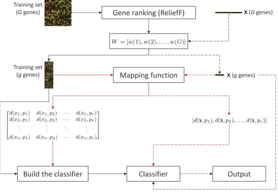
The method proposed in this article combines the ReliefF algorithm for gene selection with the dissimilarity-based representation for classification of microarray gene expression data. The flowchart of the complete learn-ing/classification procedure is shown in Fig. 1.

Gene ranking (ReliefF)

Mapping function

Build the classifier

Training set (G genes) Training set (g genes) Classifier Output X (G genes) X ₍g genes)

Figure 1: Flowchart of the proposed learning and classification methodology (red lines correspond to the stage for building the dissimilarity space).

(9)

the ReliefF algorithm to the data set containing G genes and n samples, whose output is a weight vector W that allows to select a subset with the

g top-ranked genes. Next, the resulting data set with the selected genes is mapped into a dissimilarity space represented by a matrix of size n ×r (here we will take r to be equal to n). Finally, the classifier is built in the dissimilarity space just defined.

In the testing phase (dashed lines), when a new instancexhas to be clas-sified, its dimensionality is firstly reduced according to the subset of g genes selected in the training phase. Then the sample is mapped into the dissim-ilarity space by calculating the dissimdissim-ilarity between x and all prototypes in the representation set R, resulting in a one-dimensional matrix (vector) D(x, R) = [d(x, p1), d(x, p2), . . . , d(x, pr)]. This dissimilarity vector D(x, R)

is passed through the classifier for yielding a class label to the new instance

x.

3. Experiments

To analyze the performance of the method, we have conducted a series of experiments on a collection of data sets available at Kent Ridge Biomedi-cal Data Set Repository (http://datam.i2r.a-star.edu.sg/datasets/krbd). Ta-ble 1 provides a brief description of each data set, including the number of genes, the number of samples and the size of each class.

The experiments have consisted of studying the classification performance on the feature and dissimilarity spaces when varying the number of genes selected by ReliefF from 1 to 150. Bearing in mind that the aim of this study is to compare both representations, not to find the optimal number

(10)

Table 1: Characteristics of the microarray data sets.

Genes Samples Class1/Class2

Breast 24481 97 Relapse (46)/Non-relapse (51)

CNS 7129 60 Failure (39)/Survivor (21)

Colon 2000 62 Tumor (40)/Normal (22)

DLBCL-Stanford 4026 47 Germinal (24)/Activated (23)

Lung-Brigham 12533 181 MPM (31)/ADCA (150)

Lung-Michigan 7129 96 Tumor (86)/Normal (10)

Prostate 12600 136 Tumor (77)/Normal (59)

Ovarian 15154 253 Cancer (162)/Normal (91)

of genes, the experiments have been confined to the 150 top-ranked genes because it has been observed that when the number of genes is greater than 150, the variation in accuracy is not significant [21, 24, 37]. Although one might achieve better results selecting a different number of genes for each database, these improvements would apply equally to both representations; hence, for the purpose of this paper, the key question is not how many genes should be selected to perform the best with each database. Moreover, it is important to remark that the behavior of the optimal number of genes relative to the sample size also depends on the classifier [16].

3.1. Experimental design

We have focused our study on three linear classification models, the Fisher’s linear discriminant (FLD), the support vector machine (SVM) and the multilayer perceptron neural network (MLP) comparing their behavior on the feature space and on the dissimilarity space after selecting a number of top-ranked genes with the ReliefF algorithm. Therefore, combining the classifiers and the representations, we have six different approaches: (i) FLD

(11)

on the feature space (FLD-F), (ii) FLD on the dissimilarity space (FLD-D), (iii) SVM on the feature space (SVM-F), (iv) SVM on the dissimilarity space (SVM-D), (v) MLP on the feature space (MLP-F), and (vi) MLP on the dissimilarity space (MLP-D).

The parameter settings for the algorithms used in the experiments are as follows. The number of nearest neighbors K for the ReliefF algorithm has been set to 1 due to the small size of the data sets. The MLP neural networks have used a sigmoidal transfer function and the backpropagation learning algorithm. The SVM models have been constructed using a linear kernel function, which has been regarded as one of the best options in many bioinformatics applications [1], with the soft-margin constant C = 1.0. On the other hand, due to the small size of the training data sets, we have chosen the representation set R to be equal to the training set T (that is, r = n), which means that the mapping function from T to the dissimilarity space results in a square matrix of size n×n.

The 10-fold cross-validation method has been adopted for the experimen-tal design because it seems to be the best estimator of classification perfor-mance compared to other methods, such as bootstrap with a high computa-tional cost or re-substitution with a biased behavior [4]. Each original data set has randomly been divided into ten stratified parts of equal (or approxi-mately equal) size; for each fold, nine blocks have been pooled as the training set, and the remaining part has been used as an independent test set.

3.2. Performance evaluation metrics

In most biomedical applications, it is important to assess not only the accuracy of the model, but also false-positive and false-negative errors (or

(12)

their counterpart, the true-negative and true-positive hits respectively) be-cause they usually have asymmetric costs [19, 23]. Hence, the performance of the methods has been analyzed by means of three metrics that can be easily

computed from a 2×2 confusion matrix as that shown in Table 2, where

each entry (i, j) contains the number of correct/incorrect predictions: • Accuracy: Acc= (T P +T N)/(T P +F N +T N +F P)

• True-positive rate, which is the proportion of positive samples that are correctly classified: T P r =T P/(T P +F N)

• True-negative rate, which is the proportion of negative cases that are correctly classified: T N r=T N/(T N+F P)

where T P and T N denote the number of positive and negative examples

correctly classified respectively, whereas F P and F N represent the number of misclassifications on negative and positive examples respectively1_.

Table 2: Confusion matrix.

Actual class

Positive Negative

Predicted class Positive T P F P

Negative F N T N

1_{Note that we have considered that the samples from class1 shape the positive class}

(13)

4. Results

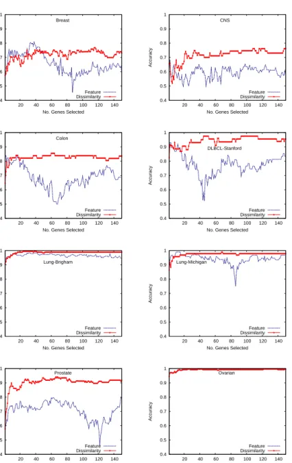
For each database, we have first compared the average classification accu-racies of FLD (Fig. 2), SVM (Fig. 3) and MLP (Fig. 4) on the feature space (blue line) with those on the dissimilarity space (red line) when using the different subsets of genes. One can observe that in general, the performance of classifiers built from the dissimilarity space is superior to that of the mod-els constructed from the feature space, especially in the case of FLD. It is also important to note that when varying the number of genes selected, the accuracy seems to keep more steady using the classifiers on the dissimilarity space than on the feature space. This suggests that the dissimilarity-based models are less sensitive not only to the amount of genes selected, but also to their quality or discriminative power. Even when the classifier on the feature space behaves better than on the dissimilarity space for the first top-ranked genes, as it is the case of the Breast database using about 45 genes, its performance clearly decreases if more genes are selected.

All the performance results on the Lung-Brigham and Ovarian databases are very similar (close to 100% of test examples have correctly been classi-fied), regardless of the number of genes selected, the classifier applied or the representation space used. This behavior suggests that there does not exist overlapping between classes and these are well separated in the feature space. Under these conditions, the dissimilarity-based representation is expected to perform equally well as or even better than the feature-based representation. Despite differences in the case of the FLD classifier are more significant than using SVM, this model built on the dissimilarity space still performs better than the feature-based SVM on most databases. The performance on

(14)

0.4 0.5 0.6 0.7 0.8 0.9 1 20 40 60 80 100 120 140 Accuracy

No. Genes Selected Breast Feature Dissimilarity 0.4 0.5 0.6 0.7 0.8 0.9 1 20 40 60 80 100 120 140 Accuracy

No. Genes Selected CNS Feature Dissimilarity 0.4 0.5 0.6 0.7 0.8 0.9 1 20 40 60 80 100 120 140 Accuracy

No. Genes Selected Colon Feature Dissimilarity 0.4 0.5 0.6 0.7 0.8 0.9 1 20 40 60 80 100 120 140 Accuracy

No. Genes Selected DLBCL-Stanford Feature Dissimilarity 0.4 0.5 0.6 0.7 0.8 0.9 1 20 40 60 80 100 120 140 Accuracy

No. Genes Selected Lung-Brigham Feature Dissimilarity 0.4 0.5 0.6 0.7 0.8 0.9 1 20 40 60 80 100 120 140 Accuracy

No. Genes Selected Lung-Michigan Feature Dissimilarity 0.4 0.5 0.6 0.7 0.8 0.9 1 20 40 60 80 100 120 140 Accuracy

No. Genes Selected Prostate Feature Dissimilarity 0.4 0.5 0.6 0.7 0.8 0.9 1 20 40 60 80 100 120 140 Accuracy

No. Genes Selected Ovarian

Feature Dissimilarity

Figure 2: Classification accuracy with the FLD classifier when varying the number of genes selected by ReliefF.

(15)

0.4 0.5 0.6 0.7 0.8 0.9 1 20 40 60 80 100 120 140 Accuracy

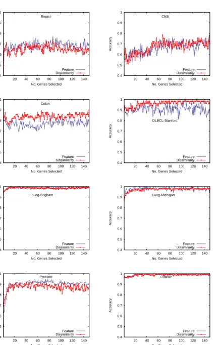
Figure 3: Classification accuracy with the SVM when varying the number of genes selected by ReliefF.

(16)

0.4 0.5 0.6 0.7 0.8 0.9 1 20 40 60 80 100 120 140 Accuracy

Figure 4: Classification accuracy with the MLP when varying the number of genes selected by ReliefF.

(17)

the Lung-Michigan database appears to be the exception that confirms the rule, since the accuracy with the dissimilarity representation suffers a very important degradation in the range between 15 and 120 selected genes when compared to the performance using the feature space.

In general, the performance of MLP models plotted in Fig. 4 seems to be little affected by the representation space used. While the Breast, Colon, DLBCL-Stanford and Prostate databases present some small differences be-tween the accuracies on the feature space and those on the dissimilarity space, the rest of problems show very similar results irrespective of the representa-tion space used to build the neural networks.

Table 3: Accuracy averaged across the 150 top-ranked genes (±standard deviation) and Friedman’s average ranks for each model.

FLD-F FLD-D SVM-F SVM-D MLP-F MLP-D Breast 0.6577±0.07 0.7205±0.03 0.7041±0.02 0.7329±0.03 0.6846±0.04 0.6518±0.04 CNS 0.5949±0.04 0.7166±0.04 0.6732±0.06 0.6755±0.05 0.6625±0.05 0.6707±0.06 Colon 0.6846±0.08 0.8260±0.02 0.7415±0.04 0.8085±0.02 0.7704±0.03 0.8374±0.03 DLBCL 0.7752±0.07 0.9413±0.03 0.9406±0.03 0.9434±0.03 0.9089±0.03 0.9624±0.03 Lung-B 0.9658±0.01 0.9863±0.01 0.9825±0.01 0.9750±0.01 0.9860±0.01 0.9856±0.01 Lung-M 0.9419±0.03 0.9744±0.02 0.9624±0.02 0.7041±0.20 0.9780±0.02 0.9723±0.02 Prostate 0.7066±0.06 0.9023±0.04 0.8932±0.06 0.8948±0.04 0.9017±0.05 0.8732±0.03 Ovarian 0.9966±0.01 0.9913±0.01 0.9941±0.01 0.9889±0.01 0.9932±0.01 0.9879±0.01 Average 0.7904 0.8823 0.8615 0.8404 0.8607 0.8677 Rank 5.125 2.000 3.625 3.375 3.250 3.625

The findings discussed so far are supported by the results in Table 3, which reports the accuracy averaged across the 150 top-ranked genes for each database, the average values across all the databases and the Friedman’s average ranks for each approach (the one with the lowest average rank has to

(18)

be viewed as the best solution). The values for the best performing method in each database are underlined. Based on the Friedman’s average ranks, the results reveal that the FLD classifier built on the dissimilarity space can be considered as the model with the best overall performance, followed by the SVM-D approach. What is more interesting, however, is that the feature-based classifiers have been worse in 6 out of the 8 databases (only FLD-F applied to the Ovarian data set and MLP-F on Lung-Michigan have been slightly superior to any other method), demonstrating the benefits of using the dissimilarity-based approaches to the classification of microarray data.

With the aim of checking whether or not the accuracy results are signifi-cantly different, the Iman-Davenport’s statistic has been computed [7]. This is distributed according to an F-distribution with K−1 and (K−1)(N−1)

degrees of freedom, where K denotes the number of models and N is the

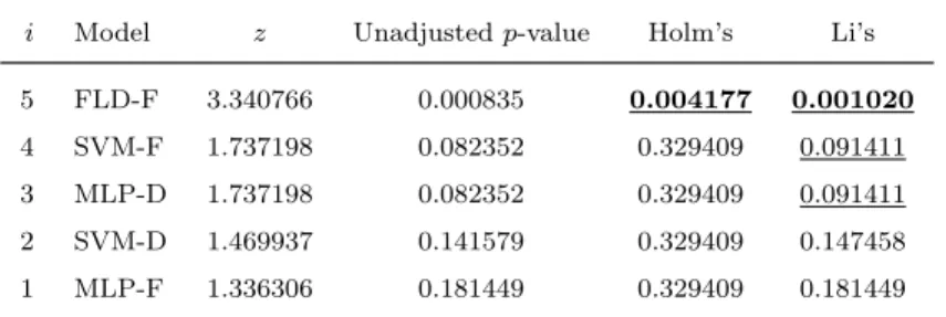
total number of data sets. The p-value computed byF(5,35) was 0.0314056, which is less than a significance level of α = 0.05. Therefore, the null-hypothesis that all the approaches perform equally well can be rejected. As the Iman-Davenports statistic only allows to figure out differences among all methods, we have also carried on with two post hoc tests (Holm’s and Li’s) using the best classifier (FLD-D) as the control algorithm [7]. Instead of the unadjusted p-values, both post hoc tests have been used with the adjusted p-values because these reflect the probability error of a certain comparison, but they do not disregard the familiy-wise error rate (the probability of mak-ing one or more false discoveries among all the hypotheses when performmak-ing multiple pairwise tests) [8, 12].

(19)

Table 4: Results obtained with Holm’s and Li’s tests (the classifiers have been sorted in ascending order of the unadjustedp-values).

i Model z Unadjustedp-value Holm’s Li’s

5 FLD-F 3.340766 0.000835 0.004177 0.001020

4 SVM-F 1.737198 0.082352 0.329409 0.091411

3 MLP-D 1.737198 0.082352 0.329409 0.091411

2 SVM-D 1.469937 0.141579 0.329409 0.147458

1 MLP-F 1.336306 0.181449 0.329409 0.181449

Li’s procedures. The methods which have been significantly worse than the control algorithm at a significance level of α = 0.05 are highlighted in bold, and those that reject the null-hypothesis of equivalence with the control algorithm for α = 0.1 are underlined. The Holm’s test detected significant pairwise differences, revealing that the FLD-D model performs significantly better than the feature-based FLD and it is statistically equivalent to the rest of methods. On the other hand, the Li’s post hoc test showed that the FLD-D scheme is significantly better than FLD-F at a significance level of α = 0.05, and significantly superior to SVM-F and MLP-D at a significance level of α = 0.1.

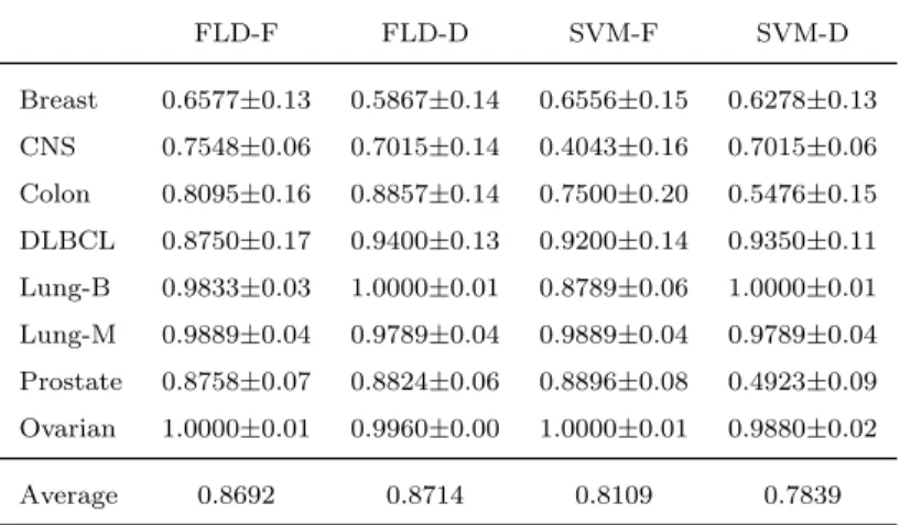
Although the aim of this work is not to choose the best performing subset of genes, Table 5 summarizes the accuracy results achieved by each classifica-tion approach when using all the genes (that is, without feature selecclassifica-tion) in order to provide a baseline for comparison with the results given in Table 3. Nonetheless, because of a lack of memory capacity in our machine, it has not been possible to report the results of the MLP models for this experiment; therefore, we have restricted the analysis to the cases of FLD and SVM. An interesting observation is that the feature-based classifiers have performed

(20)

better by using the whole set of genes than with a subset of genes, whereas the dissimilarity-based models have achieved better results after selecting the 150 top-ranked genes. This behavior may be of great relevance to real-life applications of biomedicine because the use of a smaller number of genes allows to reduce the computational burden of the classifiers and to increase theknowledgeof the relationships among genes and classes, which are in fact two important objectives of feature selection.

Table 5: Average accuracy using the original sets of genes (±standard deviation) for the FLD and SVM models. FLD-F FLD-D SVM-F SVM-D Breast 0.6577±0.13 0.5867±0.14 0.6556±0.15 0.6278±0.13 CNS 0.7548±0.06 0.7015±0.14 0.4043±0.16 0.7015±0.06 Colon 0.8095±0.16 0.8857±0.14 0.7500±0.20 0.5476±0.15 DLBCL 0.8750±0.17 0.9400±0.13 0.9200±0.14 0.9350±0.11 Lung-B 0.9833±0.03 1.0000±0.01 0.8789±0.06 1.0000±0.01 Lung-M 0.9889±0.04 0.9789±0.04 0.9889±0.04 0.9789±0.04 Prostate 0.8758±0.07 0.8824±0.06 0.8896±0.08 0.4923±0.09 Ovarian 1.0000±0.01 0.9960±0.00 1.0000±0.01 0.9880±0.02 Average 0.8692 0.8714 0.8109 0.7839

4.1. Classification results on each class

In order to visualize the accuracies on each individual class, we have also plotted the true-positive rate (x-axis) versus the true-negative rate (y-axis) in Fig. 5 for the Fisher’s linear discriminant, Fig. 6 for the SVM and Fig. 7 for the MLP neural network, using both the feature-based (blue circles) and the dissimilarity-based (red stars) representations. For each model, we have depicted 150 points, each one corresponding to a subset with the top-ranked

(21)

genes (from 1 to 150). In this manner, the best approach can be deemed as the one that accumulates a higher number of points closest to the top-right corner of the graph, which corresponds to the optimal classification (TPr = 1, TNr = 1).

Even though it may seem that there is not a pattern common to all the plots, the dissimilarity-based representation has a higher quantity of points close to the top-right corner than the feature-based representation, espe-cially in the case of the FLD classifier. This effect is particularly evident on the Colon, DLBCL-Stanford and Prostate databases. On the contrary, the Breast cancer database presents a rather confusing picture because the dissimilarity-based representation generally performs better than the feature-based FLD model, but a few number of points belonging to the feature-feature-based approach are closer to the top-right corner.

In Fig. 6, one can observe a certain overlapping between both representa-tions in most databases, which makes difficult to determine whether or not one method has been superior to the other. While the dissimilarity-based representation seems to yield better results than the feature-based repre-sentation on the Colon database, it performs clearly worse in the case of the Lung-Michigan database. In fact, these results agree with the behavior previously illustrated in Fig. 3.

Finally, the plots in Fig. 7 reveal that the behavior of the MLP neural network is more similar to that of the Fisher’s linear discriminant model than to the one of the SVM. Although the points of the dissimilarity-based and the feature-based representations are overlapped with each other for five databases, the former seems to have a larger number of points close to the

(22)

0.2 0.3 0.4 0.5 0.6 0.7 0.8 0.9 1 0.2 0.3 0.4 0.5 0.6 0.7 0.8 0.9 1 TNr TPr Breast Feature Dissimilarity 0.2 0.3 0.4 0.5 0.6 0.7 0.8 0.9 1 0.2 0.3 0.4 0.5 0.6 0.7 0.8 0.9 1 TNr TPr CNS Feature Dissimilarity 0.2 0.3 0.4 0.5 0.6 0.7 0.8 0.9 1 0.2 0.3 0.4 0.5 0.6 0.7 0.8 0.9 1 TNr TPr Colon Feature Dissimilarity 0.2 0.3 0.4 0.5 0.6 0.7 0.8 0.9 1 0.2 0.3 0.4 0.5 0.6 0.7 0.8 0.9 1 TNr TPr DLBCL-Stanford Feature Dissimilarity 0.2 0.3 0.4 0.5 0.6 0.7 0.8 0.9 1 0.2 0.3 0.4 0.5 0.6 0.7 0.8 0.9 1 TNr TPr Lung-Brigham Feature Dissimilarity 0.2 0.3 0.4 0.5 0.6 0.7 0.8 0.9 1 0.2 0.3 0.4 0.5 0.6 0.7 0.8 0.9 1 TNr TPr Lung-Michigan Feature Dissimilarity 0.2 0.3 0.4 0.5 0.6 0.7 0.8 0.9 1 0.2 0.3 0.4 0.5 0.6 0.7 0.8 0.9 1 TNr TPr Prostate Feature Dissimilarity 0.2 0.3 0.4 0.5 0.6 0.7 0.8 0.9 1 0.2 0.3 0.4 0.5 0.6 0.7 0.8 0.9 1 TNr TPr Ovarian Feature Dissimilarity

Figure 5: True-positive rate versus true-negative rate using the FLD model with the 150 top-ranked genes.

(23)

Figure 6: True-positive rate versus true-negative rate using the SVM classifier with the 150 top-ranked genes.

(24)

Figure 7: True-positive rate versus true-negative rate using the MLP neural network with the 150 top-ranked genes.

(25)

top-right corner for the remaining problems. This is especially apparent on the Colon database, and even on the DLBCL-Stanford data.

5. Conclusion

In this work, we have proposed a methodology based on the dissimilarity representation paradigm for classification of microarray gene expression data. The procedure consists of two stages: first, as a preprocessing step, the ReliefF algorithm produces a ranking of genes according to their relevance and a subset of the top-ranked genes is then selected; second, the training examples defined on the lower-dimensional feature space are mapped into a dissimilarity space, on which the corresponding classifier is finally built.

The experiments have been carried out over eight benchmark databases available in the Internet to fulfill the objectives of this study, which have pri-marily been to investigate and evaluate the classification performance of the dissimilarity-based representation as compared to the conventional feature-based models in the context of microarray data. To this end, we have used the FLD, SVM and MLP classifiers and estimated the overall classification accuracy, the true-positive rate and the true-negative rate by means of a 10-fold cross-validation scheme. In addition, we have already calculated the Friedman’s ranks of classification accuracy averaged across the 150 subsets of genes in order to ascertain whether or not the classifiers built on a dissim-ilarity space outperform those constructed on a feature space.

The reported results show that the classification models based on a dis-similarity representation have achieved higher prediction accuracy on most databases and almost independently of the number of genes. Among the

(26)

three classifiers here applied, it has to be noted that the Fisher’s linear dis-criminant appears to be the best performing algorithm and therefore it can be concluded as a suitable solution for the classification of microarray gene expression data. It is also important to remark that the dissimilarity-based approaches appear to be more robust and less sensitive to the number of genes selected than the feature-based classifiers. Hence, we believe that our experiments have demonstrated the potential benefits of using this alterna-tive representation paradigm in the realm of biomedical applications, asitis the case of the classification of cancerous and normal tissue samples or the discrimination of different (sub)types of tumors.

Although this preliminary study has concentrated on three linear clas-sifiers, we plan on testing the proposed dissimilarity-based approach using other prediction models that have already been applied to several biomedical applications. In particular, we would like to extend the present study to ensembles of classifiers because these have proven to be very effective and obtain reliable results in a number of real-life problems, including the anal-ysis and classification of microarray data. While this work has focused on the use of the Euclidean metric as a dissimilarity function, there are other distance measures that could also be explored and even pseudo-Euclidean spaces determined by an embedding procedure could be studied as well. Fi-nally, another avenue for further research refers to the analysis of the effect of imbalanced class distributions, missing values in genes, data sparsity and small disjuncts on the performance of dissimilarity-based approaches, which constitute some additional data complexities fairly common to this kind of biomedical applications.

(27)

Acknowledgment

This work has partially been supported by the Mexican Science and Technology Council (CONACYT-Mexico) through a Postdoctoral Fellow-ship [223351], the Spanish Ministry of Economy [TIN2013-46522-P] and the Generalitat Valenciana [PROMETEOII/2014/062].

References

[1] A. Ben-Hur, J. Weston, A user’s guide to support vector machines, in: O. Carugo, F. Eisenhaber (eds.), Data Mining Techniques for the Life Sciences, vol. 609 of Methods in Molecular Biology, Humana Press, New York, USA, 2010, pp. 223–239.

[2] A. Berns, Cancer: Gene expression in diagnosis, Nature 403 (2000) 491–492.

[3] V. Bonato, V. Baladandayuthapani, B. M. Broom, E. P. Sulman, K. D. Aldape, K.-A. Do, Bayesian ensemble methods for survival prediction in gene expression data, Bioinformatics 27 (3) (2011) 359–367.

[4] U. M. Braga-Neto, E. R. Dougherty, Is cross-validation valid for small-sample microarray classication?, Bioinformatics 20 (3) (2004) 374–380.

[5] B. Chandra, M. Gupta, An efficient statistical feature selection approach for classification of gene expres-sion data, J. Biomed. Inform. 44 (4) (2011) 529–535.

[6] P. C. Conilione, D. H. Wang, A comparative study on feature selection for E.coli promoter recognition, Int. J. Inf. Tech. 11 (8) (2005) 54–66.

[7] J. Demˇsar, Statistical comparisons of classifiers over multiple data sets, J. Mach. Learn. Res. 7 (1) (2006) 1–30.

[8] J. Derrac, S. Garc´ıa, D. Molina, F. Herrera, A practical tutorial on the use of nonparametric statisti-cal tests as a methodology for comparing evolutionary and swarm intelligence algorithms, Swarm Evol. Comput. 1 (1) (2011) 3–18.

[9] E. R. Dougherty, Small sample issues for microarray-based classification, Compar. Func. Genom. 2 (1) (2001) 28–34.

[10] S. Dudoit, J. Fridlyand, Classication in microarray experiments, in: T. P. Speed (ed.), Statistical Analysis of Gene Expression Microarray Data, Chapman & Hall/CRC Press, London, UK, 2003, pp. 93–158.

(28)

[11] T. S. Furey, N. Duffy, N. Cristianini, D. Bednarski, M. Schummer, D. Haussler, Support vector machine classification and validation of cancer tissue samples using microarray expression data, Bioinformatics 16 (10) (2000) 906–914.

[12] S. Garc´ıa, A. Fern´andez, J. Luengo, F. Herrera, Advanced nonparametric tests for multiple comparisons in the design of experiments in computational intelligence and data mining: Experimental analysis of power, Inf. Sci. 180 (10) (2010) 2044–2064.

[13] I. Guyon, A. Elisseeff, An introduction to variable and feature selection, J. Mach. Learn. Res. 3 (2003) 1157–1182.

[14] A. E. Hassanien, E. T. Al-Shammari, N. I. Ghali, Computational intelligence techniques in bioinformatics, Comput. Biol. Chem. 47 (0) (2013) 37–47.

[15] R. Hewett, P. Kijsanayothin, Tumor classification ranking from microarray data, BMC Genomics 9 (2) (2008) S21.

[16] J. Hua, Z. Xiong, J. Lowey, E. Suh, E. R. Dougherty, Optimal number of features as a function of sample size for various classification rules, Bioinformatics 21 (8) (2005) 1509–1515.

[17] I. Inza, P. Larra˜naga, R. Blanco, A. J. Cerrolaza, Filter versus wrapper gene selection approaches in DNA microarray domains, Artif. Intell. Med. 31 (2) (2004) 91–103.

[18] I. Kononenko, Estimating attributes: Analysis and extensions of RELIEF, in: Proceedings of the 7th European Conference on Machine Learning, Springer-Verlag, Catania, Italy, 1994, pp. 171–182.

[19] P. Larrañaga, B. Calvo, R. Santana, C. Bielza, J. Galdiano, I. Inza, J. A. Lozano, R. Armañanzas, G. Santafé, A. Pérez, V. Robles, Machine learning in bioinformatics, Brief. Bioinform. 7 (1) (2011) 86– 112.

[20] D.-C. Li, Y.-H. Fang, Y.-Y. Lai, S. C. Hu, Utilization of virtual samples to facilitate cancer identification for DNA microarray data in the early stages of an investigation, Inf. Sci. 179 (16) (2009) 2740–2753.

[21] T. Li, C. Zhang, M. Ogihara, A comparative study of feature selection and multiclass classification meth-ods for tissue classification based on gene expression, Bioinformatics 20 (15) (2004) 2429–2437.

[22] Y. Lu, J. Han, Cancer classification using gene expression data, Inform. Syst. 28 (4) (2003) 243–268.

[23] S. Ma, J. Huang, Regularized ROC method for disease classification and biomarker selection with mi-croarray data, Bioinformatics 21 (2) (2005) 4356–4362.

[24] P. Mahata, K. Mahata, Selecting differentially expressed genes using minimum probability of classification error, J. Biomed. Inform. 40 (6) (2007) 775–786.

(29)

[25] R. M. Parry, W. Jones, T. H. Stokes, J. H. Phan, R. A. Moffitt, H. Fang, L. Shi, A. Oberthuer, M. Fischer, W. Tong, M. D. Wang, k-Nearest neighbor models for microarray gene expression analysis and clinical outcome prediction, Pharmacogenomics J. 10 (4) (2010) 292–309.

[26] E. P¸ekalska, R. P. W. Duin, Dissimilarity representations allow for building good classifiers, Pattern Recogn. Lett. 23 (8) (2002) 943–956.

[27] E. P¸ekalska, R. P. W. Duin, The Dissimilarity Representation for Pattern Recognition: Foundations and Applications, World Scientific, Singapore, 2005.

[28] E. Pekalska, R. P. W. Duin, P. Pacl´ık, Prototype selection for dissimilarity-based classifiers, Pattern Recogn. 39 (2) (2006) 189–208.

[29] E. P¸ekalska, P. Paclik, R. P. W. Duin, A generalized kernel approach to dissimilarity-based classification, J. Mach. Learn. Res. 2 (2002) 175–211.

[30] E. Raspe, C. Decraene, G. Berx, Gene expression profiling to dissect the complexity of cancer biology: Pitfalls and promise, Semin. Cancer Biol. 22 (3) (2012) 250–260.

[31] S. J. Raudys, A. K. Jain, Small sample size effects in statistical pattern recognition: Recommendations for practitioners, IEEE T. Pattern Anal. Mach. Intell. 13 (3) (1991) 252–264.

[32] M. Ringner, C. Peterson, Microarray-based cancer diagnosis with artificial neural networks, Biotechniques 34 (S3) (2003) 30–35.

[33] M. Robnik-ˇSikonja, I. Kononenko, Theoretical and empirical analysis of ReliefF and RReliefF, Mach. Learn. 53 (1-2) (2003) 23–69.

[34] Y. Saeys, I. Inza, P. Larra˜naga, A review of feature selection techniques in bioinformatics, Bioinformatics 23 (19) (2007) 2507–2517.

[35] A. V. Sousa, A. M. Mendon¸ca, A. Campilho, Dissimilarity-based classification of chromatographic profiles, Pattern Anal. Appl. 11 (3–4) (2008) 409–423.

[36] X. Sun, Y. Liu, D. Wei, M. Xu, H. Chen, J. Han, Selection of interdependent genes via dynamic relevance analysis for cancer diagnosis, J. Biomed. Inform. 46 (2) (2013) 252–258.

[37] L.-J. Tang, W. Du, H.-Y. Fu, J.-H. Jiang, H.-L. Wu, G.-L. Shen, R.-Q. Yu, New variable selection method using interval segmentation purity with application to blockwise kernel transform support vector machine classification of high-dimensional microarray data, J. Chem. Inf. Model. 49 (8) (2009) 2002–2009.

[38] A. Ula¸s, R. P. W. Duin, U. Castellani, M. Loog, P. Mirtuono, M. Bicego, V. Murino, M. Bellani, S. Cerruti, M. Tansella, P. Brambilla, Dissimilarity-based detection of schizophrenia, Int. J. Imag. Syst. Tech. 21 (2) (2011) 179–192.

(30)

[39] S.-L. Wang, Y.-H. Zhu, W. Jia, D.-S. Huang, Robust classification method of tumor subtype by using correlation filters, IEEE/ACM T. Comput. Bi. 9 (2) (2012) 580–591.

[40] B. Weigelt, F. L. Baehner, J. S. Reis-Filho, The contribution of gene expression profiling to breast cancer classification, prognostication and prediction: a retrospective of the last decade, J. Pathol. 220 (2) (2010) 263–280.

[41] Y. Yoon, J. Lee, S. Park, S. Bien, H. C. Chung, S. Y. Rha, Direct integration of microarrays for selecting informative genes and phenotype classification, Inf. Sci. 178 (1) (2008) 88–105.

[42] J.-G. Zhang, H.-W. Deng, Gene selection for classification of microarray data based on the Bayes error, BMC Bioinformatics 8 (2007) 370.