A Restricted Bi-factor Model of Subdomain Relative Strengths and Weaknesses
A DISSERTATION
SUBMITTED TO THE FACULTY OF THE GRADUATE SCHOOL OF THE UNIVERSITY OF MINNESOTA
BY
Yu-Feng Chang
IN PARTIAL FULFILLMENT OF THE REQUIREMENTS FOR THE DEGREE OF
DOCTOR OF PHILOSOPHY Mark L. Davison
i
Acknowledgements
In this long journey of obtaining my PhD, there are a lot of people I want to express my appreciation to. Especially, I would like to thank my advisor, Mark Davison, for his mentoring and support. Without him, I would not have been able to finish my degree. I have learned many things from him, and I am still learning more and more with each discussion we have. I thank you more than what words can describe here.
Also, I would like to thank my committee members, Ernest Davenport, Chun Wang, Andy Zieffler, and Michael Rodriguez for their thoughtful feedback during every stage of building my dissertation. I thank you for your knowledge and insight.
Likewise, I would like to thank my friends and cohort members in the QME program. I have learned more from you than any books. I thank you for what you have done to enrich my life.
Finally, I would like to the Chang family and Berry family, because of your support and positive thoughts, I was able to complete my dissertation.
ii Dedication
To my family: my father, who is supportive; my husband, who is patient; my daughter, who is sweet.
iii Abstract
There are increasing demands to report subscores in educational and
psychological assessments. Subscores provide unique information about examinees (Sinharay, Puhan & Haberman, 2011). However, there has been much debate about reporting subscores because subscores require meeting certain standards and
psychometric qualities as a prerequisite to reporting them. Because there is an increasing need for improving the methods of estimating subscores, multidimensional item response theory (MIRT) is one of the methods to estimate subscores.
One MIRT model is the item bi-factor model, which includes a general dimension on which all items load and specific dimensions corresponding to the subdomains from which the items come (Holzinger & Swineford’s, 1937; Gibbons & Hedeker, 1992). However, there is a challenge to interpreting the specific dimension scores in the item bi-factor model while the general dimension score is readily interpreted. The specific dimension scores are residuals from the general factor and residuals can be difficult to interpret.
To solve this issue, a restricted bi-factor model was proposed in this paper. This paper contains a real data study and a simulation study to evaluate this model. The results of two studies, interpretation of the model, and practical application of the model were discussed.
iv
Table of Contents
Acknowledgements i
Dedication ii
Abstract iii
List of Tables viii
List of Figures x
Chapter I: Introduction 1
Statement of the Problem . . . 1
Significance of the Study . . . . . . 3
Chapter II: Literature Review 5
Introduction . . . 5
Unidimensional Item Response Theory . . . 6
Multidimensional Item Response Theory . . . 8
Multidimensional Extension of the Three-Parameter Logistic Model . . . 9
Multidimensional Extension of the Two-Parameter Logistic Model . . . 10
Multidimensional Extension of the Rasch Model . . . 10
Latent Variable Models . . . 11
Connection between the MIRT Models and Full-information Item Factor Analysis. . . 14
Full-Information Item Factor Analysis . . . 14
v
Item Parameter Estimation . . . 17
Marginal Maximum Likelihood . . . 17
Expectation/Maximization (EM) algorithm . . . 19
Person Parameter Estimation . . . 20
Maximum Likelihood Estimation . . . 20
Bayesian Methods . . . 23
The Bi-factor Model . . . 25
Full-Information Item Bi-factor Analysis . . . 26
The bi-factor model in the IRT framework . . . 28
Studies of Application . . . 29
Studies of Estimation Algorithm . . . 34
Studies of Simulation . . . .. . . 35
Summary . . . 37
Chapter III: Method 40
Method . . . 41
A Restricted bi-factor model . . . .43
Estimating the General and Specific Dimensions Scores. . . 44
Estimating the Variances and Covariances among the Dimensions . . . . .44
Estimating the Conditional Error Variances and Covariances among Dimensions. . . 45
Interpretation of the general and specific dimension scores . . . .45
vi Participants . . . 47 Measures. . . 47 Simulation Study. . . 48 Simulation Conditions . . . 48 Simulation Procedures . . . 50 Data Generation . . . 50 Simulation Phase . . . .52 Evaluation Criteria . . . 53
Chapter IV: Results 57
Results of Real Data Study. . . 57
Results of Simulation Study. . . 61
Correlation between two Numbers of Quadrature Points. . . 62
Correlation between the MAP and the EAP. . . 62
Comparison between Variances of the MAP and the EAP Scores. . . 64
Variance of the True Restricted Bi-factor Scores . . . .66
Bias and Absolute Bias. . . 67
The RMSE and the SE. . . .70
Average Conditional Error Variance. . . .75
Reliability. . . .77
Sensitivity and Specificity of the Score, zpj. . . 79
Chapter V: Conclusion 82
vii
Conclusion of Simulation Study . . . .85
Limitations. . . .87 Future Work . . . 88 Application . . . 89 Final Thoughts . . . ..90 References 91 Appendix A 100 Proof 1 . . . . . . 100 Proof 2 . . . . . . 102 Appendix B 104
viii List of Tables
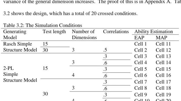
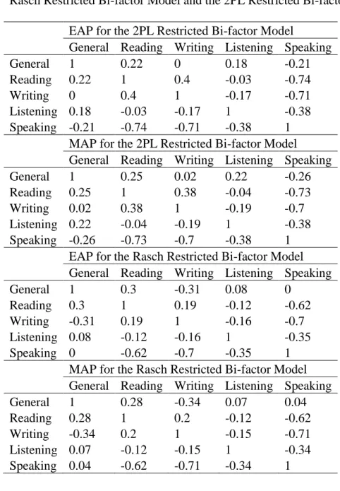
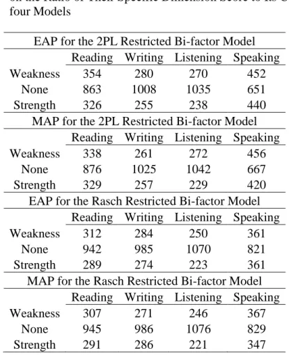
Table 3.1: Number of Items for Each Domain . . . 48 Table 3.2: The Simulation Conditions . . . 50 Table 3.3: Cut-off Points for a True Strength or Weakness and a Significant Strength or Weakness. . . .56 Table 4.1: Within Model Correlation Matrices: MAP and EAP Person Scores for the Rasch Restricted Bi-factor Model and the 2PL Restricted Bi-factor Model. . . .58 Table 4.2: Cross Model Correlation Matrices: MAP and EAP Person Scores for the Rasch Restricted Bi-factor Model and the 2PL Restricted Bi-factor Model. . . 59 Table 4.3: The Reliability of MAP and EAP Person Scores for the Rasch Restricted Bi-factor Model and the 2PL Restricted Bi-Bi-factor Model. . . 60 Table 4.4: Number of People Identified with a Significant Strength or Weakness Based on the Ratio of Their Specific Dimension Score to Its Conditional Standard Error for the four Models. . . 61 Table 4.5: Correlation for Each Dimension and for the SE of Each Dimension between Two Sets of Quadrature Points. . . 62 Table 4.6: Correlations for Each Dimension between the EAP and MAP Estimation
methods. . . 63 Table 4.7: Correlations for the SE of Each Dimension for the EAP and MAP Estimation Methods. . . 63 Table 4.8: Variance of the MAP and Variance of the EAP. . . .65 Table 4.9: Variance of the True Restricted Bi-factor Score. . . 66
ix
Table B.1: Bias of Each Dimension Score for Cell 1 to Cell 20. . . .105
Table B.2: Absolute Bias of Each Dimension Score for Cell 1 to Cell 20. . . 110
Table B.3: RMSE of Each Dimension Score for Cell 1 to Cell 20. . . 115
Table B.4: SE of Each Dimension Score for Cell 1 to Cell 20. . . 120
Table B.5: Average MSE of Each Dimension Score for Cell 1 to Cell 20. . . 125
Table B.6: Reliability and MSE of Each Dimension Score for Cell 1 to Cell 20. . . 130
Table B.7: Sensitivity for the Strength and Weakness and Specificity of Each Dimension Score for Cell 1 to Cell 20. . . .132
x List of Figures
Figure 2.1: Between-item Multidimensionality Models and Within-item
Multidimensionality Models. . . .11
Figure 2.2: Four Latent Variable Models. . . 13
Figure 2.3: Higher-order Factor Models and Hierarchical Factor Models. . . 14
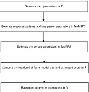
Figure 3.1: Simulation Phase of the Study. . . .53
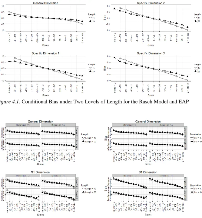
Figure 4.1: Conditional Bias under Two Levels of Length for the Rasch Model and EAP . . . 68
Figure 4.2: Conditional Bias under Various Conditions of Length and Correlation for the 2PL Model and EAP. . . 68
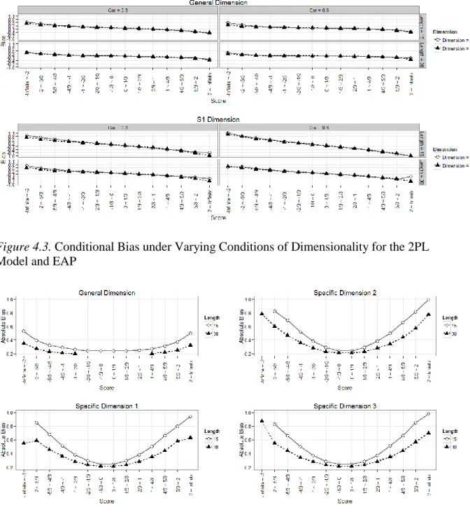
Figure 4.3: Conditional Bias under Varying Conditions of Dimensionality for the 2PL Model and EAP. . . 69
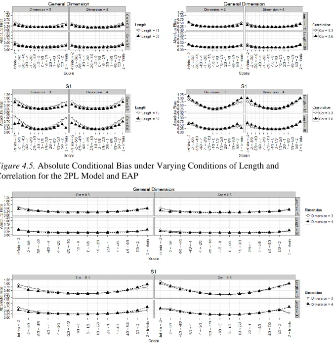
Figure 4.4: Absolute Conditional Bias under two Levels of Length for the Rasch Model and EAP. . . .69
Figure 4.5: Absolute Conditional Bias under Varying Conditions of Length and Correlation for the 2PL Model and EAP. . . .70
Figure 4.6: Absolute Conditional Bias under Varying Conditions of Dimensionality for the 2PL Model and EAP. . . 70
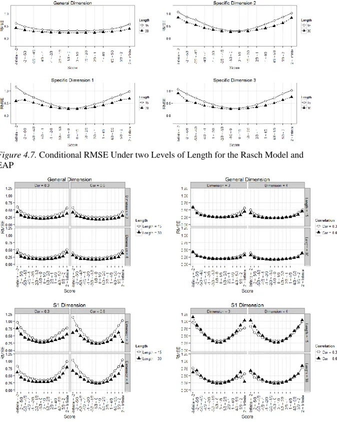
Figure 4.7: Conditional RMSE Under two Levels of Length for the Rasch Model and EAP. . . 72
Figure 4.8: Conditional RMSE under Varying Conditions of Length and Correlation for the 2PL Model and EAP. . . 72
xi
Figure 4.9: Conditional RMSE under Varying Conditions of Dimensionality for 2PL Model and EAP. . . 73 Figure 4.10: Conditional SE Under two Levels of Length for the Rasch Model and EAP . . . 73 Figure 4.11: Conditional SE under Varying Conditions of Length and Correlation for the 2PL Model and EAP. . . 74 Figure 4.12: Conditional SE under Varying Conditions of Dimensionality for the2PL Model and EAP. . . 74 Figure 4.13: Average Conditional MSE Under Two Levels of Length for the Rasch Model and EAP. . . 75 Figure 4.14: Average Conditional MSE under Varying Conditions of Length and
Correlation for the Condition of the 2PL Model and EAP. . . 76 Figure 4.15: Average Conditional MSE for the Condition of Dimensionality and the Condition of the 2PL Model and EAP. . . .76 Figure 4.16: Reliability Under two Levels of Length for the Rasch Model and EAP. . . .78 Figure 4.17: Reliability under Varying Conditions for the 2PL Model and EAP. . . .78 Figure 4.18: Sensitivity and Specificity for True Strengths and Weaknesses Under two Levels of Length for the Rasch Model and EAP. . . .79 Figure 4.19: Sensitivity to Strengths under Varying Conditions for the 2PL Model and EAP. . . 80 Figure 4.20: Sensitivity to Weaknesses under Varying Conditions for the 2PL Model and EAP. . . 81
xii
1
Chapter I: Introduction
Statement of the Problem
There are increasing demands to report subscores in educational and psychological assessments. According to the National Research Council report
“Knowing What Students Know” (2001), the target of assessment is to provide particular information about an examinee’s knowledge, skill, and abilities. Subscores provide unique information about examinees (Sinharay, Puhan & Haberman, 2011). Various audiences see the usefulness of subscores. For test takers, subscores are desirable because they can provide strengths and weaknesses about examinees’ abilities and skills to help with future remedial studies. For educators, subscores can suggest remedies for examinees lacking certain abilities. For state and academic institutions, subscores could be tools to evaluate a curriculum’s effectiveness. For college and university admission officers, subscores can provide distinct information for admission purposes when candidates have similar total scores. For policy makers, subscores may be guides to change state curriculums and provide more funding in different content areas (Haladyna & Kramer, 2004; Leading & Monaghan, 2006).
However, there has been much debate about reporting subscores in the field of educational and psychological assessment because subscores require meeting certain standards and psychometric qualities as a prerequisite to reporting them. Standard 5.12 of the Standards for Educational and Psychological Testing (American Educational Research Association, American Psychological Association, & National Council on Measurement in Education, 1999) states: “Scores should not be reported for individuals
2
unless the validity, comparability, and reliability of such scores have been established.” Moreover, Standard 1.12 of the same document states: “If a test provides more than one score, the distinctiveness of the separate scores should be demonstrated.” Also, Standard 2.1 states: “For each total score, subscores, or combination of scores that is to be
interpreted, estimates of relevant reliabilities and standard errors of measurement or test information functions should be reported” (AERA, APA, NCME, 1999). Inaccurate information about subscores or reporting subcores without proper interpretation could lead to inaccurate decisions.
The reasons that subscores may lack psychometric qualities are as follows. First, there may not be enough items within each domain. Tate (2004) stated sufficient validity and reliability for subscores can minimize incorrect individual instructional decisions. Second, subscores in educational measurements often refer to domain areas. If an assessment with several domains is constructed to measure a single construct, little reason exists to expect useful subscores (Sinharay, Puhan & Haberman, 2011). In this case, correlations between domains tend to be relatively high. Correlations between domains may be a sign that the assessment is unidimensional.
Once the psychometric quality and number of dimensions of assessments are assured, several alternatives can be used to compute subscores. Multidimensional item response theory (MIRT) is one method to estimate subscores. Ability estimation using the MIRT method and augmentation methods perform best in estimating the true subscores compared to other methods (Dwyer, Boughton, Yao, Steffen, & Lewis, 2006; Fu & Qu, 2010). Yao and Boughton (2007) showed that MIRT ability estimation
3
performs better than percentage or number-correct or the objective performance index (OPI), which is a unidimensional IRT subscale scoring approach.
One of the multidimensional item response theory models is the item bi-factor model. One of the advantages for the item bi-factor model is that it accounts for a general dimension on which all items load and specific dimensions corresponding to the subdomains from which the items come (Holzinger & Swineford’s, 1937; Gibbons & Hedeker, 1992). However, there is a challenge to interpreting the specific dimension scores in the item bi-factor model while the general dimension score is readily interpreted. The specific dimension scores are residuals from the general factor and residuals can be difficult to interpret (see Chapter 2).
Standard 2.1 states: “For each total score, subscores, or combinations of scores that is to be interpreted, estimates of relevant reliabilities and standard errors of
measurement or test information functions should be reported” (AERA, APA, NCME, 1999). Reporting subscores should be interpetable or it is not worth reporting them. In other words, it is a big drawback to apply the item bi-factor model since it is difficult to interpret its subscores.
Significance of the Study
The purpose of this dissertation is to develop a restricted bi-factor model in which the general dimension represents the examinee’s overall performance in a domain, and each specific dimension represents a deviation from that overall performance. The specific dimension scores describe the examinee’s pattern of strengths and weaknesses relative to the examinee’s overall performance.
4
Moreover, the real data study in this dissertation is to demonstrate the method of the restricted bi-factor model and how to interpret the general dimension score and the specific dimension scores. The simulation study aims to answer the following research questions.
1. How are reliability, sensitivity, specificity, and recovery of person parameters, influenced by the level of correlation between dimensions?
2. How are reliability, sensitivity, specificity, and recovery of person parameters, influenced by the number of items in the test?
3. How are reliability, sensitivity, specificity, and recovery of person parameters, influenced by the number of dimensions in the test?
Chapter 2 reviews the literature, including the unidimensional item response theory (UIRT) and multidimensional item response theory (MIRT) models, the
connection between factor analysis and IRT, person parameters estimation, the bi-factor model and application, and the use of subscores. This study presents a new approach to modeling subscores. Chapter 3 describes the method of the restricted bi-factor model that is demonstrated with real and simulated data. The conditions of the simulation study, details of the real data study, and evaluation criteria are described in Chapter 3. Chapter 4 presents the results of the real data study and simulation study. Chapter 5 concludes with a discussion of the results and implications for the field of educational and psychological measurement.
5
Chapter II: Literature Review
Introduction
There are many advantages to implementing the bi-factor multidimensional IRT model on multidimensional data. However, a majority of the literature on
multidimensional IRT has focused on estimation and interpretation of the item
parameters whereas interpretation of person parameters has rarely been emphasized. For example, Simms, Grös, Watson, and O’Hara (2008) applied the bi-factor model on the inventory of depression and anxiety symptoms. This study compared the bi-factor model and the one-factor model. This study only covered magnitudes of the general and
specific factor loadings and item difficulty parameters. Nevertheless, this study only discussed the estimation method of person parameter and person scores of the general factor. According to Standard 2.1 of the Standards for Educational and Psychological Testing each total score, subscores, or combination of scores should be interpreted. Moreover, interpretation of the person parameters can be more meaningful, especially in diagnosing examinees’ strengths and weaknesses and providing useful feedback for examinees on the specific domains of the assessments. This study demonstrates a restricted bi-factor IRT model, which can be a good approach to providing meaningful person parameters and feedback on individual differences.
This chapter reviews previous research to provide background for the restricted bi-factor model. The first section below reviews unidimensional item response theory (UIRT) and multidimensional item response theory (MIRT). The second section below illustrates the connection between factor analysis and IRT. The third section below
6
conceptualizes item parameters estimation and person parameter estimation. Lastly, the fourth section reviews the bi-factor model, including the full-information item bi-factor analysis, the factor model in the IRT framework, and some studies applying the bi-factor model.
Unidimensional Item Response Theory (UIRT)
The critical restriction for traditional IRT (UIRT) is the unidimensional assumption meaning the construct of measurement contains only a single ability. In educational assessment fields, math assessments are a very noticeable example of multidimensionality. Under the traditional IRT assumption, only overall math ability is measured on math assessments although math assessments have a strong connection to reading ability. As the math example shows, the unidimensional assumption does not always hold. In other words, there could be more than one dimension underlying personality and educational assessments.
Item response theory (IRT) uses latent traits of individuals and items as predictors of observed responses. The major advantage of IRT is that person parameters and item parameters in IRT are located on the same scale. IRT has been commonly used in educational and psychological measurement. However, traditional IRT has three strong assumptions. The three assumptions under traditional IRT are unidimensionality, local independence, and functional form. First, the unidimensionality assumption means only one ability or one trait is measured by examinees’ performance on a set of items. Nevertheless, in a real application, there will most likely be some degree of violation of the unidimensionality assumption. The degree of violation may or may not be an issue. If the violation is severe, unidimensional IRT may not be useful. Instead,
7
multidimensional IRT models should be considered. Second, the assumption of local independence is that, conditional on ability level, how a person responds to an item is independent of responses to any other items. Under unidimensionality local
independence can be explained as how the examinee responds to an item only depends on the examinee’s latent traits, not how the examinee answers any other questions. The third assumption is functional form, which is the function specified by the model relating responses to traits or abilities (De Ayala, 2009).
The assumption of unidimensionality among the three assumptions is more critical since this assumption is always violated to some degree. However, the severe violation of this assumption may produce incorrect estimation as well as incorrect interpretations. In this situation, multidimensional IRT models should be used instead. The simple logistic forms with the one-parameter logistic (1PL), two-parameter logistic (2PL), and three-parameter logistic (3PL) are stated below. The 2-parameter normal ogive model is 2 1 ( 1| , , ) exp 2 2
z ij j i i z P x a b dz (2.1) where zai(jbi), aiis the item discrimination parameter, biis the difficultyparameter, and P x( ij 1|j, , )a bi i is the probability of person j answering correctly item i. Using the logistic form, the 2-parameter model can be expressed
( 1| , , ) exp[1.7 ( )] 1 exp[1.7 ( )] i j i ij j i i i j i a b P x a b a b (2.2) where 1.7 is a scaling factor.
8 ( 1| , , ) exp[1.7 ( )] 1 exp[1.7 ( )] j i ij j i j i a b P x b a a b (2.3) In the 1PL model, items have a constant value for the discrimination parameter (a). One of the 1PL models is the Rasch model for which the discrimination parameter (a) is equal to 1.
The 3-parameter logistic model (Birnbaum, 1968) is
( 1| , , , ) (1 ) exp[1.7 ( )] 1 exp[1.7 ( )] i j i ij j i i i i i i j i a b P x a b c c c a b (2.4)
where ciis the lower asymptote parameter (the guessing parameter) for the item.
Multidimensional Item Response Theory (MIRT)
Multidimensional IRT (MIRT) means the test manifests the influence of more than one latent trait. From the model point of view, each examinee has several abilities and each item has several discrimination parameters but only one guessing parameter and one intercept. There are three assumptions in the MIRT model: a functional form
assumption, the conditional independence assumption, and a dimensionality assumption. A functional form assumption means the data follow the function specified by the model. The second assumption, the conditional independence, indicates that the conditional distributions of the item responses are all independent of each other (Lord & Novick, 1968). Third, a dimensionality assumption states that the observations on the variable are a function of a set of continuous latent person variable. Essentially, dimensionality assessment is required prior to MIRT analysis (De Ayala, 2009).
9
There are two types of multidimensional IRT models. One is the compensatory model (Rasch, 1960; Reckase, 1972) and the other is the non-compensatory model (Sympson, 1978; Whitely, 1980). The compensatory model has an assumption that high ability on one dimension can compensate for low ability on another dimension in terms of probability of correct response whereas the non-compensatory model implies that
answering the item correctly required the ability on each dimension to have non-zero probability. The compensatory model is based on a linear combination of
-coordinates which yield the same sum with different combinations of
-values. Take an item with two dimensions for example. For the non-compensatory model, a person with very high ability on one dimension and very low ability on the other dimension has very low probability of answering correctly on this item. However, for the compensatory model, the same person has some substantial probability of answering the item correctly (Ansley & Forsyth, 1985; Reckase, 2009). The compensatory model is more dominant in the application research literature, and it is connected to factor analysis. In addition, it is difficult to estimate the non-compensatory model parameters (Spray, Davey, Reckase, Ackerman & Carlson, 1990). Because this study focused on compensator MIRT models for dichotomous items, several compensatory MIRT models for dichotomous items are described here.Multidimensional Extension of the Three-Parameter Logistic Model (M3PL). The most used and updated compensatory multidimensional extension of the
three-parameter logistic model (M3PL) modified by Reckase (1985) is
( 1| , , , ) (1 ) exp[1.7( )] 1 exp[1.7( )] i j i ij j i i i i i i j i d P x c d c c d a θ θ a a θ (2.5)
10 where 1 m i j ik jk k a
a θ , aiis a 1mvector of item discrimination parameters which can also be called slope parameters, j is a 1mvector of person parameters, m is the number of dimensions, ciis the lower asymptote parameter (the guessing parameter), anddiis an intercept parameter. An overall discrimination index is defined as the multidimensional discrimination index (MDISC; Reckase, 1985).
MDISC 2 1
m ik k a (2.6) MDIFF in MIRT models, which has the same interpretation as the b-parameter in UIRT is given by Equation 2.7. MDIFF 2 1
m ik k d a (2.7)Multidimensional Extension of the Two-Parameter Logistic Model (M2PL). The M2PL is obtained by setting the lower asymptote parameter (ci) to 0 in Equation 2.5.
Multidimensional Extension of the Rasch Model. The multidimensional extension of the Rasch Model is obtained by constraining the lower asymptote parameter (ci) to 0 and the discrimination parameters (aik) to 1.0 in Equation 2.5. This model becomes a UIRT version of Rasch model when m = 1 (Reckase, 2009). Moreover, Adams, Wilson, and Wang (1997) proposed the multidimensional generalization of the Rasch model, the multidimensional random coefficients multinomial logit model (MRCML). The general form of this model can be applied to dichotomous and polytomous items. The MRCML for dichotomous items is identical to theM2PL.
11
However, the discrimination parameters for the M2PL are estimates from the data, whereas the discrimination parameters for the MRCML are specified by the test
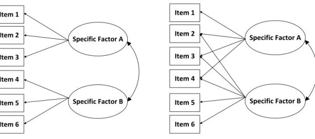
developer (Adams, Wilson & Wang, 1997; Reckase, 2009). Adams, Wilson, and Wang (1997) introduced two models in term of test structure, between-item multidimensionality models and within-item multidimensionality models. Between-item multidimensionality models, which are also called simple structure models or multi-unidimensonal models, contain several unidimensional subscales. Within-item multidimensionality models (complex structure models) contain items each of which relates to more than one dimension (Adams, Wilson & Wang, 1997; Wang, Chen, & Cheng, 2004). Figure 2.1 illustrates between-item multidimensionality models and within-item multidimensionality models.
Figure 2.1. Between-item Multidimensionality Models and Within-item Multidimensionality Models Item 2 Item 4 Item 3 Item 5 Item 6 Item 1 Specific Factor A Specific Factor B Item 2 Item 4 Item 3 Item 5 Item 6 Item 1 Specific Factor A Specific Factor B
Model A: A Between-item Model Model B: A Within-item Model Latent Variable Models. Factor analysis and MIRT have essentially identical mathematical formulas. Four major types of latent variable models for confirmatory
12
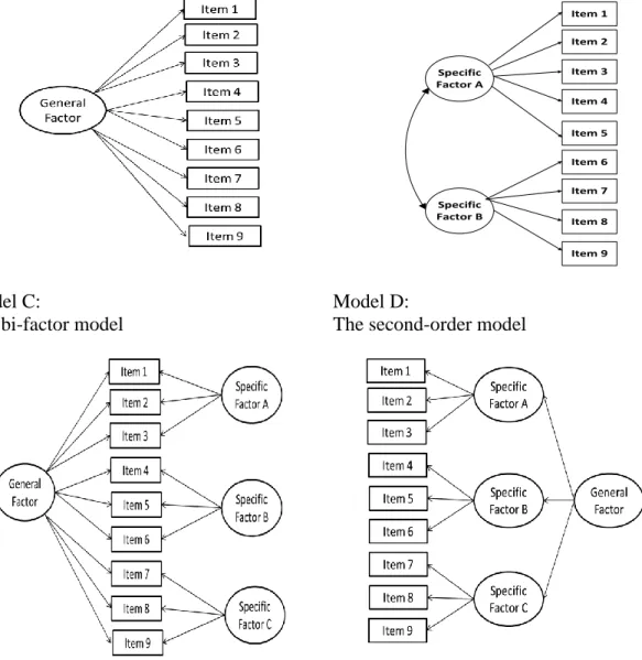
factor analysis are reviewed here (e.g., Rindskopf & Rose, 1988; Chen, West & Sousa, 2006; Reise, Morizot & Hays, 2007; Rijmen, 2010). These models are graphically represented in Figure 2.2. Model A is the multi-unidimensional model in which all the item responses can be accounted for by one common factor. Model A can also be represented as a unidimentional IRT model. Model B is the complex multidimensional model. There are two common factors in the model and the common factors are correlated with each other. The item intercorrelatons can be explained by the multiple correlated traits here. In Figure 2.2, Model C is the bi-factor model. There is one general factor and three specific factors. The general factor and the specific factors are
orthogonal in the bi-factor model. After accounting for the general factor, the specific factors explain variance over and above the general factors. The general factor in the bi-factor model explains the item intercorrelations across domains. The specific bi-factors are independent of each other in the bi-factor model because the item intercorrelaitons
already are accounted for by the general factor. Model D is the second-order model. The second-order model and the bi-factor model are both used for assessments with multiple highly related domains. They both have similar factor structures. However, the second-order model is potentially applicable when lower-second-order factors (the specific factors) are substantially correlated with each other and the higher-order factor (the general factor) accounts for the relationship among the lower-order factors and the higher-order factor is linearly dependent on the lower-order factors.
The second-order model is also called a high-order model and the hierarchical model is a special case of the bi-factor model. The relationship between the higher-order
13
factor model and the hierarchical factor model was studied by Yung, Thissen, & McLeod, (1999).
Schmid and Leiman (1957) proposed a Schmid-Leiman transformation for deriving hierarchical factor solutions from higher-order factor solutions with a simple factor clusters structure.
Figure 2.2. Four Latent Variable Models Model A:
The unidimensional model
Model B:
The non-hierarchical multidimensional model Item 2 Item 4 Item 3 Item 5 Item 6 Item 8 Item 9 Item 1 Specific Factor A Specific Factor B Item 7 Model C:
The bi-factor model
Model D:
14
The study showed that the Schmid-Leiman transformation produces a- constrained hierarchical factor solution. An unconstrained hierarchical factor model is an equivalent higher-order factor model with direct effects (loadings) on the manifest variables from the higher-order factors. Hence, the class of higher-order factor models (without direct effects of higher-order factors) is nested within the class of unconstrained hierarchical factor models. These models are graphically represented in Figure 2.3.
Figure 2.3. Higher-order Factor Models and Hierarchical Factor Models
G Item 2 Item 4 Item 3 Item 5 Item 6 Item 8 Item 7 Item 9 Item 1 F1* F2* F3* b2 b1 Item 2 Item 4 Item 3 Item 5 Item 6 Item 8 Item 7 Item 9 Item 1 F1 F2 F3 G G P2 P1 Item 2 Item 4 Item 3 Item 5 Item 6 Item 8 Item 7 Item 9 Item 1 F1* F2* F3*
Model A: Model B: Model C: A General Hierarchical Factor A Higher-order Factor Model A Higher-order Factor Model Model with Direct Effects Connection between the MIRT Models and Full-information Item Factor Analysis
The MIRT models can be re-parameterized as an item factor model. Item factor analysis does not require calculating inter-item correlation coefficients and is not strongly restricted by the number of items. Essentially, item factor analysis is the classical linear factor model adapted for binary items (Bock, & Aitkin, 1981; Bock, Gibbons, & Muraki, 1988).
Full-Information Item Factor Analysis (FIIFA). Full-information item factor analysis (FIIFA) was developed by Bock, Gibbons and Muraki (1988). Full-information
15
item factor analysis uses the frequencies of all distinct item response vectors
(Bartholomew, 1980). In contrast, the limited-information method is based on low-order joint occurrence frequencies of the item scores (Cristoffersson, 1975).
The full-information item factor analysis is adopted from Thurstone’s multiple– factor model, which assumes the M-factor model. Thurstone’s multiple–factor model is as follows:
yij i1 1j i2 2j ... im mj ij (2.8)
ij ~N(0,
i2)where yij is response of person j to item i and ijis an error term . The method posits a correct response of person j to item i when yij equals or exceeds ias a threshold and yields an incorrect response otherwise. The full-information item factor model is the probability of an item score, xij 1, which is a correct response of person j to item i with abilities j ( 1j, 2j,...,mj). (P xij 1|j) (2.9) 2 1 1 1 1 exp ( ) 2 2 i m m i ik kj i ik kj k k i i j i i i y dy
yi ~N(0,1)where iis a threshold of item i, ikis the factor loading of item i for kj, 2 i
is the error variance, and yi is the latent variable. The sample of examinees is drawn from a
16
isj MVN(0, )I , but this assumption might be relaxed to have correlated factors and a non-normal distribution. If the incorrect response isxij0, the conditional probability can be written as1 i(j) (Bock, & Aitkin, 1981; Bock, Gibbons, & Muraki, 1988).
Estimation of the Item Thresholds and Factor Loadings. Takane and De Leeuw (1987) proved the equivalence of the marginal likelihood of the two-parameter normal ogive model of multidimensional item response theory and the factor analysis of dichotomized variables. Therefore, estimation of the item thresholds and factor loadings in item factor analysis can be obtained based on the two-parameter normal ogive model of MIRT. The 2PL version of MIRT is shown in Equation 2.10.
2 ( ) 1 ( 1| , ) exp 2 2 i ij i i d t P x d dt d
i j j i i j a θ θ ,a a θ (2.10)The parameters aik and diin IRT (Equation 2.10) can be parameterized in terms of the parameters i, i and ikin the item factor analysis as Equation 2.11.
1 1 m i ik jk m k ik jk i k i a d
(2.11) The parameters aik and diin MIRT are related to the item factor parameters as follows:ik ik i a and i i i d .
There are several advantages of using the MIRT approach rather than factor analysis. First, there are less parameters being estimated in the MIRT framework. Only two parameters are estimated in the MIRT framework versus the three parameters
17
estimated in item factor analysis. Second, factor analysis is primarily a technique for data reduction while MIRT is a technique for modeling the interaction between person and test items. Reckase and Hirsch (1991) found that having less dimensions could degrade information of item and person parameters interaction, but more dimensions doesn’t cause severe problems. Consequently, MIRT might be a better tool than factor analysis because factor analysis is viewed as a data reduction tool. Also, MIRT analysis uses the same latent space across tests and samples. All analyses can be on a common coordinate system so item parameters for all items are on common metrics (Takane & De Leeuw, 1987; Reckase & Hirsch, 1991; Reckase 2009).
Item Parameter Estimation
Marginal Maximum Likelihood. Item parameters can be estimated by the marginal maximum likelihood method for UIRT (Bock & Aiteken, 1981; Bock, Gibbons,
& Muraki , 1988). Under the multidimensional extension of the conditional
independence assumption, the marginal probability of person j responding to number of items n with pattern xj [xj1,xj2,...,xjn] conditional on ability θj can be expressed as
1 1 ( | θ ) [ (θ )] [1 (θ )] ( | θ )
ij ij n x x j i j i j j j i P x = xj L x (2.12) Equation 2.12 is the likelihood function conditional on the trait vectorθj. If people are randomly sampled from a population with continuous ability distributiong( )θ , the18 P P( j) ... Li( ) ( )g d1...dk x x
(2.13) ... Li( ) ( )... ( )g 1 g k d1...dk
Applying the k-dimensional Gauss-Hermite quadrature to Equation 2.13, the numerical approximation of this integral can be expressed as
P P(x xj) (2.14) ... ( | 1, 2,..., ) ( 1) ( 2)... ( ) 2 1 Q Q Q j q q qk q q qk qk q q P x x X X X A X A X A X
where Xkis a quadrature point in k-dimensional space and A X( qk)is the weight for the quadrature point in the separate dimensions. That is, MML does not estimate person parameters but it estimates item parameters using the quadrature procedure in Equation 2.14. The quadrature procedure divides a continuous distribution into a discrete
approximation by means of grouping the scores into a small number of groups. Item parameters are estimated by a set of means over the quadrature points. The biggest disadvantage of the numerical approximation of Equation 2.14 is that when the number of dimensions increases, the computation becomes much slower.
Equation 2.14 is an estimate of the probability of observing an item score string in the population of examinees represented by the multivariate density functiong( )θ . Furthermore, the probability of a set of item score strings, U , can be represented as
( ) ! ( ) ( ) ... ( ) !, !, ..., ! 1 2 1 2 1 2 r r rs s s N L P P P r r r U x x x x x x (2.15)
19
where N is the number of examinees in a sample, sis the number of item score strings which is smin( ,N 2n), and rs is the frequency of occurrence for the item score string
s
x for n items. In order to estimate the item parameters, the unconditional likelihood function in Equation 2.15 should be transformed to the log-likelihood form in Equation 2.16. The item parameters can be obtained by maximizing Equation 2.16.
log( ( ))LU r1log (P x x1)r2log (P x x2) ... rslog (P x xs) (2.16) Expectation/Maximization (EM) algorithm. The estimation of item parameters can be obtained by implementing the expectation-maximization (EM) algorithm to maximize Equation 2.16. Marginal maximum likelihood estimation of item parameters with the EM algorithm was developed by Bock and Aitkin (1981). The numerical procedure involves two steps for an item per cycle. The E step is the expectation step, and the M step is the maximization step. The E step is not iterative. In the E step, using the provisional item parameters, one computes the expected number of examinees at each quadrature point and the expected proportion of examinees at each quadrature point correctly answering this item. The M step is iterated. In the M step, using the known
improves the estimation of item parameters. Using Newton-Raphson iterations in the final estimation not only can speed-up the nearly converged EM solution but also can obtain standard errors of item parameters which are not provided by the EM algorithm. The EM cycles are continued until the criterion function becomes stable.20 Person Parameter Estimation
Individual abilities, which are also called person parameters, can be obtained using two major methods: maximum likelihood (MLE) (Birnbaum, 1968) or Bayesian methods. Maximum a posteriori (MAP) (Samejima, 1969) and expected a posteriori (EAP) (Bock & Aitken, 1981; Bock & Mislevy, 1982) are included in Bayesian methods. The person parameter estimation here focuses on the estimation of person parameters with item parameters known. Reckase (2009), de Ayala (2009), and Yao (2013) illustrate the general ideas about the person parameters using MLE, MAP, and EAP estimation in the MIRT framework. The following sections are MLE, MAP for the person parameters under the multidimensional IRT framework from Reckase’s (2009) textbook, and EAP estimations from de Ayala’s (2009) work.
Maximum Likelihood Estimation (MLE). Maximum likelihood estimation estimates person parameters ( -vector) using the observed string of item scores. Under the local independence assumption, the likelihood of the responses parameters is the product of all probabilities of response to items (products of all item response functions). It can be expressed as Equation 2.12. Estimation programs use the maximum of the log of the likelihood rather than the likelihood. The person location of maximum log likelihood conditional on the trait vector in p-dimensions in Equation 2.12 can be obtained by setting to 0 the first derivative of the log likelihood function in Equation 2.17.
21 ln ( | ) ln ( | ) ln ( | ) ln ( | ) 1 2 0 p L L L L x θ x θ x θ θ x θ (2.17)
There are two ways to find the maximum of the log-likelihood function. One is the empirical MLE and the other is the Newton-Raphson procedure. However, the empirical MLE can’t provide the standard error of estimate while the Newton-Raphson procedure can. The iterative procedure by the Newton-Raphson is shown in Equation 2.18. ' ˆ ( ) ˆ ˆ ˆ ( ) 1 t t t t f f (2.18) where the ˆt
is the estimate of for the tth iteration and ˆt1
is the updated estimate of . ˆt1 ˆt means the maximum value is obtained so the iteration can be stopped.
ˆ ( t)
f is the first derivative of the log-likelihood function in Equation 2.19. (ˆ ) ln ( | )
t t
f L x
(2.19) The standard error of measurement (SEM) can be obtained by setting to 0 the second
22 ' ˆ ( ) ln ( | ) ln ( | ) ln ( | ) ln ( | ) ln ( | ) ln ( | ) ln ( | ) 2 2 2 2 2 2 1 1 2 1 2 2 2 2 2 2 2 t t t t t p t t p t p f L L L L L L L x x x x x x x (2.20)
The disadvantages of MLE for the UIRT framework can be expected under the MIRT framework. The MLE for estimating person parameters produces finite estimates under the condition of typical test lengths with small numbers of dimensions. The MLE yields infinite estimates for person parameters when the items are too easy or difficult. Additionally, when there are not enough items, it is hard to differentiate the locations of person abilities. The solution for infinite estimations in MLE is to assign a θ score to individuals with extreme raw scores in practice. To avoid infinite θ estimates, Bayesian methods can be employed. Comparing the MLE to the Bayesian method, the Bayesian method not only depends on the likelihood function, like MLE, but also depends on a prior probability distribution. This is because of Bayes principle, where the posterior probability distribution is equal to the product of the likelihood function and the prior probability distribution. The prior probability distribution can be from previous research or assumptions. If there is no empirical information about , the prior probability distribution is often set to the standard multivariate normal distribution with 0 for means and an identity matrix for the variance and covariance matrix, MVN (0,).
23
Bayesian Methods. The Bayesian estimate originally is the probabilities of discrete parameters from Thomas Bayes' paper (read 1763, published 1764). However, because parameters in item response theory are continuous random variables, the formula using Bayes’ theorem for estimating parameters can be expressed as ( | ) ( | ) ( ) ( | ) ( ) ( ) ( | ) ( )
L f L f f f L f d x x x x x (2.21) where f( ) is the prior probability function for ,x
is an observed response pattern for examinee j, L( | )x is the likelihood function in Equation 2.12, and f( | ) x is the posterior probability function. Because the denominator for Equation 2.21 is the same for all values of , Equation 2.21 can be rewritten as Equation 2.22.f( | ) x L( | ) ( )x f (2.22) The mean or mode of the posterior probability function is often used to estimate the person parameters. The maximum a posteriori (MAP) uses the mode of the posterior probability function and the expected a posteriori (EAP) uses the mean of the posterior probability function. There are advantages and disadvantages to MAP or EAP.
The following statement describes the differences between MAP and EAP which are the same for UIRT and MIRT. First, MAP is an iterative method like MLE whereas EAP is non-iterative and based on numerical quadratic methods like MMLE. Essentially, the item parameters are used to compute EAP. EAP has the advantage of being
computationally faster over MAP or MLE because EAP method doesn’t need to take the first and second partial derivatives of the likelihood function. Second, MAP uses a continuous prior distribution while EAP uses a discrete prior distribution. Third, the
24
MAP estimation is more regressed toward the mean of the prior than EAP. Fourth, EAP has the lowest mean square error as compared to MLE or MAP when the distribution of the ability is as the prior distribution (Bock & Mislevy, 1982; Embretson & Reise, 2000; De Ayala, 2009).
Maximum a posteriori (MAP). In the Bayesian methods, the prior population ability distribution multiplied by the likelihood function is the posterior distribution. In other words, MLE method is to maximize the likelihood function while MAP method is to maximize the posterior distribution, which is the likelihood function multiplied by the prior distribution. According to Bayes theorem in Equation 2.22, the posterior density function can be represented as f( | ) x . To obtain the person parameter, MAP
maximizes the log of the posterior density function. That is, it can be obtained by setting to 0 f the first derivative of the log posterior density function in Equation 2.23. The standard error of measurement (SEM) can be obtained by setting to 0 the second derivative of the log posterior density function.
ln ( | ) ln ( | ) ln ( | ) ln ( | ) 1 2 0 p f f f f x x x θ x (2.23)
Expected a posteriori (EAP). De Ayala’s (2009) textbook describes in detail the formal mathematical equations for the EAP statistical estimations under the MIRT framework. The EAP estimation for person j on dimension 1 (1), which is the person score for dimension 1, can be expressed as follows.
25 ˆ ( , ) ( ) ( ) 1 2 1 1 1 2 2 1 2 1 1 1
R
R r j r i r r r r r j A X X L X X A X p (2.24)Person j’s location on dimension 2 can be shown as below.
ˆ ( , ) ( ) ( ) 2 1 2 2 1 2 1 2 1 2 1 1
R
R r j r i r r r r r j A X X L X X A X p (2.25)where R1 and R2are the number of quadrature points on the first dimension and the second dimension,
1 r
X is the rth quadrature point on dimension 1, the weight of 1 r X can be expressed as ( ) 1 r
A X , Liis the likelihood function for person j in Equation 2.12, and j
p is the unconditional probability of person i’s response vector. pjalso can be shown as below using a two-dimensional Guess-Hermite quadrature.
( , ) ( ) ( ) 2 1 1 2 1 2 21 11
R R j i r r r r r r p L X X A X A X (2.26)The posterior standard error of
ˆ
j1can be computed as follows.( , ) ( ) ( ) ˆ PSD( )= ( , ) ( ) ( ) 1 2 1 1 2 2 1 1 2 2 1 1 2 1 2 2 1 1 1 1 1 1
R R r i r r r r r r j R R i r r r r r r X L X X A X A X L X X A X A X (2.27)The Bi-factor model
The most restrictive assumption for traditional IRT is the unidimensional
assumption. Models that relax the unidimensionality assumption, multidimensional IRT (MIRT) models, have been developed to handle multidimensional data. The bi-factor IRT model is a special case in MIRT since it posits that each test reflects just two factors.
26
Gibbons and Hedeker (1992) adapted Holzinger and Swineford’s (1937) f bi-factor analysis to re-parameterize for dichotomous items in the MIRT literature. Soon after, Gibbons, Bock, Hedeker, Weiss, Segawa and Bhaumik (2007) adapted the bi-factor model for polytomous items. Cai, Yang and Hansen (2011) adapted the bi-factor model for multiple-groups and an arbitrary mixing of dichotomous, ordinal, and nominal items.
Holzinger and Swineford (1937) introduced the bi-factor model, which is a classic factor analytic technique. They described the bi-factor pattern as a general factor and a specific factor, which also can be called a group factor. The bi-factor model allows a general factor loaded upon by all variables and group factors loaded upon by some variables.
There are two assumptions for the bi-factor model. First, one general factor and one specific factor underlie each item. Second, group factors should be orthogonal to the other group factors and to the general factor. For example, if there are four items and two group factors 11 12 21 22 33 31 43 41 0 0 0 0 (2.28)
where
ikis the loading of item i (i=1, 2, 3, 4) on latent factor k (k=1, 2, 3). The first column is the general factor loading (Gibbons & Hedeker, 1992).Full-Information Item Bi-factor Analysis (FIIBFA). The full-information item bi-factor analysis was developed by Gibbons and Hedeker (1992). Gibbons and Hedeker
27
(1992) noted that in the FIIBFA model each item loads on one general factor and one of k group factors. The FIIBFA model is the confirmatory approach to IRT modeling since the FIIBFA model has adopted Holzinger and Swineford’s (1937) “bi-factor” model, which is considered a confirmatory factor analysis model by Joreskog (1969). The following FIBFA illustration is summarized from Gibbons and Hedeker (1992) and Seo (2011).
The bi-factor model implies that the k dimensional integral is a two-dimensional integral: the general factor is 1and the group factors2, ..., k. To derive the conditional probability of correct response in the full-information bi-factor item factor analysis, the multidimensional version in Equation 2.9 should be revised to obtain the
two-dimensional form. The conditional probability of correct response in the full-information bi-factor item factor analysis can be expressed as
2 1 1 1 1 1 1 ( 1| , , , , ) exp 2 2 i i j j jk jk ij j jk j jk i i i i y P x r dy
(2.29) where 2 2 1 1 i j jk . Equation 2.29 can also be simplified as Equation 2.30.
( 1| 1, , 1, , ) 1 1 ( 1, ) i j j jk jk ij j jk j jk i i j jk i y P x r (2.30)
The unconditional likelihood function of a set of response patterns, xj, can be described as 1 1 1 1 2 1 ( 1) ( ) ( ) k n i j jk k k k k i i y P g d g d
j x (2.31)Since the bi-factor model was adapted from the unrestricted multiple factor model, the general factor and group factor are assumed to be distributed independently. In other
28
words, there are no inter-factor correlations needed to be estimated. Therefore, Equation 2.31 can be re-expressed as
1 1 1
1 1 2 1 ( 1) [ ( , )] [1ij ( , )] ij ( ) ( ) k n x x jk k jk k k k k j P g d g d
j x (2.32)After applying Gauss-Hermite quadrature, the marginal likelihood function of Equation 2.32 is approximated by
1 1 1
1 1 2 1 ˆ( 1) [ ( , )] [1ij ( , )] ij ( ) ( ) Q k Q n x x jk k jk k qk q q k qk j P A X A X
j x (2.33)where Xqis the quadrature point and A(Xq)is the quadrature weight.
The method for estimation of item parameters is similar to the FIIFA model. That is, the estimation of item parameters in the FIIBFA model can be obtained by MML using the EM algorithm.
The bi-factor model in the IRT framework (BIRT). A bi-factor extension of the classical three-parameter logistic model which can be revised into MIRT form (Equation 2.5) represents the probability of a correct response for an item i
( 1| θ ,θ , , , ) (1 ) exp[1.7( θ θ )] 1 exp[1.7( θ θ )] i a io io is is i ij io is i i i i io io is is i a a d P x d c c c a a d (2.34)
where
iois the general factor or ability on item i,
isis one of the group latent factors or ability parameters,a
io anda
isare the discrimination parameters for the general factor and the group factors (s=1,…, k), andd
iis a scalar parameter related to an overall multidimensional item difficulty. (Cai, Yang & Hansen, 2011).29
Several MIRT methods have been proposed to overcome the unidimensional assumption under traditional IRT. However, the bi-factor model has some advantages compared to other MIRT methods since the bi-factor model simplifies the likelihood function.
The following statement summarizes the advantages of applying the bi-factor model rather than other MIRT models. First, there is the relatively simple computation for parameter estimation. No matter how many factors in the data, each item only loads on two factors under the bi-factor IRT model. That is, only a series of two-dimensional integrals are involved in the estimation. BIRT also can be used for dimension reduction so that this model is much more efficient for estimation of parameters. Besides, the bi-factor model doesn’t need to estimate inter-bi-factor correlations. Second, BIRT allows a large number of group factors. Third, BIRT allows conditional dependence among identified subsets of items so BIRT is a useful model for assessment with subtests. Finally, the bi-factor model provides parsimonious estimation for item factor solutions compared to the unrestricted full-information item factor analysis (e.g. Gibbons & Hedeker, 1992; Li & Lissitz, 2012; Cai, Yang & Hansen, 2011).
Studies of Application. The following paragraphs describe studies that applied the bi-factor model, especially for health outcomes assessments.
Gibbons and Hedeker (1992) compared the bi-factor model, the simple structure model and the unrestricted factor model. The first study showed that the bi-factor model fitted better than the simple structure model (x202 336, p<0.0001) which means there is a primary ability dimension with the ACT natural science test. The second study used the
30
Hamilton Depression Rating Scale (HDRS) data to compare the bi-factor model, the unrestricted factor model, and the simple structure model. That the bi-factor fitted better than the simple structure model (x172 75, p<0.0001) means there was a general
depressive dimension needed in the model. The unrestricted factor model had a better fit than the bi-factor model (x412 111, p<0.0001). It indicated that the specific factors are not independent and an item did not load on just one specific factor as the bi-factor model assumes.
Gustafsson and Balke (1993) applied the bi-factor model, which was called the nested factor model in this paper, to a battery of sixteen aptitude tests in the 6th grade and three standardized achievement tests in the 9th grade (N=866). Nine specific factors were identified in the model. The factor loadings of the general factor and the specific factors and decompositions of variance for the general factor and specific factors in each observed variable were discussed.
Chen, West, and Sousa (2006) conducted a comparison study between the bi-factor and second- order models using a health-related quality of life measurement dataset. This paper mainly focused on the comparison of the two models whereas it didn’t address the issues of interpretation and estimation of item or person parameters. However, there are three main findings suggesting that the bi-factor model has some advantages over a second- order model. First, the bi-factor model identified three group factors, rather than the hypothesized four. Second, the bi-factor model fitted better than the second-order model. Third, when the specific factors predicted an external criterion over and above the general factor, it was easy to interpret the result from the bi-factor model.
31
DeMars (2006) compared the bi-factor model, the testlet-effects model, and the independent-items model using the Programme for International Student Assessment 2000 (PISA 2000) of math and reading tests. The local independence assumption is violated because the data has a testlet structure. In addition, the results of DIMTEST showed the data are not unidimensional. Comparing models by the likelihood-ratio test statistic, the results showed the bi-factor model fitted better than other models in both math and reading tests. The average difference and RMSD among the three models for the difficulty and discrimination parameters of the general factor was discussed.
However, this study only focused on the general factor of person parameters. The person parameters estimated by EAP were used to compute reliability, correlation, and RMSD. The results showed that there is no difference between trait estimates because the scales of the estimates have posterior distributions with mean of zero and SD of one.
Reise, Morizot, and Hay (2007) studied whether the bi-factor model can provide information about dimensionality assessment, handle violations of local independence due to item clustering, and provide a method for scaling individual differences. This paper fitted the unidimensional IRT model, multidimensional IRT model, and bi-factor model to compare the factor loadings among the three IRT models on a healthcare systems survey. The result showed the bi-factor model fitted best among the three models. Also, when the multidimensional data are forced to fit the uni-dimensional IRT model, the factor loadings could be biased since the assumption of local dependencies is grossly violated by the group factors. And, the other critical finding is that the
32
model provides information about dimensional assessment, which is item variance partitioning of the general factor and specific factors.
Simms, Grös, Watson and O’Hara (2008) applied the bi-factor model on the inventory of depression and anxiety symptoms for three populations: community adults, psychiatric patients and undergraduates. This study compared the bi-factor model and one-factor model. The results showed the bi-factor model fitted better. First, the relative sizes using the variance accounted for by the general and specific factors and magnitudes of the general and specific factor loadings were discussed. Second, the intercept
parameters of the general factor were computed to represent “levels of symptom severity”. Third, they also discussed that the factor scores or person parameters were computed for the general factor using the EAP method. The results of the general factor scores showed that the patient samples have relatively lower scores than the other samples. However, this paper stated the limitation that commercial software at that time was not available to compute the person parameters for the specific factors. Since the data suggested significant variation of the specific factors remaining after accounting for the general factor, it is critical to explore the utility of specific factor scores.
Immekus and Imbrie (2008) is about dimensionality assessment using the information item bi-factor model for graded response data. This study compared the full-information item bi-factor model and Samejima’s unidimensional graded response model to test dimensionality of the State Metacognitive Inventory. Two separate cohorts
(Cohort 1 and Cohort 2) were used. Although the chi-square test showed the bi-factor model fitted better than the unidimensional model, item factor loadings were not much different than the estimates using the unidimensional model. Also, only a few items had