Brezger, Kneib, Lang:
BayesX: Analysing Bayesian structured additive
regression models
Sonderforschungsbereich 386, Paper 332 (2003) Online unter: http://epub.ub.uni-muenchen.de/
BayesX: Analysing Bayesian structured additive regression models
Andreas Brezger, Thomas Kneib and Stefan Lang
University of Munich, Ludwigstr. 33, 80539 Munich
email: [email protected], [email protected] and [email protected]
SUMMARY
There has been much recent interest in Bayesian inference for generalized ad-ditive and related models. The increasing popularity of Bayesian methods for these and other model classes is mainly caused by the introduction of Markov chain Monte Carlo (MCMC) simulation techniques which allow the estimation of very complex and realistic models. This paper describes the capabilities of the public domain software BayesX for estimating complex regression models with structured additive predictor. The program extends the capabilities of existing software for semiparametric regression. Many model classes well known from the literature are special cases of the models supported by BayesX. Examples are Generalized Additive (Mixed) Models, Dynamic Models, Varying Coefficient Models, Geoadditive Models, Geographically Weighted Regression and models for space-time regression. BayesX supports the most common distributions for the response variable. For univariate responses these are Gaussian, Binomial, Poisson, Gamma and negative Binomial. For multicategorical responses, both multinomial logit and probit models for unordered categories of the response as well as cumulative threshold models for ordered categories may be estimated. Moreover,BayesXallows the estimation of complex continuous time survival and hazardrate models.
1
Introduction
BayesX1 is a public domain software package developed in the last 6 years at the De-partment of Statistics of the University of Munich. The program comprises a number of powerful features and tools for full and empirical Bayesian inference. Functions for handling and manipulating data sets and geographical maps, and for visualizing results are additionally added for convenient use. In this paper we describe a powerful regression tool inBayesX for estimating complex semiparametric regression models based on recent MCMC simulation techniques. Besides the regression tool described in this paper, the current version of BayesX contains a regression tool based on mixed model methodology (Fahrmeir et al. (2003a) and Ruppert et al. (2003)), and a tool for estimating Bayesian dags implemented by Eva–Maria Fronk (Fronk and Giudici (2000)).
The model class supported by BayesX is based on the framework of generalized linear models. Bayesian generalized linear models (e.g. Fahrmeir and Tutz (2001)) assume that, given covariatesu and unknown parametersγ, the distribution of the response variabley
belongs to an exponential family, with mean µ=E(y|u, γ) linked to a linear predictorη
by
µ=h(η) η=uγ. (1)
Here h is a known response function, and γ are unknown regression parameters. BayesX
is, however, able to estimate much more flexible models withstructured additive predictor
(Fahrmeir et al. (2003a))
ηr=f1(ψr1) +. . .+fp(ψrp) +urγ, (2) wherer is a generic observation index, theψrj denote generic covariates of different types and dimension, and fj are (not necessarily smooth) functions of the covariates. The func-tionsfj comprise usual nonlinear effects of continuous covariates, time trends and seasonal effects, two dimensional surfaces, varying coefficient models, i.i.d. random intercepts and slopes, spatially correlated random effects and geographically weighted regression. In or-der to demonstrate the generality of our model class we point out some special cases of (2) well known from the literature:
• Generalized Additive Model (GAM)
The predictor of a GAM (Hastie and Tibshirani (1990)) for observationi,i= 1, . . . , n
is given by
ηi =f1(xi1) +. . .+fk(xik) +uiγ. (3) Here,fj are smooth functions of continuous covariatesxj. InBayesX the functions
fj can be modelled by random walk priors and Bayesian P-splines, see Fahrmeir and Lang (2001a), Lang and Brezger (2003) and Brezger and Lang (2003). We obtain a GAM as a special case of (2) with r=i,i= 1, . . . , nand ψij =xij,j= 1, . . . , k. • Generalized Additive Mixed Model (GAMM)
A GAMM extends (3) by introducing cluster specific random effects, i.e.
ηic=f1(xic1) +. . .+fk(xick) +b1cwic1+· · ·+bqcwicq +uicγ
where bc = (b1c, . . . , bqc) is a vector of q i.i.d. random intercepts (if wicj = 1) or random slopes with respect to the cluster indicator c∈ {1, . . . , C}. In BayesX the random effects components are modelled by i.i.d. Gaussian priors for bjc, see e.g. Clayton (1996). They can be subsumed into (2) by defining r = (i, c), ψrj = xicj,
j= 1, . . . , k,ψr,k+h=wich,h= 1, . . . , q, and fk+h(ψr,k+h) =bhcwich. • Geoadditive Models
In many situations additional geographic information for the observations in the data set is available. As an example compare our demonstrating example in Section 3 on the determinants of childhood undernutrition in Zambia. Here, the district where the mother of a child lives is given and may be used as an indicator for regional differences in the health status of children. A reasonable predictor for such data is given by
ηi=f1(xi1) +. . .+fk(xik) +fspat(si) +uiγ (4) where fspat is an additional spatially correlated (random) effect of the location si
an observation pertains to. Models with a predictor that contains a spatial effect are also called geoadditive models, see Kammann and Wand (2003). InBayesX, the spatial effect may be modelled by Markovrandom fields (Besag et al. (1991)) or two dimensional P-splines (Brezger and Lang (2003)). In the notation of (2) we obtain
r =i,ψrj =xij forj = 1, . . . , k,ψi,k+1=si,fk+1 =fspat.
• Varying Coefficient Model (VCM) - Geographically weighted regression
A VCM as proposed by Hastie and Tibshirani (1993) is defined by
where the effect modifiers xij are continuous covariables or time scales and the interacting variables zij are either continuous or categorical. A VCM can be cast into (2) with r = i, ψij = (xij, zij) and by defining the special function fj(ψij) =
fj(xij, zij) =gj(xij)zij. InBayesX, the effect modifiers are not necessarily restricted to be continuous as in Hastie and Tibshirani (1993). E.g. the geographical location as effect modifiers may be used as well, see Fahrmeir et al. (2003b) for an example. VCM’s with spatially varying regression coefficients are well known in the geography literature asgeographically weighted regression, see e.g. Fotheringham et al. (2002). • ANOVA type interaction model
Suppose we two continuous covariatesxi1 and xi2 are given. Then, the effect ofxi1
and xi2 may be modelled by a predictor of the form
ηi =f1(xi1) +f2(xi2) +f1|2(xi1, xi2) +. . . ,
see e.g. Chen (1993). The functions f1 and f2 are the main effects of the two covariates and f1|2 is a two dimensional interaction surface which can be modelled e.g. by two dimensional P-splines (Lang and Brezger (2003) and Brezger and Lang (2003)). The main effects and the interaction can be cast into the form (2) by defining r=i,ψr1 =xr1,ψr2 =xr2,ψr3 = (xr1, xr2).
All regression models discussed above and arbitrary combinations can be estimated with
BayesX in a Bayesian framework based on recent MCMC simulation techniques.
A variety of different smoothness priors are available inBayesXwhose applicability depend on the type of covariate and the prior assumptions on smoothness. For continuous covari-ates BayesX supports random walk priors (Fahrmeir and Lang (2001a)) and Bayesian P-splines (Lang and Brezger (2003)). For spatial effects a variety of Markov random field priors (Besag et al. (1991)) and two dimensional P-splines (Brezger and Lang (2003)) are available. Unobserved unit- or cluster specific heterogeneity may be considered by intro-ducing random intercepts or slopes. Interactions may be introduced via varying coefficient terms or two dimensional P-splines.
BayesX supports the most common distributions for the response variable. Supported distributions for univariate responses are Gaussian, Binomial, Poisson, Gamma, negative Binomial and for multicategorical responses, both multinomial logit and probit models for unordered categories of the response as well as cumulative threshold models for ordered categories. Recently complex models for continuous time survival analysis have been added.
The goodness of fit may be assessed by the deviance, deviance residuals, the deviance information criterion DIC (Spiegelhalter et. al. (2002)) and leverage statistics.
The methodological background for univariate responses is described in full detail in Fahrmeir and Lang (2001a), Lang and Brezger (2003) and Brezger and Lang (2003). Count data regression is covered in Fahrmeir and Osuna (2003). Models with multicategorical responses are dealt with in Fahrmeir and Lang (2001b) and Brezger and Lang (2003). Survival models are treated in Hennerfeind et al. (2003) and Fahrmeir and Hennerfeind (2003). A thorough (and for most purposes sufficient) introduction into the regression models supported by the program can be found in the BayesX manual (Brezger et al. (2003)), Ch. 6.
In the next section we give a brief overview about the general usage of BayesXand show how Bayesian structured additive regression models are estimated. A complex example about childhood undernutrition in Zambia is discussed in Section 3. Instructions for
down-loading the program and recommendations for further reading are given in the concluding Section 4.
2
Usage of
BayesX
After having startedBayesX, a main window with four sub-windows appears on the screen. These are a command window for entering and executing code, an output window for displaying results, a review window for easy access to past commands, and an object browser that displays all objects currently available.
BayesX is object oriented although the concept is limited, i.e. inheritance and other concepts of object oriented languages like C++ or S-plus are not supported. For every object type a number of object-specific methods may be applied to a particular object. For estimating Bayesian regression models we need adataset objectto incorporate, handle and manipulate data, abayesreg objectto estimate semiparametric regression models, and a graph object to visualize estimation results. If spatial effects are to be estimated, we additionally need map objects. Map objects serve as auxiliary objects forbayesreg objects
and are used to read the boundary information of geographical maps and to compute the neighbourhood matrix and weights associated with the neighbours. The syntax for generating a new object inBayesX is
> objecttype objectname
where objecttype is the type of the object, e.g. dataset, and objectname is the name to be given to the new object. In the following subsections we give an overview about the specific methods of the object types required to estimate Bayesian structured additive regression models.
2.1 dataset objects
Data (in form of external ASCII files) can be read intoBayesXwith theinfilecommand. Besides theinfilecommand many more methods for handling and manipulating data are available, e.g. thegeneratecommand to create new variables, thedropcommand to drop observations and variables or thedescriptivecommand to obtain summary statistics for the variables. The general syntax of the infile command is:
> objectname.infile [varlist] [, options]using filename
Here, varlist is a list of variable names separated by blanks (or tabs) andfilename is the name (including full path) of the external ASCII file storing the data. The variable list may be omitted if the first line of the file already contains the variable names. BayesX
assumes that the variables are stored columnwise, that is one column per variable. Two options may be passed, the missing option to indicate missing values and the maxobs
option for reading in large datasets. Specifying for example ’missing = M’ defines the letter ’M’ as an indicator for a missing value. The default for missing values are a period ’.’ or ’NA’ (which remain valid indicators for missing values even if an additional indicator is defined through the missingoption). Themaxobsoption may be used to speed up the reading of large datasets intoBayesX. Its usage is strongly recommended if the number of observations exceeds 10000. For instance, ’maxobs=100000’ indicates that the dataset has 100000 observations. Having read in the data, the dataset may be inspected by double clicking on the respective object in the object browser.
2.2 map objects
The boundary information of a geographical map is read into BayesX using the infile
command of map objects. Currently BayesX supports two file formats, boundary files
and graph files. A boundary file stores the boundaries of every region in form of closed polygons. Having read in a boundary file,BayesXautomatically computes the neighbours and associated weights of each region. By double clicking on the respective object in the
object browser the map may be inspected visually. A graph file simply stores the nodes
N and edges E of a graph G= (N, E). A graph is a convenient way of representing the neighbourhood structure of a geographical map. The nodes of the graph correspond to the region codes. The neighbourhood structure is represented by the edges of the graph. Weights associated with the edges of the graph may be given in a graph file as well. For the detailed structure of boundaryand graph files we refer to theBayesX manual, Ch. 5. Examples of boundary and graph files for different countries and regions are available at theBayesX homepage, see Section 4 for the address. The syntax for reading boundary or graph files is
> objectname.infile [,weightdef=wd] [graph]usingfilename
where option ’weigthdef’ specifies how the weights associated with each pair of neighbours are computed. Currently there are three weight specifications avail-able, ’weightdef=adjacency’, ’weightdef=centroid’ and ’weightdef=combnd’. If
’weightdef=adjacency’ is specified, for each pair of neighbours the weights are set equal to
one. Specifying ’weightdef=centroid’ results in weights inverse proportional to the dis-tance of the centroids of neighbouring regions and ’weightdef=combnd’ results in weights proportional to the length of the common boundary. If ’graph’ is specified as an additional option BayesX expects a graph file to be read in rather than aboundary file.
2.3 bayesreg objects
Bayesian regression models are estimated using theregresscommand. The general syntax is
>objectname.regressmodel[weightweightvar] [ifexpression] [,options]usingdataset
Executing this command estimates the regression model specified inmodelusing the data specified in dataset, where dataset is the name of a dataset object created previously. An
if statement may be included to analyse only a part of the data and a weight variable
weightvar to estimate weighted regression models. Options may be passed to specify the response distribution, details of the MCMC algorithm (for example the number of iterations or the thinning parameter), etc. The syntax of models is:
depvar=term1+term2+· · ·+termr
Here, ’depvar’ specifies the dependent variable in the model andterm1,. . . ,termrdefine the way the covariates influence the response variable. The different terms must be separated by ’+’ signs. In the following we give some examples. An overview about the capabilities of BayesX is given in Table 1. Table 2 shows how interactions between covariates are specified. More details can be found in theBayesX manual Ch. 8.
Suppose we want to model the effect of three covariates X1, X2 and X3 on the response variable Y. Traditionally a strictly linear predictor is assumed which can be specified in
Y = X1 + X2 + X3
Note that a constant intercept is automatically included into the models and must not be specified. Suppose now that we assume possibly nonlinear effects of the continuous variables X1 and X2. Assuming for example quadratic P-splines with second order random walk penalty as smoothness priors for the effect of X1 and X2, we obtain:
Y = X1(psplinerw2,degree=2) + X2(psplinerw2,degree=2) + X3
The second argument in the model formula above is optional. If omitted, a cubic spline will be estimated by default. Moreover, some more optional arguments may be passed, e.g. the number of knots to be defined. For details we refer the reader to the BayesX
manual.
Suppose now that we observe an additional variable L which provides information about the geographical location an observation pertains to. A spatial effect based on a Markov random field prior is added by:
Y = X1(psplinerw2,degree=2) + X2(psplinerw2,degree=2) + X3 + L(spatial,map=m)
The option ’map’ specifies the map objectthat contains the boundaries of the regions and the neighbourhood information required to estimate a spatial effect.
The distribution of the response is specified by adding the option ’family’ to the options list. For instance, ’family=gaussian’ defines the responses to be Gaussian. Other valid specifications can be found in Table 3. Note that models for categorical responses may also be used for estimating discrete time survival and competing risk models, see Fahrmeir and Tutz (2001), Ch. 9. The Poisson distribution allows the estimation of piecewise exponential survival models, see e.g. Ibrahim et al. (2001).
Table 1: Overview over different model terms in BayesX.
Prior Syntax example Description
Linear effect X1 Linear effect for X1. First or second
or-der random walk
X1(rw1) X1(rw2) Nonlinear effect of X1. P-spline X1(psplinerw1) X1(psplinerw2) Nonlinear effect of X1.
Seasonal prior X1(season,period=12) Varying seasonal effect of X1 with period 12. Markov random
field
X1(spatial,map=m) Spatial effect of X1 where X1 indicates the region an observation pertains to. The boundary infor-mation and the neighbourhood structure is stored in the map object ’m’.
Two dimensional P-spline
X1(geospline,map=m) Spatial effect of X1. Estimates a two dimensional P-spline based on the centroids of the regions. The centroids are stored in the map object ’m’. Random intercept X1(random) I.i.d. (random) Gaussian effect of the group
indi-cator X1, e.g. X1 may be an individuum indiindi-cator when analysing longitudinal data.
Baseline in Cox models
X1(baseline) Nonlinear shape of the baseline effectλ0(X1) of a Cox model. log(λ0(X1)) is modelled by a P-spline with second order penalty.
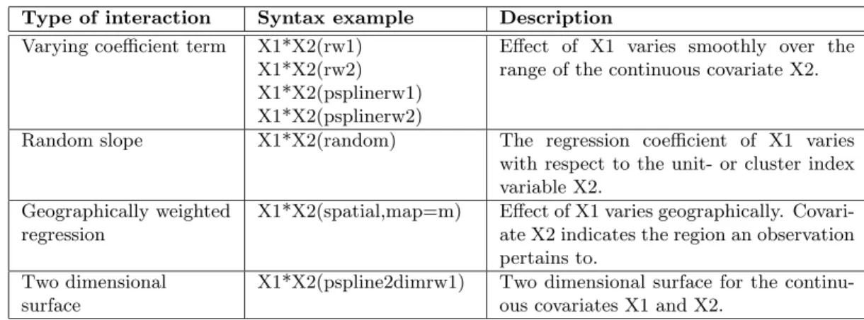
Table 2: Possible interaction terms in BayesX.
Type of interaction Syntax example Description
Varying coefficient term X1*X2(rw1) X1*X2(rw2) X1*X2(psplinerw1) X1*X2(psplinerw2)
Effect of X1 varies smoothly over the range of the continuous covariate X2.
Random slope X1*X2(random) The regression coefficient of X1 varies with respect to the unit- or cluster index variable X2.
Geographically weighted regression
X1*X2(spatial,map=m) Effect of X1 varies geographically. Covari-ate X2 indicCovari-ates the region an observation pertains to.
Two dimensional surface
X1*X2(pspline2dimrw1) Two dimensional surface for the continu-ous covariates X1 and X2.
2.4 graphobjects
graph objects are used to visualize data and estimation results obtained by other objects in BayesX. Currently graph objects may be used to draw scatterplots between variables (method ’plot’), or to draw and color geographical maps stored in map objects (method
’drawmap’). We illustrate the usage of graph objectswith method ’drawmap’ which is used
to color the regions of a map according to some numerical characteristics. The syntax is:
> objectname.drawmap plotvar regionvar [if expression] , map=mapname[options] using
dataset
Method ’drawmap’ draws the map stored in the map object ’mapname’ and prints the graph either on the screen or stores it as a postscript file (if option ’outfile’ is specified). The regions with regioncode ’regionvar’ are colored according to the values of the variable ’plotvar’. The variables ’plotvar’ and ’regionvar’ are supposed to be stored in the dataset object’dataset’. Several options are available for customizing the graph, e.g. for changing from grey scale to color scale or storing the map as a postscript file, see theBayesXmanual Ch. 6. A typical graph obtained with method ’drawmap’ is given in Figure 2.
3
A complex example: Childhood undernutrition in Zambia
In this example we demonstrate the usage ofBayesX by an analysis of data on undernu-trition of children in Zambia. This data set has already been analysed in Kandala et al. (2001). Here, we will use the same model developed in their paper. Since our focus is on demonstrating how a regression model can be specified and estimated using BayesX we do not discuss or interprete the estimation results.Undernutrition among children is usually determined by assessing the anthropometric sta-tus of a child relative to a reference standard. In our example undernutrition is measured through stunting or insufficient height for age, indicating chronic undernutrition. Stunting for a child iis determined using a Z-score which is defined as
Zi = AIi−M AI
σ
Table 3: Response distributions in BayesX.
Family Link Description
gaussian identity Gaussian responses. Details about MCMC inference in Lang and Brezger (2003).
binomial logit Binomial responses. Inference is based on conditional prior or IWLS proposals, see Fahrmeir and Lang (2001a) and Brezger and Lang (2003).
bernoullilogit logit Models with binary responses and logit link. Estimation is based on latent utility representations, see Holmes and Knorr-Held (2003). binomialprobit probit Models with binary responses and probit link. Estimation is based on
latent utility representations, see Albert and Chib (1993). multinomial logit Multinomial logit model, see Brezger and Lang (2003).
multinomialprobit probit Multicategorical probit model. Estimation is based on latent utility representations, see Fahrmeir and Lang (2001b).
cumprobit probit Cumulative threshold model for ordered responses with three cat-egories. Estimation is based on latent utility representations, see Fahrmeir and Lang (2001b).
poisson log Poisson distribution. Inference is based on conditional prior or IWLS proposals, see Fahrmeir and Lang (2001a) and Brezger and Lang (2003).
negbin log Negative Binomial responses. Details in Fahrmeir and Osuna (2003). gamma log Gamma distribution. Inference is based on conditional prior or IWLS proposals, see Fahrmeir and Lang (2001a) and Brezger and Lang (2003).
cox – Cox model. Details in Hennerfeind et al. (2003) and Fahrmeir and Hennerfeind (2003).
example), MAI refers to the median of the reference population andσrefers to the standard deviation of the reference population.
The main interest is on modelling the dependence of undernutrition on covariates including the age of the child, the body mass index of the child‘s mother, the district the child lives in and some further categorial covariates. Table 4 gives a description of the variables used in our model.
The data can be analysed in largely five steps: First we have to read in the data into
BayesX using adataset object. Since we want to estimate a spatial effect of the district in which the child lives, we need the boundaries of the districts to compute the neighbourhood information of the map of Zambia. Therefore, we create a map objectwhich contains the required information in the second step. A regression model is estimated in the third step followed by visualizing results. Since our analysis is based on MCMC-techniques it is important to investigate in a last step the sampling paths and the autocorrelation functions of the estimated parameters.
In the following, we assume that the data set and the map of Zambia are stored in c:\data\zambia.raw and c:\data\mapzambia.raw, respectively.
1. Reading dataset information
To read in the data into BayesXwe create a dataset objectand use theinfilecommand of dataset objects:
> dataset d
Table 4: Variables in the data set on childhood undernutrition.
Variable Description
hazstd Standardised Z-score of stunting.
bmi Body mass index of the mother.
agc Age of the child.
district District where the child lives.
rcw Mother‘s employment status with categories ”working” (= 1) and ”not working” (= −1).
edu1
edu2
Mother‘s educational status with categories ”complete primary but incom-plete secondary” (edu1 = 1), ”complete secondary or higher” (edu2 = 1) and ”no education or incomplete primary” (edu1 =edu2 =−1).
tpr Locality of the domicile with categories ”urban” (= 1) and ”rural” (=−1).
sex Gender of the child with categories ”male” (= 1) and ”female” (= −1).
2. Compute neighbourhood information
The neighbourhood information of the map of Zambia is computed and stored in BayesX
by creating amap objectand using the infilecommand:
> map m
> m.infile using c:\data\mapzambia.raw
Having read in the boundary information, BayesX automatically computes the neigh-bourhood matrix of the map. Two regions are assumed to be neighbours if they share a common boundary.
3. Regression analysis
Now we can estimate our regression model using bayesreg objects. We create a bayesreg objectand estimate the model using the regresscommand:
> bayesreg b
> b.regress hazstd = rcw + edu1 + edu2 + tpr + sex + bmi(psplinerw2) + agc(psplinerw2) + district(spatial,map=m) + district(random), family=gaussian iterations=12000 burnin=2000 step=10 predict using d
The two continuous covariates bmi and agc are assumed to have a possibly nonlinear effect on the Z-score and are therefore modelled by P-splines (with second order random walk penalty). The spatial effect of the district is split up into a spatially correlated effect ’district(spatial,map=m)’ and an uncorrelated effect ’district(random)’, see Fahrmeir and Lang (2001b) for a motivation. The correlated effect is modelled by a Markovrandom field prior. The neighbourhood matrix and possible weights associated with the neighbours are obtained from the map object ’m’.
The options iterations, burninand step define the number of iterations, the burn in period and the thinning parameter. Specifying step=10 as above forces BayesX to store only every 10th sampled parameter which leads to a random sample of length 1000 for every parameter in our example.
If the option predict is specified, samples of the deviance, the effective number of pa-rameters pD and the deviance information criteria DIC of the model are computed and stored, see Spiegelhalter et. al. (2002). In addition, estimates for the additive predictor and the posterior expectation are computed for every observation.
On a 2.4 GHz PC estimation of the model was carried out in about 1 minute and 50 seconds.
After estimation, results for each effect are written to an external ASCII file. These files contain the posterior mean and median, the posterior 2.5%, 10%, 90% and 97.5% quantiles and the corresponding 95% and 80% posterior probabilities of the estimated effects. For example, the beginning of the file for the effect ofbmi looks like this:
intnr bmi pmean pqu2p5 pqu10 pmed pqu90 pqu97p5 pcat95 pcat80 1 12.8 -0.284065 -0.660801 -0.51678 -0.283909 -0.0585753 0.085998 0 -1 2 13.15 -0.276772 -0.609989 -0.483848 -0.275156 -0.070517 0.0572406 0 -1 3 14.01 -0.258674 -0.515628 -0.416837 -0.257793 -0.10009 -0.00289024 -1 -1
The numbers 1 and -1 for the variables pcat95 and pcat80 indicate that the corresponding credible intervals are either strictly positive or negative. Zero indicates credible intervals containing zero.
4. Visualizing estimation results
Estimation results for nonlinear effects ofbmiandagcand the spatial effect of the district are best summarized by visualization. BayesX automatically creates appropriate plots of the effects and stores the graphs as postscript files. The file names are given in the
output window for each effect. Figures 1 and 2 show the content of these files. Moreover, a batch-file is created that contains all commands necessary to reproduce the plots. The advantage is that additional options may be added by the user to customize the graphs (e.g. to change the title or axis labels).
It is also possible to visualize effects on the screen immediatly after estimation. For the nonlinear effects of the two continuous covariates such plots are obtained by executing the commands
> b.plotnonp 1
and
> b.plotnonp 3
The numbers following the plotnonpcommand depend on the order in which the model terms have been specified. The numbers are supplied in the output window after the estimation.
Estimation results for spatial effects are best visualized by drawing the respective map and coloring the regions of the map according to some characteristic of the posterior, e.g. the posterior mean. For instance, the structured spatial effect is visualized by typing
> b.drawmap 5, color
The additional option ’color’ forcesBayesX to use colors instead of grey shades to visu-alize the posterior mean.
5. Post estimation commands
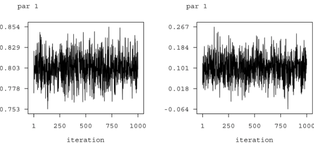
In addition to theregress command,bayesreg objectsprovide some post estimation com-mands to get sampled parameters or to compute autocorrelation functions of sampled parameters. For example
> b.getsample
stores sampled parameters in ASCII files and plots the sampling paths. The resulting graphs are stored in postcript format leading e.g. to the plots shown in Figure 3 for the scale parameter and the intercept. To avoid too large files, the samples are typically partitioned into several files.
Autocorrelation functions may be drawn e.g. by typing
> b.plotautocor , maxlag=150
where ’maxlag’ specifies the maximum lag number. The default is ’maxlag=250’. Execut-ing theplotautocor command also stores the autocorrelation functions in an ASCII file. Figure 4 shows the autocorrelation function for the scale parameter and the intercept.
4
Download and recommendations for further reading
The latest version of BayesXincluding a detailed manual is available athttp://www.stat.uni-muenchen.de/~lang/bayesx/bayesx.html.
The BayesX homepage also contains all files required to produce the results presented in the example on childhood undernutrition in Zambia. In addition, a tutorial based on the Zambia data set is available, click on Tutorials at the homepage. Finally, the boundary and graph files for a number of countries and regions may be downloaded, click on Maps
at the homepage.
If not familar with MCMC simulation techniques, it is strongly recommended to read at least one of the countless introductions into MCMC. A very nice and thorough introduction is given in Green (2001). To get an overview about the methodologyBayesX
is based on, we consider it sufficient to read Chapter 7 of the manual. More details may be found in the references cited in this paper. First steps with BayesXcan be done with the example in this paper and the tutorial on childhood undernutrition in Zambia.
Acknowledgement:
We thank Ludwig Fahrmeir and Andrea Hennerfeind for helpful comments and discus-sions. This research has been financially supported by grants from the German Science Foundation (DFG), Sonderforschungsbereich 386 ”Statistical Analysis of Discrete Struc-tures”.
References
Albert, J. and Chib, S., 1993: Bayesian analysis of binary and polychotomous response data. Journal of the American Statistical Association, 88, 669-679.
Besag, J., York, J. and Mollie, A., 1991: Bayesian image restoration with two applications in spatial statistics (with discussion).Annals of the Institute of Statistical Mathemat-ics, 43, 1-59.
12.8 19.4 26 32.7 39.3 -0.66 -0.36 -0.05 0.26 0.56 Effect of bmi bmi 0 14.8 29.5 44.3 59 -0.28 0.08 0.44 0.8 1.16 Effect of agc agc
Figure 1: Example on childhood undernutrition: Effect of the body mass index of the child‘s mother and of the age of the child together with pointwise 80% and 95% credible intervals.
-0.304985 0 0.22614
Figure 2: Example on childhood undernutrition: Structured spatial effect.
Brezger, A., Kneib, T. and Lang, S., 2003: BayesX manual.
Brezger, A. and Lang, S., 2003: Generalized structured additive regression based on Bayesian P-splines. SFB 386 Discussion paper 321, Department of Statistics, Uni-versity of Munich.
Chen, Z., 1993: Fitting Multivariate Regression Functions by Interaction Spline Models.
Journal of the Royal Statistical Society B, 55, 473-491.
Clayton, D., 1996: Generalized linear mixed models. In: Gilks, W.R., Richardson, S. and Spiegelhalter, D.J.: Markov Chain Monte Carlo in Practice. Chapman and Hall, London.
Fahrmeir, L. and Hennerfeind, A., 2003: Nonparametric Bayesian hazard rate models based on penalized splines. SFB 386 Discussion paper 361, University of Munich. Fahrmeir, L., Kneib, T. and Lang, S., 2003a: Penalized structured additive regression for
space-time data: a Bayesian perspective. SFB 386 Discussion paper 305, University of Munich. Revised forStatistica Sinica.
1 250 500 750 1000 0.753 0.778 0.803 0.829 0.854 iteration par 1 1 250 500 750 1000 -0.064 0.018 0.101 0.184 0.267 iteration par 1
Figure 3: Example on childhood undernutrition: Sampling paths for the scale parameter and the intercept.
1 50 100 150 200 250 0.0 0.2 0.4 0.6 0.8 1.0 lag scale_1_1 1 50 100 150 200 250 0.0 0.2 0.4 0.6 0.8 1.0 lag intercept_1
Figure 4: Example on childhood undernutrition: Autocorrelation functions for the scale parameter and the intercept.
Fahrmeir, L. and Lang, S., 2001a: Bayesian Inference for Generalized Additive Mixed Models Based on MarkovRandom Field Priors.Journal of the Royal Statistical So-ciety C, 50, 201-220.
Fahrmeir, L. and Lang, S., 2001b: Bayesian Semiparametric Regression Analysis of Mul-ticategorical Time-Space Data.Annals of the Institute of Statistical Mathematics, 53, 10-30.
Fahrmeir, L., Lang, S., Wolff, J. and Bender, S., 2003b: Semiparametric Bayesian Time-Space Analysis of Unemployment Duration. Journal of the German Statistical Society, 87, 281-307.
Fahrmeir, L. and Osuna, L. (2003), Structured count data regression. SFB 386 Discussion paper 334, University of Munich.
Fahrmeir, L. and Tutz, G., 2001: Multivariate Statistical Modelling based on Generalized Linear Models, Springer–Verlag, New York.
Fotheringham, A.S., Brunsdon, C., and Charlton, M.E., 2002: Geographically Weighted Regression: The Analysis of Spatially Varying Relationships.Chichester: Wiley.
Fronk, E.–M. and Giudici, P., 2000: MarkovChain Monte Carlo model selection for DAG models. SFB 386 Discussion paper 221, Department of Statistics, University of Munich.
Green, P.J., 2001: A Primer in MarkovChain Monte Carlo. In: Barndorff-Nielsen, O.E., Cox, D.R. and Kl¨uppelberg, C. (eds.), Complex Stochastic Systems. Chapmann and Hall, London, 1-62.
Hastie, T. and Tibshirani, R., 1990: Generalized Additive Models. Chapman and Hall, London.
Hastie, T. and Tibshirani, R., 1993: Varying-coefficient Models. Journal of the Royal Statistical Society B, 55, 757-796.
Hennerfeind, A., Brezger, A. and Fahrmeir, L., 2003: Geoadditive survival models. SFB Discussion paper 333, University of Munich.
Holmes, C.C., and Knorr-Held, L., 2003: Efficient Simulation of Bayesian Logistic Regres-sion Models. DiscusRegres-sion paper 306, SFB 386, Department of Statistics, University of Munich.
Ibrahim, J.G., Chen, M.H. and Sinha, D., 2001: Bayesian Survival Analysis. Springer-Verlag, New YorK.
Kamman, E. E. and Wand, M. P., 2003: Geoadditive Models. Journal of the Royal Sta-tistical Society C, 52, 1-18.
Kandala, N. B., Lang, S., Klasen, S. and Fahrmeir, L., 2001: Semiparametric Analysis of the Socio-Demographic and Spatial Determinants of Undernutrition in Two African Countries. Research in Official Statistics, 1, 81-100.
Lang, S. and Brezger, A., 2003: Bayesian P-splines.Journal of Computational and Graph-ical Statistics, to appear.
Ruppert, D., Wand, M.P. and Carroll, R.J., 2003: Semiparametric Regression.Cambridge University Press.
Spiegelhalter, D.J., Best, N.G., Carlin, B.P. and van der Linde, A. (2002): Bayesian measures of model complexity and fit.Journal of the Royal Statistical Society B, 65, 583 - 639.