water distribution systems
by
Altus Hugo de Klerk
Thesis presented in partial fulfilment of the requirements for the degree Master of Science in Engineering at Stellenbosch University
Supervisor: Prof. H.E. Jacobs Faculty of Engineering Department of Civil Engineering
Division of Water and Environmental Engineering
i
Declaration
By submitting this thesis electronically, I declare that the entirety of the work contained therein is my own, original work, that I am the sole author thereof (save to the extent explicitly
otherwise stated), that reproduction and publication thereof by Stellenbosch University will not infringe any third party rights and that I have not previously in its entirety or in part submitted it for obtaining any qualification.
Copyright © 2016 Stellenbosch University All rights reserved
ii
Abstract
The decision on whether to replace a pipe, with specific reference to a water distribution network, can be complicated by several aspects in the decision making process, such as available funding and required system performance. Long term budget requirements need to be assessed for the effective management of an existing water distribution network to find balance between the return on investment and customer satisfaction.
Various failure prediction models are available to calculate the probability of failure of each pipe in a water network. The probability of failure is then used to determine a replacement priority for all pipes in the network accordingly. Research has shown that the choice and implementation of failure prediction models are sensitive to the availability of data and in many cases a high degree of expertise is required to sufficiently understand the results. Semi-quantitative risk assessments provide a structured way to rank pipes by accounting for likelihood and consequence of failure while providing adaptability to the availability of data. In order to utilise the advantages of the risk-based approach a multi-period replacement model was developed to determine a suitable long term investment strategy, while taking some practical considerations into account.
A model was developed which utilised a risk-based approach to determine the pipe replacement priority. The model considers each pipe in a pipe inventory database based on several contributing pipe attributes and the available budget. A failure forecasting algorithm was also included in the model. The model could be used to determine the required budget based on certain fixed input parameters such as the total length of pipe to be replaced or the total allowed number of failures per year.
Four hypothetical investment scenarios were analysed for a case study. The results were compared to a fifth scenario, noted as the reactive strategy, which involved no pipe replacement. For the specific case study that was analysed the reactive strategy involved the lowest total cumulative expenditure. Additional investment was required to improve the performance indicators for the number of failures, service interruption duration, estimated remaining useful life and estimated remaining asset value. This research presented a methodology across the different performance indicators noted above, wherein the relative weights of the performance indicators were used to calculate a best-fit index.
iii
Opsomming
Die besluit om ‘n pyp te vervang, met spesifieke verwysing na ‘n water verspreidingsnetwerk, kan ingewikkeld wees as gevolg van verskeie aspekte in die besluitnemingsproses, soos beskikbare befondsing en vereistes vir stelsel prestasie. Langtermyn vereistes vir befondsing moet geassesseer word vir die effektiewe bestuur van ‘n bestaande water verspreidingsnetwerk om ‘n balans te vind tussen die opbrengs op belegging en verbruiker tevredenheid.
Verskeie voorspellingsmodelle is beskikbaar om die waarskynlikheid van faling vir elke pyp in die water netwerk te bereken. Die waarskynlikheid van faling word dan gebruik om dienooreenkomstig die prioriteit van vervanging vir alle pype in die netwerk te bepaal. Navorsing toon dat die keuse en uitvoering van voorspellingsmodelle, vir faling, sensitief is ten opsigte van die beskikbare data en in baie gevalle word ‘n hoë graad van kundigheid verlang om die resultate voldoende te verstaan. Semi-kwantitatiewe risiko assesserings bied ‘n gestruktureerde wyse om die pyprang te bepaal deur die waarskynlikheid en gevolge van faling in ag te neem en terselfde tyd aanpasbaarheid tot die beskikbaarheid van data te bied. Ten einde die voordele van die risiko-gebaseerde benadering te gebruik, was ‘n multi-tydperk vervangingsmodel ontwikkel om ‘n geskikte langtermyn beleggingstrategie te bepaal, inaggenome sommige praktiese oorwegings. Die ontwikkelde model het gebruik gemaak van die risiko-gebaseerde benadering om die vervangingsprioriteit van elke pyp te bepaal. Die model neem elke pyp teenwoordig in ‘n pyp inventaris databasis in ag, gebaseer op verskeie bydraende pyp eienskappe en die beskikbare begroting. ‘n Algoritme vir die vooruitskatting van falings was ook by die model ingesluit. Die model kan gebruik word om die benodigde begroting te bepaal gebaseer op sekere vaste inset parameters soos die totale lengte pyp wat vervang moet word of die totale aantal falings wat toegelaat word per jaar.
Vier hipotetiese belegging scenarios was geanaliseer vir ‘n gevallestudie. Die resultate was dan vergelyk met ‘n vyfde scenario, bekend as die reaktiewe strategie, waar geen pyp vervanging plaasgevind het nie. Vir die spesifieke geanaliseerde gevallestudie het die reaktiewe strategie die laagste kumulatiewe uitgawes getoon. Addisionele belegging was benodig om die prestasie-aanwysers vir die aantal falings, diens onderbrekingsduur, geskatte nuttige oorblywende lewensduur en verwagte oorblywende batewaarde. Hierdie navorsing het ‘n metode aangebied waar die relatiewe gewig toegeken aan die verskeie prestasie-aanwysers, soos hierbo genoem, gebruik word om ‘n beste-pas indeks te bereken.
iv
Acknowledgements
I acknowledge my employer, GLS Consulting, for affording me the opportunity to pursue my Master’s degree. A special thanks to Dr. Leon Geustyn, Dr. Alex Sinske and Adrian van Heerden for their suggestions and support.
I would like to thank my supervisor Prof. Heinz Jacobs for his guidance during the development of this thesis.
Finally, I want to thank my family and friends who stood by me and always believed in me, even in the times when I did not do so myself.
v
Table of Contents
Declaration ... i Abstract ... ii Opsomming ... iii Acknowledgements ... iv Table of Contents ... vList of Equations ... vii
List of Figures ... viii
List of Tables ... x
List of abbreviations and acronyms ... xii
List of symbols ... xiv
1 Introduction ... 1 1.1 Background ... 1 1.2 Terminology ... 2 1.3 Research context ... 5 1.4 Problem statement ... 6 1.5 Research objectives ... 7
1.6 Description of case study ... 8
1.7 Research methodology ... 8
1.8 Scope and limitations ... 10
2 Literature Review ... 12
2.1 Water distribution network layout ... 12
2.2 Pipe deterioration process ... 13
2.3 Pipe failure modes ... 13
2.4 Factors contributing to pipe failure ... 15
2.5 Consequence of failure ... 20
2.6 Failure prediction models ... 23
vi
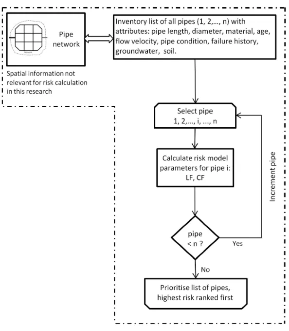
3 Description of the once-off risk prioritisation approach ... 34
3.1 Risk model framework ... 34
3.2 Risk calculation ... 35
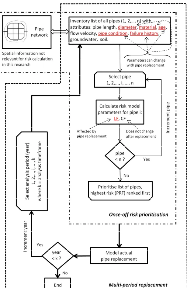
4 Development of the multi-period prioritisation model (MPM) ... 38
4.1 MPM framework ... 38
4.2 Key model concepts ... 40
4.3 Mathematical description ... 46
4.4 Description of MPM tool ... 57
5 Illustration of model application to a water distribution system ... 67
5.1 Case study available data ... 67
5.2 Model robustness tests ... 78
5.3 Validation of risk-based replacement ... 95
5.4 Investment strategy comparison for case study ... 101
6 Conclusion ... 113
6.1 Findings from literature ... 113
6.2 MPM tool ... 113
6.3 Future investigation and improvements ... 115
7 Reference List ... 117 Appendix A: MPM process steps... I Appendix B: Robustness test results ... VI Appendix C: Validation test results ... XXIV Appendix D: Investment scenario results ... XXXVII Appendix E: Best-fit solution comparisons ... XLVIII
vii
List of Equations
Equation 1: Likelihood of failure (adapted from Sinske et al., 2011)... 35
Equation 2: Consequence of failure (adapted from Sinske et al., 2011) ... 36
Equation 3: Pipe replacement factor (adapted from Sinske et al., 2011) ... 37
Equation 4: Unit replacement cost ... 47
Equation 5: Unit repair cost ... 47
Equation 6: Time-exponential failure rate increase (Shamir and Howard, 1979) ... 47
Equation 7: Alteration to the time-exponential failure rate increase equation... 49
Equation 8: Frailty factor ... 50
Equation 9: Initial failure calculation... 51
Equation 10: Correction factor per diameter group ... 52
Equation 11: Expected number of failures for pipe in analysis period ... 52
Equation 12: Replacement time ... 53
Equation 13: Repair time ... 53
Equation 14: Planned SID ... 54
Equation 15: Unplanned SID ... 54
Equation 16: Cumulative expenditure... 55
Equation 17: Operational expenditure ... 55
viii
List of Figures
Figure 1-1: Schematic research methodology ... 9
Figure 2-1: Typical water distribution network layout ... 12
Figure 2-2: Multi-step pipe failure process (Misiunas, 2005) ... 13
Figure 2-3: Hypothetical failure rate of water pipe over service life ... 17
Figure 2-4: Installation periods per material (adapted from Mora-Rodriguez et al., 2014) ... 18
Figure 2-5: Direct costs due to a failure over time (adapted from Misiunas, 2005) ... 21
Figure 2-6: Direct and indirect cost of failure (adapted from Misiunas, 2005) ... 22
Figure 3-1: Once-off risk prioritisation framework ... 34
Figure 4-1: Multi-period replacement model framework ... 39
Figure 4-2: MPM process ... 58
Figure 4-3: Pre-processing procedure workflow ... 59
Figure 4-4: Example of "OUTPUT" sheet with results ... 65
Figure 4-5: Example of "STATS" sheet with results ... 66
Figure 5-1: Percentage of total length per diameter range ... 68
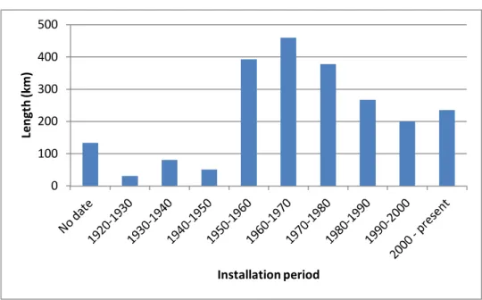
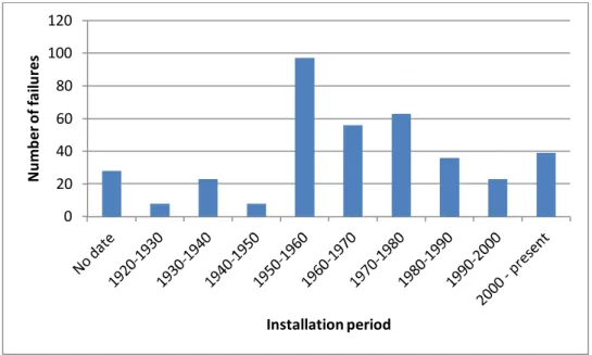
Figure 5-2: Length of pipe per installation period ... 69
Figure 5-3: Number of recorded failures per installation period ... 70
Figure 5-4: Failures per 100km per installation period ... 70
Figure 5-5: Percentage of total length per material ... 71
Figure 5-6: Number of failures per 100km per material ... 72
Figure 5-7: Distribution of ERUL per material ... 73
Figure 5-8: Increase in exponential factor per material ... 77
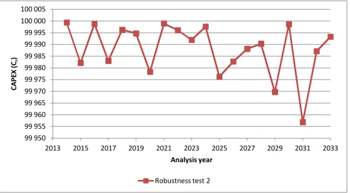
Figure 5-9: CAPEX for Robustness test 2 ... 81
Figure 5-10: Comparison of number of failures between Robustness tests 1 and 2 ... 82
Figure 5-11: Comparison of ERAV between Robustness tests 1 and 2 ... 82
Figure 5-12: Replaced length for Robustness test 3 ... 83
Figure 5-13: Comparison of planned SID between Robustness tests 2 and 4 ... 84
Figure 5-14: Total number of failures for Robustness test 5 ... 85
Figure 5-15: CAPEX for Robustness test 5 (required AARB to restrict failures) ... 85
Figure 5-16: CAPEX for Robustness test 6 ... 86
Figure 5-17: CAPEX based on pipe skip count parameter for Robustness test 7 ... 88
Figure 5-18: Comparison of number of failures for Robustness tests 1 and 9 ... 90
Figure 5-19: Comparison of total number of failures on AC pipes ... 91
Figure 5-20: Comparison of total number of failures on PVC pipes ... 91
ix
Figure 5-22: Random replacement - Failures predicted ... 96
Figure 5-23: Random replacement - Total SID ... 97
Figure 5-24: Random replacement - Average network ERUL ... 97
Figure 5-25: Age-based replacement - Failures predicted ... 98
Figure 5-26: Age-based replacement - Total SID ... 98
Figure 5-27: Age-based replacement - Average network ERUL ... 99
Figure 5-28: ERUL-based replacement - Failures predicted ... 100
Figure 5-29: ERUL-based replacement - Total SID ... 100
Figure 5-30: ERUL-based replacement - Average network ERUL ... 101
Figure 5-31: Comparison of annual CAPEX for investment scenarios ... 103
Figure 5-32: Comparison of annual number of failures for investment scenarios ... 104
Figure 5-33: Comparison of annual OPEX for investment scenarios ... 105
Figure 5-34: Comparison of annual total SID for investment scenarios ... 106
Figure 5-35: Comparison of annual ERAV for investment scenarios ... 106
Figure 5-36: Comparison of TCE for investment scenarios ... 107
Figure 5-37: Comparison of the difference in ERAV and TCE for investment scenarios ... 108
Figure 5-38: Comparison of annual average network ERUL for investment scenarios ... 108
Figure 5-39: Comparison of cumulative replacement length as percentage of total length ... 109
Figure 5-40: Calculation of TCE index... 110
x
List of Tables
Table 2-1: Failure modes in water pipes (NGSMI, 2003) ... 14
Table 2-2: Physical factors contributing to failure in water pipes (adapted from NGSMI, 2003; USEPA, 2000; Wood and Lence, 2009) ... 15
Table 2-3: Environmental factors contributing to failure in water pipes (adapted from NGSMI, 2003; USEPA, 2000; Wood and Lence, 2009) ... 16
Table 2-4: Operational factors contributing to failure in water pipes (adapted from NGSMI, 2003; USEPA, 2000; Wood and Lence, 2009) ... 16
Table 2-5: Time-relationship models ... 24
Table 2-6: Failure clustering models ... 26
Table 2-7: Probabilistic and statistical models ... 27
Table 2-8: Bayesian models ... 29
Table 2-9: Advanced mathematical models ... 30
Table 2-10: Summary of risk assessment categories ... 32
Table 3-1: Likelihood variables for case study ... 36
Table 3-2: Consequence variables for case study ... 36
Table 4-1: Replacement cost function ... 41
Table 4-2: Repair cost function ... 45
Table 4-3: Sheet layout for MPM tool ... 57
Table 4-4: Minimum required data ... 60
Table 4-5: Pipe Material Life input table ... 61
Table 4-6: Diameter grouping and replacement ... 62
Table 4-7: Example of Likelihood score rating legend ... 63
Table 4-8: Example of Likelihood factor weight assignment ... 63
Table 4-9: Input sheet options ... 64
Table 5-1: Length and failures per diameter range ... 68
Table 5-2: Length and failure per material ... 71
Table 5-3: Estimated service life ... 73
Table 5-4: Interruption due to repairs (min/failure) ... 74
Table 5-5: Interruption due to replacements ... 74
Table 5-6: Likelihood of failure score assignment ... 75
Table 5-7: Likelihood of failure weight assignment ... 76
Table 5-8: Pipe material replacement and grouping ... 76
Table 5-9: Failure growth rate coefficients (Neelakantan et al., 2008) ... 77
xi
Table 5-11: Summary of robustness tests for MPM model ... 79
Table 5-12: Correction factor per diameter group for robustness tests ... 80
Table 5-13: Comparison of failures for Robustness test 1 ... 81
Table 5-14: CAPEX with pipe skip count parameters for Robustness test 7... 87
Table 5-15: CAPEX with contingency buffer for Robustness test 8 ... 89
Table 5-16: Comparison of AM for Robustness test 9 and. Robustness test 1 ... 90
Table 5-17: Recurring replacement as percentage of replaced length for Robustness test 10 ... 92
Table 5-18: CAPEX breakdown for Robustness test 11 ... 94
Table 5-19: Summary of validation scenarios ... 95
Table 5-20: Base failure input per diameter group ... 101
Table 5-21: Summary of investment scenarios ... 102
Table 5-22: Comparison of TCE with reactive strategy ... 110
Table 5-23: Weighting scheme examples for comparison of best-fit solution ... 111
Table 5-24: Best-fit solution - weighting scheme 1 ... 112
Table 5-25: Best-fit solution - weighting scheme 2 ... 112
xii
List of abbreviations and acronyms
AARB Available Annual Replacement BudgetAC Asbestos Cement
ALM Accelerated Lifetime Model ANN Artificial Neural Networks
AMP Asset Management Plan
CAPEX Capital Expenditure
CF Consequence of Failure
CI Cast Iron
DI Ductile Iron
DSS Decision Support Systems
ERAV Estimated Remaining Asset Value ERUL Estimated Remaining Useful Life ESL Estimated service life
GIS Geographic Information System
GWL Ground Water Level
HDPE High Density Polyethylene
ID Identification
km kilometre
KPI Key Performance Indicator
LF Likelihood of Failure
m metre
xiii MPM Multi-period Prioritisation Model
NGSMI National Guide to Sustainable Municipal Infrastructure OPEX Operational Expenditure
PE Polyethylene
PHM Proportional Hazard Model
PI Performance Indicator
pH Decimal co-logarithm of Hydrogen
PRF Pipe Replacement Factor
PVC Polyvinyl Chloride
REP Replacement exclusion period
RUL Remaining Useful Life
SID Service interruption duration
ST Steel
TCE Total Cumulative Expenditure
xiv
List of symbols
ϴi LF variable weight
ϴT Total of all LF variable weights
LF variable score
фT Total of all CF variable weights
фj CF variable weight
CF variable score
Unit replacement cost per unit length Unit repair cost per failure
Number of failures
() Failure rate in analysis period t
( ) Failure rate at start of the analysis A Growth rate coefficient
Np(t) Failure rate in analysis period t for pipe
Nd,p(t0) Failure rate at start of the analysis for diameter group of pipe
AM,p Growth rate coefficient for material of pipe
t Analysis period (typically year) t0 Initial or starting period
ap Age of pipe
Frailty factor for pipe
Fp(t0) Calculated failures for pipe at start of analysis
CFd Diameter group correction factor
xv Fd Total initial failures for diameter group
Fp(t) Expected failures for pipe in analysis period
Tp Replacement time
Tu Repair time
SIDp Planned service interruption duration
Tp,i Time for replacement of pipe selected for replacement
HHi Number of affected users (households)
TH Total number of affected users (households) in the system SIDu Unplanned service interruption duration
Tu,i Time for repair of pipe
CEi Cumulative expenditure if pipe is replaced
CEi-1 Cumulative expenditure before current pipe is considered
, Estimated remaining useful life of pipe, given pipe material and age EM,i Estimated service life of pipe material
1
1
Introduction
1.1
Background
The world is undergoing the largest wave of urban growth in history due to the combined effect of urbanisation and population increase (UNFPA, 2014). Additional system load places an extra burden on relatively old established water distribution networks. The effective management of operational infrastructure could result in increased asset life and would subsequently reduce the required replacement of ageing components. Therefore, the effective management of water distribution network infrastructure is of great importance to ensure the sustainable delivery of water services.
Minnaar et al. (2013) stated that asset management is an important part of any organisation as it allows them to extract value from their assets and further that municipal managers are under increasing pressure to adopt an asset management plan (AMP). The ISO 55000 series of international standards provide a universally applicable set of asset management principles. An AMP involves reporting on the status of the system, on a component level according to certain criteria.
It was reported in the National Guide to Sustainable Municipal Infrastructure (NGSMI) (2003) that urban water infrastructure is deteriorating at a higher rate than the renewal rate due to various factors such as low funding, inadequate inspection, poor quality control and lack of consistency in operation practices. Pelletier et al. (2003) state that water distribution pipes are among the infrastructure that is deteriorating and that municipal water managers attribute the deterioration to the lack of investment in proactive replacement and refurbishment programmes. Effective management of operational infrastructure is required to ensure sustainable water service delivery. The majority of water distribution network’s infrastructure components consist of pipes and generally represent a large proportion of the asset value and therefore their management is an important issue. Pipes have a certain expected asset life, associated with the material of the pipe necessitating replacement with a similar or improved pipe at some estimated future date.
The replacement of pipes, damaged and otherwise affected, is an integral part in the effective management of a water distribution network. Decisions on replacement or rehabilitation are made based on a perceived risk of failure, which is a combination of the probability of an asset failure occurring and the consequence of said failure. Asset condition is used to determine the risk of failure and remaining useful life, but conducting condition assessments on buried infrastructure is relatively complicated.
2
The probability of pipe failure is required for effective management and risk calculation. Therefore, records are required of pipe assets and subsequent failure data covering each asset’s lifetime. Some challenges faced by municipalities for pipe failure data collection include limited personnel and resources, missing or incomplete historical data, conflicting data and non-computerised information in combination with the retirement of staff who hold such tacit knowledge (Pelletier, 2003; Wood et al., 2007). According to Wood and Lence (2006), data collection involves direct financial costs which present a serious constraint for municipalities with limited budgets.
Ganguly and Gupta (2004) stated that the techniques in sophisticated decision support systems (DSS) are computationally intense, but that with the continuous advancements in computing technologies and processing speeds the implementation of such systems are expected to become more commonplace. However, as stated by Zopounidis and Doumpos (2008), much insight is required to confidently apply the obtained results in the decision-making process as the decision makers themselves need to examine the obtained results to determine to the most appropriate decision. Clair and Sinha (2012) mention that many of the predictive models found in literature are relatively complicated for the average municipality to apply to their own water infrastructure.
Risk-based asset prioritisation is attaining popularity as a tool to manage assets comprehensively (Park et al., 2010) and is effective for management of pipe replacement programmes (Shaikh, 2010). Risk-based prioritisation accounts for factors that influence pipe failure, consequence of failure and management strategies. In other words, preference could be given to replace asbestos-cement (AC) pipes due to possible health risks, regardless of remaining useful life. A priority can be assigned to each pipe asset and appropriate decisions made on replacement and rehabilitation programmes.
1.2
Terminology
The terms defined below are used with their stated meaning in this research to avoid confusion as some studies use different terms to describe similar concepts.
Consequence of failure: The definition for “consequence of failure” as provided by Park et al. (2010), namely “the consequence of physical failure of a component is a measure of the impact on the community and customers”, was adopted for this research.
3
Estimated service life: The actual service life of a pipe is not known until failure occurs. Fisher (2008) stated that when deciding which material to use the life expectancy of the asset is fundamental. In this research, the “estimated service life” of a pipe is based on the material and can be obtained from a supplier catalogue or substituted with a subjective value from engineering knowledge.
Estimated remaining useful life: Sinske et al. (2009) calculated the remaining useful life by subtracting the actual age of the pipe from the life expectancy based on the pipe material. Sinske and Streicher (2013) adopted the same calculation; however the term “remaining useful life” was substituted with the more descriptive term, “catalogue remaining useful life”, in order to indicate that standard expected useful life was retrieved from a supplier catalogue. Analogously to the latter, in this research, the term “estimated remaining useful life” is used, in order to indicate that the estimated service life is used to approximate the useful life of the pipe.
Failure: The term “failure” is used as described by De Oliveira et al. (2011), who stated that a failure is a set of events which are detected by the municipality and required a repair or replacement activity for which a maintenance record was issued. A failure typically results in the loss of water and might include pipe bursts and leakage, depending on how the failure records for the municipality are stored. Some authors use the term “break”, in which case reference should be made to the original source to clarify the meaning.
Failure rate: The term “break rate” or “breakage rate” was widely used in analyses of pipe failures in water distribution networks (Walski and Pelleccia, 1982; Rostum, 2000; Wood and Lence, 2009). Misiunas (2005) uses the term failure frequency while others (Achim et al., 2007; Martins, 2013) use the term failure rate. In this research the term “failure rate” is used, except when in reference to studies performed by other authors. The failure rate for a given pipe or set of pipes are generally normalised on length and time (Rostum, 2000) and expressed as the number of failures per length per time. In this research the failure rate is expressed as the annual number of failures per 100km as suggested by Lambert and Taylor (2010). In this text, the unit will be expressed as (
∙ ).
Likelihood of failure: The likelihood of failure is an indication of the probability of a failure occurring and is often expressed as the expected value from the probability distributions in statistical or stochastic failure prediction models (Loganthan et al., 2002; Vanrenterghem-Raven, 2007; Martins, 2011). In this research, the likelihood of failure is treated analogously to that of consequence of failure whereby it represents a measure of the expected influence of a pipe attribute and its value on the possible failure of a pipe.
4
Pipe: A pipe represents the concatenation of individual pipe entities with similar characteristics. Pipe nodes act as separators to split the pipes at intersection of pipes with different characteristics (De Oliveira et al., 2011). The term pipe was similarly described by Rostum (2000) as consisting of many segments or lengths “from one node in the water network to another” (for example, a change in material) and typically with a length of between 50m and 150m. For this research a pipe will be subject to the pipe inventory database used and each record will denote a single pipe. When presenting the model (chapter 3 and 4) the total number of pipes in the database is denoted by the parameter n (always an integer).
Pipe age: In this research, the pipe age refers to the time, in years, that the pipe has been in operation and is calculated as the difference in years from the installation year of the pipe to the analysis year as applicable in the model.
Proactive strategy: The term “proactive maintenance” was described by Arsénio (2013) to be any maintenance activity that is performed to delay deterioration or failure of a component or system; Rostum (2000) stated that a strategy is deemed to be proactive in water network management if replacement or repair activities were taken prior to a failure event. In this research, any investment scenario, with an available replacement budget greater than zero, is deemed to be a proactive strategy because it will result in the replacement of a pipe before a known failure. Reactive strategy: The term “reactive maintenance” was described by Arsénio (2013) to be any maintenance activity that is performed after a failure to repair damage or restore infrastructure to satisfactory operational levels; Rostum (2000) stated that a strategy is deemed to be reactive in water network management if replacement or repair action is taken after a failure event occurs. In this research, a reactive strategy is one where the available replacement budget is equal zero, because it will result in no replacement activity.
Repair: The terminology of Rostum (2000) was used to describe a repair as follows, “An unplanned maintenance activity carried out after the occurrence of a failure”.
Repair time: Walski and Pelleccia (1982) indicated that the time to isolate the system and perform the repair activities depend on several factors and calculated the time in hours. In this research the repair time does not only refer to the time of repair, but is normalised by taking into account the number of consumers (households) affected by the failure and the total number of consumers in the system to compare the severity or impact of each failure in terms of the interruption in service.
5
Replacement: Rostum (2000) defined replacement as the “construction of a new pipe, on or off the line of an existing pipe” and also that “the function of the pipe will incorporate that of the old, but may also include improvements”. In this research a replacement will be on the line of the existing pipe that is being replaced and also will not offer any improvements, that is, the hydraulics of the distribution network are the same as before the replacement occurred.
Replacement cost: Investopedia (2015) defines replacement cost as “the price that will have to be paid to replace an existing asset with a similar asset” and Johnstone (2003) mentioned that research has shown that regulators find current replacement cost to be the most appropriate valuation basis. The terminology of RAMM (2011) was used to describe the replacement cost as “a form of asset valuation where cost of replacing a pipe is determined by calculating the current cost of the most appropriate modern asset with equivalent service potential”.
Replacement time: Similar to the repair time, the replacement time is the time for the replacement activity, the time from when the replaced pipe is taken out of service to the time the new pipe is in operation, which is then normalised by number of households to compare the replacement impact in terms of the interruption in service.
Service life: According to ISO Standard 15686 defined as “The period of time after installation during which a building or its parts meet or exceed the performance requirements”. The same definition can be applied for water distribution networks, namely “The period of time after installation during which a water distribution network or its parts meet or exceed the performance requirements”. In this research, the parts of the water distribution network that are considered are the reticulation pipes.
Service interruption duration: Stacha (1978) commented on the importance of service continuity to minimise customer inconvenience and provided a cost table in an attempt to quantify the cost of interruptions due to pipe failures. In this research, the inconvenience of pipe failure is measured as the expected interruption in water supply to customers due to replacement or repair operations and is expressed as the cumulative minutes of interruption for affected consumers divided by the total number of consumers in the system. The service interruption duration may also be colloquially referred to as “downtime”.
1.3
Research context
Renaud et al. (2011) stated that buried water pipe networks represent “more than 80% of the total asset value for water distribution systems”; the effective management of pipe networks is essential. Wood and Lence (2006) suggested that DSS tools for prioritising the replacement or
6
rehabilitation of water mains should be tailored according to the quality of data available to a municipality; and municipalities with minimal or incomplete data cannot use sophisticated tools such as physical or statistical pipe deterioration models and life-cycle costing. Matthews et al. (2012) noted that municipalities required DSS tools to be user-friendly and that minor training should be required to minimise the learning curve.
Wood and Lence (2006) point out that development of robust approaches are required for municipalities with minimal data records. In the South African context, the principle of a user-friendly tool that requires only minor training is of great importance. Lawless (2006) reported that 79 of South Africa’s 231 local municipalities did not employ an engineer, technologist or technician.
Grigg et al. (2013) mentioned that water distribution pipe replacement planning takes place within the sphere of an asset management programme and also noted the requirement of risk assessments to identify the replacement projects that are most critical in order to wisely allocate available resources. Misiunas (2005) indicated that high costs and the slow inspection speeds were a hindrance for the extensive application of many condition assessment techniques in water distribution networks. Giustolisi et al. (2006) stated that municipal water managers need reliable plans for the replacement of critical pipes while weighing up expected benefits against investment in risk-based management scenarios. Rosness (1998) noted that the accuracy of risk analyses depend for the most part on analyst competence and their ability to integrate their own knowledge and assumptions with a critical evaluation of the information.
Crigg et al. (2013) found that the ability to predict failures in a water distribution network was poor and it is with cognisance of the poor ability to predict failures that the usefulness of risk-based prioritisation for water distribution pipe replacement comes to the fore. However, as validation, a multi-period assessment is required to determine whether the replacement based on the calculated risks are sensible, and furthermore to determine whether proposed capital investments are at an acceptable level for ensuring a sustainable water supply while providing the municipality with an indication of whether the available budget is sufficient to manage the water pipe infrastructure.
1.4
Problem statement
Lambert (2012) indicates that the purpose of a water distribution network is to deliver high quality potable water to customers and that throughout the world these networks are getting older and deteriorating. The ageing infrastructure, in combination with higher water demands from urban growth, increase the strain on the water distribution networks and can lead to a higher
7
number of pipe failures. Financial constraints are an obstruction encountered by most municipalities and a balance between proactive assessment and reactive refurbishment is required for optimal use of assigned or available budgets.
Risk-based prioritisation is an effective and proactive way to manage pipe replacement programmes. Shaikh (2010) noted that a risk-based management approach is particularly beneficial to municipalities on a limited budget because it provides municipal managers with an insight into future budget requirements. It is therefore required to expand the useful risk-based prioritisation approach into a multi-period model to provide insight into required replacement budgets and strategies to be employed, measured against certain performance indicators (PI).
1.5
Research objectives
The aim of this research is to expand a once-off pipe risk prioritisation analysis in water distribution systems into a multi-period replacement model that can aid in decision-making processes aimed at determining the required budgets for replacement and refurbishment projects of a municipality. An algorithm was developed to estimate the number of pipe failures in a water distribution system in order to test the effectiveness of pipe replacement options and to estimate the required budget for refurbishment costs and unplanned interruption to service.
The following research objectives were set for this research:
· Provide a literature review on factors that lead to pipe failures and available water pipe failure prediction models.
· Provide a description of the risk-based prioritisation model as implemented for the case study.
· Establish a multi-period risk-based replacement analysis methodology, utilising an annual pipe replacement budget and other practical operational limitation inputs for replacement eligibility testing.
· Determine a suitable failure forecasting algorithm that incorporates the variables used for the calculation of the likelihood of failure in the risk model.
· Illustrate validation and practical application of the model by considering a case study with various input scenarios.
8
1.6
Description of case study
In order to verify the functionality of the developed model, the implementation of a case study was conducted to illustrate the practical application. The case study chosen was for water pipe assets for which a “once-off” risk-based prioritisation was performed by the author as part of a separate investigation. The input parameters and results of the “once-off” prioritisation were used as the base data input for the multi-period analysis.
The name of the water utility was not disclosed in this text for reasons of confidentiality. The region served comprised a total land area of approximately 885,89 km2 and is located in central Europe. The case study dataset has n = 32 957 pipes with a combined length of 2 229,37 km. The service area includes approximately 31 832 rural and 83 168 urban consumers (households). The reason for the choice of this case study data is the low number of annual failures recorded, amounting to a failure rate of approximately .
∙ ; even with long-term failure records the low failure rate would make the use of alternative statistical or probabilistic models difficult to employ, due to the low confidence the predictions would yield.
The utility that is managing the water infrastructure in the case study area places emphasis on consumer satisfaction, which means that data on interruption duration is available and could therefore be calculated for use as a PI in the analysis.
1.7
Research methodology
Kothari (2004) noted that research can either be classified as applied research or fundamental research. Roll-Hansen (2009) stated that applied research is dedicated to the solution of practical economic, social and political problems and although such research depends on scientific knowledge and methods, applied research does not aim at further development of such knowledge and methods. Rajasekar et al. (2013) defines basic (fundamental) research as “an investigation on basic principles and reasons for occurrence of a particular event or process or phenomenon”, and further stated that although basic research is not concerned with solving practical problems, the outcomes from such research are required for any applied research. In this applied research project the feasiblity of utilising risk-based prioritisation in a multi-period replacement model, to aid in the determination of required budgets for pipe replacement projects, was explored. Basic research was conducted as part of the process to investigate the factors that influence the failure of pipes in a water distribution network.
9
A quantitative-simulation research approach was used for the development of a multi-period replacement model. Rajasekar et al. (2013) stated that the charachteristics of a quantitative approach are:
· the approach is numerical and applies statistics or mathematics and uses numbers. · the process is iterative whereby evidence is evaluated.
· the results are often presented in tables and graphs. · the what, where and when of decision making.
According to Kothari (2004), the simulation approach is a sub-class of the quantitative approach which involves the construction of an artificial environment whithin which relevant data can be generated. The term ‘simulation’ referes to the operation of a numerical model that represents the structure of a dynamic process. Given a set of initial variables, a simulation is run to represent the behaviour of the process over time and can be useful in constructing models for the understanding of future conditions.
The development of a numerical model to simulate the replacement process over an extended time period was required. The simulation analysis was performed on secondary data, meaning that the data as collected and available for the case study was used in this research. Figure 1-1 illustrates the approach followed in this research to accomplish the objectives as set out.
10
1.8
Scope and limitations
This research focused on expanding an existing method for risk-based prioritisation. For this research it was accepted that the scores and weights of the various factors influencing the likelihood of failure, as well as those of the consequence of failure, have been established beforehand. In other words this research excluded hydraulic network modelling – the outputs of a hydraulic model for the case study concerned (for example flow rate and pressure) were used as some of the inputs in deriving the risk model presented in this research. Therefore, this research explored the expansion of the risk-based method, as employed by the case study presented, into a multi-period analysis. For this research, a time step period of one year was considered. The corresponding failure estimation algorithms are therefore based on a period of one year.
The model was limited to distinguish between the failure rates for a maximum of three pipe diameter groups. The diameter groups considered during this research were: small, medium and large pipes, based on a suitable diameter range as discussed later in the text.
The input parameters as available for the case study were used for the calculation of replacement and repair time to determine the service interruption duration (SID). Verification of the provided interruption statistics against other data was beyond the scope of this research.
Six replacement cost functions were provided for in this research. Cost functions were available for three replacement pipe material categories, namely Polyvinyl Chloride (PVC), Ductile Iron (DI) and Polyethylene (PE). Each of the three material categories is duplicated within the two location identifiers, i.e. urban or rural, and presented in tabular form for discrete pipe diameter ranges. Also important to note is that the cost functions used to determine replacement value are based on open-trench excavations; trenchless technologies were excluded. The replacement cost functions are limited to the three distinct material categories. A length-weighted average cost was calculated for substitution for other materials in the network.
The effects of replacement on a non-expanding water distribution network were considered. In other words, alterations and additions to the pipes in the water distribution network, beyond changes to material, installation date, pipe condition and failure history, were not considered as part of this research. The assumption of a static network (non-expanding) was considered reasonable for the case study as it is situated in central Europe, where many towns have not grown substantially and rather tend toward densification.
The developed tool only allows for one decision, namely whether to replace the pipe asset or not. Pipes eligible for replacement in a given period would thus be replaced. No allowance was made
11
for further decision-tree branches such as the choice between replacement, refurbishment or condition inspection. For the analysis and verification process, it was deemed satisfactory to assume that all costs would increase at the same rate so as to compare annual incurred costs in terms of present value. Applying a discount rate to calculate the net present value as eligibility test was thus not required.
The Local Government Capital Asset Management Guideline of the Municipal Finance Management Act (2008) stated that the most common depreciation methods that can be applied are the (i) straight line, (ii) diminishing balance and (iii) sum of units depreciation methods, and further stated that National Treasury recommends the straight line method. Accordingly, the pipe asset value was calculated based on a linear depreciation function which accounted for the current replacement cost and the expected service life of the pipe material. No other depreciation models were considered for this research as Hosking and Jacoby (2013) found that the majority of the municipalities included in their research used the straight line depreciation method as recommended by National Treasury.
12
2
Literature Review
2.1
Water distribution network layout
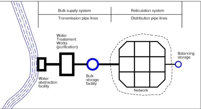
Misiunas (2005) stated that the objectives of an urban water supply system are to provide safe, potable water to consumers, and adequate water at sufficient pressure for fire protection. The layout of a water distribution network is illustrated in Figure 2-1. The network can be divided into abstraction, treatment, storage and distribution components.
Figure 2-1: Typical water distribution network layout
Shamsi (2002) states that the bulk of a distribution network’s infrastructure components consist of pipe assets. Al-Barqawi and Zayed (2006) stated that a water delivery system can be grouped into two categories: transmission and distribution systems (locally the terms bulk and reticulation are more common). Water is transferred from the main source to the storage system via transmission pipes or so-called bulk system pipes. Distribution pipes (reticulation pipes) convey water from the point of storage to the end-user. The focus of this research is on the distribution network pipelines, shown inside the dotted circle in Figure 2-1.
De Oliveira et al. (2011) stated that the usual portrayal of a distribution network is “a planar graph in which edges represent pipes and nodes represent pipe intersections”. In the interest of simplification, pipes represent the concatenation of individual pipe entities with similar characteristics. Pipe nodes act as separators to split the pipes at the intersection of pipes with different characteristics.
13
Poulton et al. (2007) also stated that pipes records in a geographical information system (GIS) result from the splitting of long pipes into shorter sections due to various practical considerations, most notably for the purpose of hydraulic analyses, where additional pipe nodes may be required for a better spatial representation of the demand in the distribution network.
2.2
Pipe deterioration process
A multi-step process as provided by Misiunas (2005) to describe pipe failure is shown in Figure 2-2. Makar and Kleiner (2000) reported that the failure rate of pipes is a function of pipe material, operational conditions and exposure to undesirable environmental factors. Al-Barqawi and Zayed (2006) noted that deterioration varies from one distribution network to another, because these processes are based on different uncertain factors affecting the condition level.
Figure 2-2: Multi-step pipe failure process (Misiunas, 2005)
Kleiner and Rajani (2002) provided the following classification for deterioration factors:
· Static factors relating to pipe attributes remain relatively constant and include material, length and diameter.
· Dynamic factors relating to pipe environment and other factors that change over time and include age, corrosive factors and dynamic loadings such as traffic.
· Operational factors relating to replacement rates, protection methods and water pressures.
2.3
Pipe failure modes
Failure occurs in a water pipe when the extent of degradation has progressed sufficiently so that a pipe can no longer withstand the forces acting on it. Wood et al. (2007) reported that the type of pipe failure could not be correlated to a specific cause of failure, but that data on the type of failure could indicate a failure mechanism. In their assessment, Wood et al. (2007) also found that due to pipe failures being treated reactively as emergencies, and staff on site focusing on
14
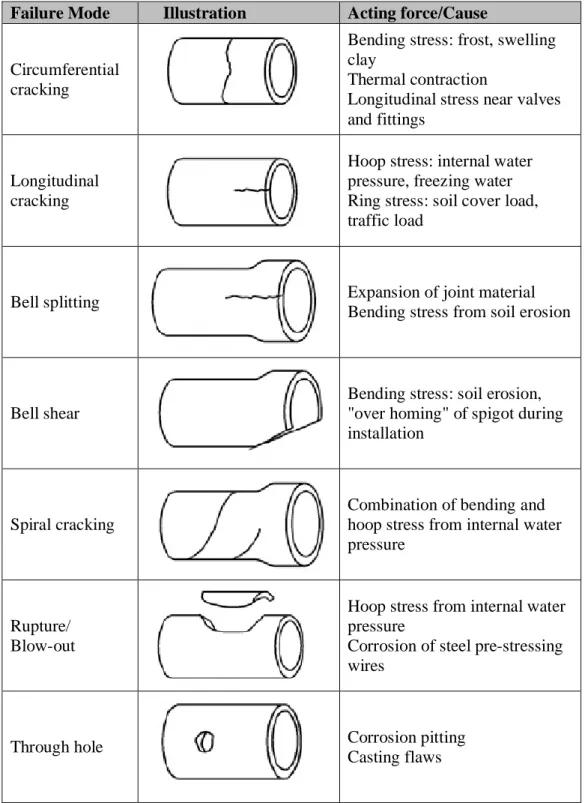
mitigation of collateral damage, the information about the cause of the failure was often not recorded; it was also stated that a degree of specialised engineering background may be required to confidently determine the cause of a failure under a response situation. In other research, Burlingame et al. (1998) also noted that the analyses of pipe failures lacked on-site inspection data. Table 2-1 shows the failure modes with possible causal forces presented by NGSMI (2003).
Table 2-1: Failure modes in water pipes (NGSMI, 2003) Failure Mode Illustration Acting force/Cause
Circumferential cracking
Bending stress: frost, swelling clay
Thermal contraction
Longitudinal stress near valves and fittings
Longitudinal cracking
Hoop stress: internal water pressure, freezing water Ring stress: soil cover load, traffic load
Bell splitting Expansion of joint material
Bending stress from soil erosion
Bell shear
Bending stress: soil erosion, "over homing" of spigot during installation
Spiral cracking
Combination of bending and hoop stress from internal water pressure
Rupture/ Blow-out
Hoop stress from internal water pressure
Corrosion of steel pre-stressing wires
Through hole Corrosion pitting
15
2.4
Factors contributing to pipe failure
The various causes and factors that influence pipe failures have been identified by several authors (e.g. Morris, 1967; Shamir and Howard, 1979; O’Day, 1982; Makondo and Wamukwamba, 2001; Franks and Silinis, 2007). Morris (1967) listed various possible causes of pipe failures and emphasised that determining the cause of a pipe failure is not always possible because a combination of the causes is responsible for the failure. Deb et al. (2002) made recommendations to capture 45 data items for each occurrence of a pipe failure, which indicates just how complex the problem of concluding the cause of a failure can become.
Park (2004) stated the following five major factors affecting water pipe failures: · characteristics of water supply that affect internal corrosion
· internal and external environments · internal and external stresses · type of pipe material
· third party interference
Table 2-2, Table 2-3 and Table 2-4 were adapted from NGSMI (2003) and USEPA (2000) to include surrogate factors, because, as suggested by Wood and Lence (2009), the data typically used and presented in models are surrogates for the actual factors leading to pipe failure.
Table 2-2: Physical factors contributing to failure in water pipes (adapted from NGSMI, 2003; USEPA, 2000; Wood and Lence, 2009)
Factor Explanation Surrogate factor
Physical
Pipe material Pipe made from different materials fail in different ways. Pipe wall
thickness Corrosion will penetrate thinner walled pipe more quickly. Pipe diameter Pipe age Effects of pipe degradation become more apparent over time.
Pipe vintage Pipes made at a particular time and place may be more vulnerable to failure. Pipe age Pipe diameter Small diameter pipes are more susceptible to beam failure.
Type of joints Some joints have experienced premature failure. Pipe material Thrust restraint Inadequate restraint can increase longitudinal stresses. Pipe material, pipe diameter Pipe lining and
coating Lined and coated pipes are less susceptible to corrosion. Pipe material Dissimilar metals Dissimilar metals are susceptible to galvanic corrosion. Pipe material, soil type Pipe installation Poor installation practices can damage pipes, making them vulnerable to failure. Pipe age Pipe manufacture Defects in pipe walls produced by manufacturing errors can make pipes
vulnerable to failure. This problem is most common in older pit cast pipes.
Pipe material, pipe age, pipe lining
16
Table 2-3: Environmental factors contributing to failure in water pipes (adapted from NGSMI, 2003; USEPA, 2000; Wood and Lence, 2009)
Factor Explanation Surrogate factor
Environmental
Pipe bedding Improper bedding may result in premature pipe failure. O&M practices Trench backfill Some backfill materials are corrosive or frost susceptible. O&M practices Soil type
Some soils are corrosive; some soils experience significant volume changes in response to moisture changes, resulting in changes to pipe loading. Presence of hydrocarbons and solvents in soil may result in some pipe deterioration.
Groundwater Some groundwater is aggressive toward certain pipe materials. Pipe material Climate Climate influences, frost penetration and soil moisture. Pipe age, pipe material Pipe location Dynamic traffic loading under roads; road salt migration.
Disturbances
Underground disturbances in the immediate vicinity of an existing pipe can lead to actual damage or changes in the support and loading structure on the pipe.
Stray electrical
currents Stray current cause electrolytic corrosion. Soil type Seismic activity Seismic activity can increase stresses on pipe and cause pressure surges.
Table 2-4: Operational factors contributing to failure in water pipes (adapted from NGSMI, 2003; USEPA, 2000; Wood and Lence, 2009)
Factor Explanation Surrogate factor
Operational
Internal water pressure, transient pressure
Changes in internal water pressure will change stresses acting on the pipe. Leakage Leakage erodes pipe bedding and increases soil moisture in the pipe vicinity.
Water quality Some water is aggressive, promoting corrosion or leaching. Pipe material Flow velocity Rate of internal corrosion is greater in unlined dead-ended mains.
Backflow potential
Cross connections with systems that do not contain potable water can
contaminate water distribution system. O&M practices Poor practices can compromise structural integrity and water quality. Pipe age
A brief discussion of the factors which are commonly reported to have the greatest impact on pipe failure is presented.
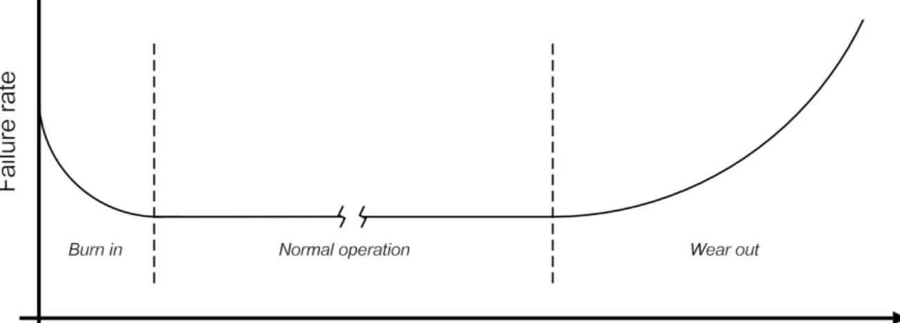
2.4.1 Pipe age
Morris (1967) indicated that pipe age itself is not a cause of pipe failure, as pipe failures occur due to a combination of several factors. The longer a pipe has been in service, the more probable it becomes that the pipe would be affected by various possible causes of pipe failures, such as corrosion, soil movement, temperature differentials and impacts from other infrastructure construction projects. Kleiner et al. (2001) concurred that as the distribution network pipes get older, they are characterised by a decline in hydraulic capacity and an escalated frequency of failures.
17
Rostum (2000) stated that different installation periods demonstrate dissimilar failure characteristics and that these characteristics are more reliant upon the construction practice for each installation period than on the pipe age. As alluded to by Andreou et al. (1987b), some construction periods display a higher failure rate compared to other periods and in many instances the older pipes seem to be more resistant to failure than the younger pipes in the network. Subsequently, Makar et al. (2000) suggested that newer casting methods of cast iron (CI) pipes, which resulted in thinner wall thicknesses, may explain why newer CI pipes had higher failure rates.
Neelakantan et al. (2008) found that, with all other conditions remaining the same, the number of pipe failure events increased with age. Therefore, it is sensible that age should be used as an indicator for forecasting future failure.
The deterioration process can be illustrated by the well-known bathtub curve in Figure 2-3, showing the theoretical failure rate of a pipe in three phases over its service life.
Figure 2-3: Hypothetical failure rate of water pipe over service life 2.4.2 Corrosion
Makar and Kleiner (2000) stated that metallic pipe failure is mainly caused by corrosion. Park (2004) mentioned that the characteristics of the supplied water like pH level, dissolved oxygen, free chlorine residual, temperature, velocity and microbiological activity influence the severity of internal corrosion. The external corrosion is determined by the environment around the pipe (e.g. soil characteristics and ground water) and Kaara (1984) argued that the intensity of external corrosion would vary from pipe to pipe due to the variability in soil conditions. Makar and Kleiner (2000) explained that corrosion can cause failure in non-metallic pipes. For example, pre-stressed wires could corrode and ultimately fail due to internal pipe pressure.
18 2.4.3 Pipe material
Rostum (2000) stated that most of the water distribution pipe infrastructure widely consisted of CI pipes and that long records of failures existed for these pipes, which lead researchers to focus on CI pipe failures. PVC and PE have been introduced for use in water distribution networks, especially for smaller diameter pipes. The characteristics of different pipe materials differ widely and should be considered and analysed separately.
Thornton et al. (2008) stated that globally, municipalities have desisted with the use of asbestos cement (AC) pipes and CI pipes for water distribution network pipes. Many municipalities favour PE or PVC pipes for new installations. A possible disadvantage with so-called plastic pipes is the difficulty reported for detecting peaks at low pressures.
Figure 2-4 was adapted from Mora-Rodriguez et al. (2014) to describe the commercialisation of pipes in water distribution networks. The installation of AC and grey cast CI pipes diminished considerably after the introduction of ductile iron and PVC pipes.
Figure 2-4: Installation periods per material (adapted from Mora-Rodriguez et al., 2014) 2.4.4 Pipe diameter
Small diameter pipes are reported to have the highest frequency of failures, as noted in various studies (e.g. Walski and Pelliccia, 1982; Andreou et al., 1987; Wengström, 1993). Rostum (2000) stated that pipes with diameters ≤ 200 mm usually have exceptionally high number of failures. The higher frequency of failure for smaller diameter pipes could be attributed to thinner pipe walls, reduced pipe strength, less reliable joints and difference in construction standards.
19 2.4.5 Pipe length
Pipe lengths (represented graphically by edges as discussed in paragraph 2.1) differ within a network and also between networks. For long pipes, failure related factors could be non-uniformly distributed along the pipe length (Andreou, 1987b); localised factors that may vary along the length of pipe include differences in soil conditions, traffic loading, tree root growth and inconsistent bedding. Vanrenterghem-Raven (2007) found a strong dependency for some explanatory parameters to the pipe length and argued that the dependency was due to longer pipes having more opportunity for a failure event to occur along their length. Rostum et al. (1997) recommended that pipes should be limited to lengths in the order of 100m to avoid different conditions in one length of the same pipe.
Achim et al. (2007) found that their models’ predictions were significantly worse when length was excluded as an input variable. Pipe length is mainly used to express the number of failures as a rate of occurrence per distance of pipe in the network. In this research, the failure rate is expressed in the number of failures per 100 km per year (
∙ ). 2.4.6 Soil conditions
As stated earlier, soil conditions have an effect on the external corrosion rates and can therefore significantly influence pipe degradation. Morris (1967) discussed soil movement represented by swelling and shrinking soils, which cause weakened pipes to fail more easily. Wood and Lence (2007) also stated that some soils experience volume changes, a factor that puts an additional load on pipes. Wengström (1993) stated that a higher failure rate was reported in clays than in sandy soils. Soil resistivity, which is a measure of the extent to which the soil resists the flow of electricity, also contributes to failures, because stray currents may cause electrolytic corrosion (NGSMI, 2003). Some types of groundwater have also been noted to be aggressive toward certain pipe materials.
2.4.7 Pressure conditions
High static pressure, as well as pressure surges (water hammer), can have a severe impact on pipe failure in a water distribution system. Higher static pressures typically relate to an increased failure rate, as would be expected. Chadwick et al. (2004) noted that pressure surges occur when the flow in the pipe accelerates (or decelerates) due to a change at a controlling boundary and that the intensity of the surge pressure depends on the rate of change at the controlling boundary. Sudden changes in fluid velocity result from common operational causes such as rapid valve closure and pump starts after improper filling practices (Val-Matic, 2009).
20
Pressure surges could be a contributing factor for the phenomenon of failure clustering due to the closing and opening of valves during maintenance and repair activities. Thornton and Lambert (2007) stated that (i) significant reductions in the number of bursts are reported after pressure management, irrespective of pipe materials, and (ii) that pressure is a contributory factor to failure, rather than the prime factor.
2.4.8 Failure history
Walski and Pelliccia (1982) concluded that the failure history of a pipe (number of previous failures) is a significant factor for the prediction of future failures. Goulter et al. (1993) reported on water pipe failure clustering and indicated that the likelihood of future failure for a pipe was increased if another failure occurred in close proximity, and found that about 60% of all subsequent failures occurred within a three month period of a previous failure incident. They suggested that the failure clustering might be caused by damage to the pipes during maintenance operations, such as pressure surge while refilling the pipe, soil movement caused by excavation, substandard backfilling and additional external forces such as the movement of heavy vehicles. Other factors, apart from repair activities, are also responsible for the clustering of failures in a network. Pipes in the same location often have similar failure predictors, such as age, material, external and internal corrosion conditions, installation method and contractor. Misiunas (2005) stated that the failure development history is specific to each pipe and extremely difficult to predict and further noted that the situation becomes even more complicated when failures caused by third party interference are considered.
2.5
Consequence of failure
According to Park et al. (2010) the consequence of physical failure of a component is a measure of the impact on the community and customers. Ispass (2008) stated that the consequence of failure is determined based on a number of institutional factors, including public health, safety, security and level of service.
Sinske and Zietsman (2004) indicated that in addition to disrupting service, water pipe failures also result in significant loss of water, which in equates to a loss in revenue because the water could have been sold to the consumer. They further postulate that in water scarce countries, such as South Africa, water losses can negatively impact the living standard of people. Flooding as a result of pipe bursts can furthermore cause extensive damage to nearby lower-lying properties. Neelakantan et al. (2008) stated that interruption of supply to water-intensive industries, traffic disruptions, disease outbreaks and delays in firefighting ability are also possible consequences of water pipe failures.
21
The impact associated with a pipe failure can be divided into three main categories, namely direct costs, indirect costs and social costs. These three categories are discussed briefly below.
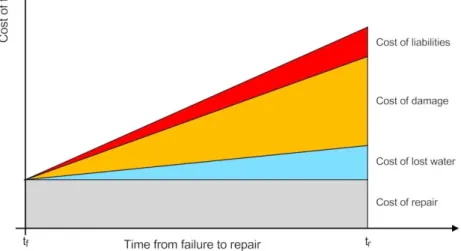
2.5.1 Direct costs
Direct costs refer to expenditure directly related to the current occurrence of the pipe failure. These are more easily quantified and calculated when compared to indirect costs, and even more so when compared to social costs. The direct costs are a summation of the following costs:
· Cost of repair. · Cost of lost water.
· Cost of damage to adjacent infrastructure (flooding, road collapse, etc.). · Cost of liabilities (injury, accidents, structural damage, etc.).
The direct costs depend on the parameters of a pipe such as diameter, material and location, as well as the severity of the failure, time to isolation of the failure and the production and conveyance cost of water. Figure 2-5 depicts an example of the increase in direct costs incurred from the time of failure (tf) to the time of repair (tr). The costs are not necessarily linear functions
of time, but a linear function was used for illustration.
Figure 2-5: Direct costs due to a failure over time (adapted from Misiunas, 2005) 2.5.2 Indirect costs
Indirect costs refer to the inability of the system to achieve its purpose and possible expenditure that was not accounted for, which increases overall cost of failure as shown in Figure 2-6. A linear function of time is used for illustration as for the direct costs.
22 The indirect costs are described as follows:
· Cost of supply interruption – loss of business due to non-supply of water.
· Cost of possible increase in deterioration rate of surrounding infrastructure and subsequent devaluation.
· Cost of diminished ability for fire-fighting.
Figure 2-6: Direct and indirect cost of failure (adapted from Misiunas, 2005)
2.5.3 Social costs
Social costs are heavily influenced by the location of the failure and the time to isolation of the affected part of the network by closing the appropriate network isolation valves. The social costs are less tangible in nature and described as:
· Cost of water quality degradation – contaminant intrusion from depressuring. · Cost of customer inconvenience – decrease in public trust.
· Cost of disruption to the traffic and businesses. · Cost of insufficient supply to special facilities.
23
2.6
Failure prediction models
USEPA (2000) presented different approaches to failure prediction classified in the following three major modelling groups: (i) probabilistic or statistical models, (ii) deterministic methods and (iii) heuristic methods. Clair and Sinha (2012) presented a comprehensive review on different water pipe condition, deterioration and failure rate prediction models, and proposed that each of the models be grouped into one of the following six categories: (i) deterministic, (ii) statistical, (iii) probabilistic and advanced mathematical models which consist of (iv) artificial neural networks (ANN), (v) fuzzy logic and (vi) heuristic models. Tabesh et al. (2009) combined the ANN and fuzzy logic models into so-called data-driven modelling techniques.
Previously published failure prediction models from literature were reviewed and summarised as part of this research. Physical or mechanistic models and models that focus on single material types were excluded. The models are presented in chronological order in the following tables:
· Table 2-5: Time-relationship models, · Table 2-6: Failure-clustering models,
· Table 2-7: Probabilistic and statistical models, · Table 2-8: Bayesian models and