DIFFERENTIAL
EXPRESSION
AND
FEATURE
SELECTION
IN
THE
ANALYSIS
OF
MULTIPLE
OMICS
STUDIES
by
Tianzhou
Ma
MS
in
Biostatistics,
Yale
University,
2013
BS
in
Genetics
and
Biotechnology
(specialist),
University
of
Toronto,
Canada,
2010
Submitted
to
the
Graduate
Faculty
of
the
Department
of
Biostatistics
Graduate
school
of
Public
health
in
partial
fulfillment
of
the
requirements
for
the
degree
of
Doctor
of
Philosophy
University
of
Pittsburgh
UNIVERSITY OFPITTSBURGH
GRADUATESCHOOL OF PUBLICHEALTH
This dissertation was presented
by
TianzhouMa
It wasdefended on
March2nd, 2018
and approvedby
George C. Tseng,ScD, Professor, Departmentof Biostatistics, Graduate Schoolof Public Health, University of Pittsburgh
Zhao Ren, PhD,Assistant Professor, Departmentof Statistics, Dietrich Schoolof Arts and Sciences, University of Pittsburgh
Faming Liang, PhD,Professor, Department of Statistics, PurdueUniversity, West Lafayette, Indiana
Ying Ding,PhD, Assistant Professor, Department of Biostatistics,Graduate School of Public Health, University of Pittsburgh
Robert Krafty, PhD, Associate Professor, Department of Biostatistics,Graduate School of Public Health, Universityof Pittsburgh
DissertationAdvisors: George C. Tseng, ScD, Professor,Department of Biostatistics, Graduate School of Public Health,University of Pittsburgh
Zhao Ren, PhD, Assistant Professor, Department of Statistics, Dietrich School of Arts and Sciences, University of Pittsburgh
Copyright cby Tianzhou Ma 2018
DIFFERENTIAL EXPRESSION AND FEATURE SELECTION IN THE ANALYSIS OF MULTIPLE OMICS STUDIES
Tianzhou Ma, PhD
University of Pittsburgh, 2018
ABSTRACT
With the rapid advances of high-throughput technologies in the past decades, various kinds of omics data have been generated from many labs and accumulated in the public domain. These studies have been designed for different biological purposes, including the identification of differentially expressed genes, the selection of predictive biomarkers, etc. Effective meta-analysis of omics data from multiple studies can improve statistical power, accuracy and reproducibility of single study. This dissertation covered a few methods for differential expression (Chapter 2 and 3) and feature selection (Chapter 4) in the analysis of multiple omics studies.
In Chapter 2, we proposed a full Bayesian hierarchical model for RNA-seq meta-analysis by modeling count data, integrating information across genes and across studies, and mod-eling differential signals across studies via latent variables. A Dirichlet process mixture prior was further applied on the latent variables to provide categorization of detected biomarkers according to their differential expression patterns across studies. We used both simulations and a real application on multiple brain region HIV-1 transgenic rats to demonstrate im-proved sensitivity, accuracy and biological findings of our method. In Chapter 3, we extended the previous Bayesian model to jointly integrate transcriptomic data from the two platforms: microarray and RNA-seq.
In Chapter 4, we considered a general framework for variable screening with multiple omics studies and further proposed a novel two-step screening procedure for high-dimensional
regression analysis in this framework. Compared to the one-step procedure and rank-based sure independence screening procedure, our procedure greatly reduced false negative errors while keeping a low false positive rate. Theoretically, we showed that our procedure possesses the sure screening property with weaker assumptions on signal strengths and allows the number of features to grow at an exponential rate of the sample size.
Public health significance:
The proposed methods are useful in detecting important biomarkers that are either differen-tially expressed or predictive of clinical outcomes. This is essential for searching for potential drug targets and understanding the disease mechanism. Such findings in basic science can be translated into preventive medicine or potential treatment for disease to promote human health and improve the global healthcare system.
TABLE OF CONTENTS
PREFACE . . . xiii
1.0 INTRODUCTION . . . 1
1.1 Overview of High-throughput omics data and technologies . . . 1
1.1.1 Genomic data . . . 1
1.1.2 Transcriptomic data . . . 3
1.1.3 Other omics data . . . 4
1.1.4 High-throughput technologies in omics research . . . 5
1.1.4.1 Microarray . . . 5
1.1.4.2 Next generation sequencing . . . 6
1.1.5 Public resource of omics data . . . 7
1.2 Objectives of omics studies and relevant analysis. . . 9
1.2.1 Differential expression analysis . . . 9
1.2.2 Regression analysis with feature selection . . . 11
1.2.3 Clustering and network analysis . . . 13
1.3 Data integration and meta-analysis . . . 14
1.3.1 Horizontal meta-analysis. . . 14
1.3.2 Vertical integrative analysis . . . 15
1.4 Fundamentals of Bayesian data analysis and its application in omics studies 16 1.5 Overview of the dissertation . . . 18
2.0 RNA-SEQ META-ANALYSIS USING BAYESIAN HIERARCHICAL MODEL . . . 20
2.2 Bayesian Hierarchical Model . . . 23
2.2.1 Notation and Assumptions . . . 23
2.2.2 Generative model within each study . . . 24
2.2.3 Information integration of effect size across studies among DE genes 25 2.2.4 Model-based clustering to categorize DE genes . . . 27
2.2.5 Simulating posterior distribution via MCMC . . . 28
2.3 Bayesian inference and Clustering . . . 29
2.3.1 Bayesian inference and control of false discovery rate . . . 29
2.3.2 Summarization of clustering posterior to categorize DE genes . . . . 30
2.3.3 Methods for comparison . . . 31
2.4 Simulation . . . 32
2.4.0.1 Simulation I, II . . . 34
2.4.0.2 Simulation III . . . 34
2.5 Real Data Analysis . . . 37
2.5.1 Differential expression analysis . . . 37
2.5.2 Pathway enrichment analysis on detected DE genes . . . 38
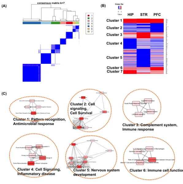
2.5.3 Categorization of DE genes by study heterogeneity . . . 41
2.6 Discussion and Conclusion . . . 43
3.0 INTEGRATING MICROARRAY AND RNA-SEQ TRANSCRIPTOMIC DATA USING BAYESIAN HIERARCHICAL MODEL . . . 46
3.1 Introduction . . . 46
3.2 Methods . . . 50
3.2.1 Notation . . . 50
3.2.2 Bayesian Hierarchical Model . . . 50
3.2.3 Normalization Algorithm . . . 53
3.2.4 Evidence for necessity of normalization . . . 54
3.2.5 Inference for Differential Expression . . . 55
3.2.6 Methods for comparison . . . 57
3.3.1 Simulation . . . 57
3.3.2 Application . . . 58
3.4 Discussion and Conclusion . . . 67
4.0 VARIABLE SCREENING WITH MULTIPLE STUDIES . . . 71
4.1 Introduction . . . 71
4.2 Model and Notation . . . 73
4.3 Screening procedure with multiple studies . . . 75
4.3.1 Sure independence screening . . . 75
4.3.2 Two-step screening procedure with multiple studies . . . 76
4.4 Theoretical properties . . . 80
4.4.1 Assumptions and conditions . . . 80
4.4.2 Consistency of the two-step screening procedure . . . 82
4.4.3 Partial faithfulness and Sure screening property . . . 82
4.5 Algorithms for variable selection with multiple studies. . . 84
4.5.1 Multi-PC algorithm . . . 84
4.5.2 Two-stage feature selection . . . 86
4.6 Numerical evidence . . . 86
4.7 Real data application . . . 88
4.8 Discussion . . . 91
5.0 DISCUSSION AND FUTURE WORKS . . . 93
5.1 Discussion . . . 93
5.2 Extension of the screening procedure to non-linear case . . . 94
APPENDIX A. APPENDIX FOR “BAYESMETASEQ”. . . 95
A.1 Parameter estimation by Gibbs Sampling and the Metropolis-Hastings algo-rithm . . . 95
A.2 Supplemental figures and tables . . . 99
APPENDIX B. APPENDIX FOR “CBM” . . . 107
B.1 Sample the posterior distribution by MCMC . . . 107
B.2 Simulation results: ROC and PR curves . . . 110
APPENDIX C. APPENDIX FOR “TSA-SIS” . . . 112
C.1 Proofs . . . 112
LIST OF TABLES
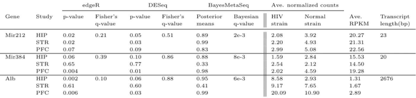
1 Comparison of three approaches in real rat data . . . 39
2 Three example genes that show better detection power of BayesMetaSeq to detect low expressed or short length genes. . . 39
3 Selected GO pathways enriched only with BayesMetaSeq from Figure 4(B). . 41
4 Number of DE genes detected by five approaches at varying cutoff . . . 63
5 ILC stage: Three example genes that show the necessity of applying normal-ization . . . 63
6 ILC stage: Selected top pathways enriched with BayesNorm . . . 66
7 ILC PR: Three example genes that show the necessity of applying normalization 67
8 ILC PR: Selected top pathways enriched with BayesNorm . . . 68
9 Toy example to demonstrate the strength of two-step screening procedure. . . 79
10 Sensitivity analysis on the choice of α1 and α2 in simulation . . . 88
11 The six genes selected by our TSA-SIS procedure. . . 90
12 Comparison of parameters estimates by BayesMetaSeq with their true values from Simulation IA, K=2 . . . 100
13 Sensitivity analysis on hyperparameter µη . . . 100
14 Normalized counts(rounded) for the three genes shown inTable 2. . . 103
15 List of significant IPA pathways (p-value< 0.05) from Cluster 1-4 in Figure 6. 105
16 List of significant IPA pathways (p-value< 0.05) from Cluster 5-7 in Figure 6. 106
LIST OF FIGURES
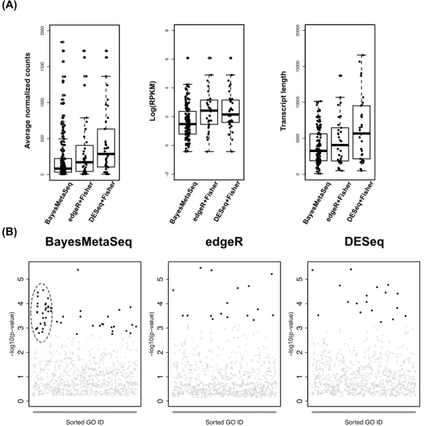
1 Measuring gene expression: DNA microarray vs. RNA-seq . . . 8
2 “BayesMetaSeq”: Graphical representation of the Bayesian hierarchical model 24 3 ROC Curve (left) and Power (right) comparison of the three methods . . . . 35
4 Clustering results from Simulation III . . . 36
5 Comparison of three methods in real rat RNA-seq data . . . 40
6 Real rat data clustering results . . . 42
7 “CBM”: Graphical representation of the Bayesian hierarchical model . . . 51
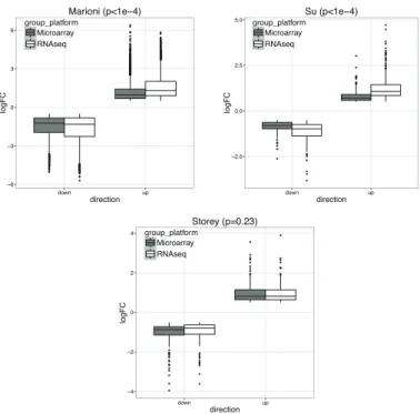
8 Boxplot of logFC from either microarray or RNA-seq in three public studies . 56 9 Power comparison of different methods in simulation . . . 59
10 Cross-platform logFC comparison . . . 61
11 Comparison of significance of RNA-seq vs. microarray in BayesNorm detected DE genes . . . 64
12 GO enrichment analysis results using the top 500 genes from the two methods 66 13 Simulation results 1-4 . . . 89
14 Traceplots of selected parameters from Simulation IA. . . 101
15 Venn Diagram of number of overlapping DE genes (FDR < 0.1) among the three methods applied in real data . . . 102
16 Distributionof normalizedcounts for the three genes shown inTable 2 . . . . 104
PREFACE
This dissertation covers the major methodology work during my five years’ PhD studies and builds upon a foundation of excellent mentorship, generous peer support and endless love from the family. First of all, I would like to express the most genuine gratitude to Dr. George Tseng, my main advisor who really brings me to the world of “omics” and guides me how to do good research. He has been so knowledgable, patient and helpful, and serves as a role model scientist and statistician for fresh PhDs and young researchers like me. As a renowned faculty and experienced mentor, he still keeps a low profile and always stays humble, and most of time when we talk and discuss the research, he is more like a friend rather than an advisor. Having the chance to work with him and in his research group is my great honor and I will benefit from it for my entire academic career.
Next, I want to thank my co-advisor Dr. Zhao Ren for his advising on the sure screening paper. I took quite some theoretical courses he offered and became interested in theoretical statistics even if I came from a biological background in undergraduate. I really learnt a lot from him through classes and research and admired his persistent efforts in popularizing the education in statistical theory to students in biostatistics like me. I want to thank Dr. Faming Liang, for providing selfish guidance to me in the first two Bayesian papers, when the Bayesian statistics was still very new to me.
I also want to thank all my other committee members Dr. Ying Ding and Dr. Robert Krafty for providing me a great amount of help and advices on my research, presenting skills and career development.
I want to thank all my former and current lab mates for their support and help in both research and daily life. Without them, I would not have been productive during my PhD studies. Without them, I would have been lonely and may have lost my passion in research.
I would also like to thank my collaborators, Dr. Etienne Sibille from the Centre for Addiction and Mental Health (CAMH), University of Toronto, Drs. Steffi Oesterreich, Anda Vlad and Faina Linkov from Magee-Womens Research Institute (MWRI), who have helped me acquire a lot of collaborative publications and motivated me to think about new method-ologies to solve statistical issues in biomedical applications of their fields.
I want to show my deepest gratitude to my parents, Xiaoyun and Aiguang, for their support both spiritually and materially. I am so lucky to have such open-minded parents like you two, you have always been hard-working, sincere and kind to others, and have set an example for me. I also want to thank my other family members, my aunt Yue and my cousin Jing for bringing the joy to life, my uncle Zhan for his positive influence on my attitude towards life and academics, my parents in law Cuifeng and Xiaomin for giving me and Zhongying the best care.
Lastly, I would like to express my greatest gratitude to my lifetime lover, my wife Zhongy-ing. The path to an academic career is a long journey with all kinds of hardship, I am lucky to have you accompany in this journey. Thank you for your willingness to sacrifice the fa-vorable conditions in China and stay and study in the States with me in the past six years and probably in the future. Thank you for all your contribution to the family and your understanding when I spent more time in research than being with you. Thank you and always love you and our little one.
1.0 INTRODUCTION
1.1 OVERVIEW OF HIGH-THROUGHPUT OMICS DATA AND
TECHNOLOGIES
The rapid advances and prevalence of various high-throughput experimental technologies have generated abundant omics data in the public repositories in recent years and effective analytical approaches are crucial to fully understand the biological knowledge inside these data. Ending with the same suffix, these “-omics” data are used to study an organism’s ge-netic material (“Genomics”), RNA transcripts (“Transcriptomics”), proteins (“Proteomics”), epigenetic modification (“Epigenomics”), etc., all of which play essential roles in the flow of biological information in the central dogma paradigm (DN A ↔ RN A → P rotein). This section will briefly introduce the various types of omics data, the two major plat-forms/technologies that generate these data and the public repository and databases of omics datasets.
1.1.1 Genomic data
Genomics is the study of the complete set of genetic material within an organism usually consisting of DNA (RNA for some viruses). Unlike genetics which studies individual genes, it usually applies high-throughput technologies such as DNA sequencing to assemble and analyze the function and structure of entire genomes including both coding and noncoding regions.
The human genome contains approximately 3.2×10⁹ base pairs distributed among 22
for only 1.5% of the whole genome (Lesk, 2017). The average proportion of nucleotide differences among different human individuals has been consistently estimated to lie between 1 in 1,000 and 1 in 1,500 (Jorde and Wooding, 2004). Considering this nucleotide diversity, personal genomics is the branch of genomics that focused on determining the genetic make-up (a.k.a. genotype) of an individual and comparing to another individual’s sequence or a reference sequence.
Genetic variation among individuals can be attributed to independent assortment, cross-over and recombination during meiosis as well as various mutational events. Mutation is a permanent alteration of nucleotide sequence in the genome and the resulting change of DNA is not repairable and the errors will proceed to DNA replication and RNA transcription. It is associated with abnormal biological processes like cancer since changes in DNA can cause errors in protein sequence, creating partially or completely non-functional proteins. There are two types of major mutations: somatic mutation and germline mutation. Somatic mutation takes place in somatic cells and is usually caused by environmental factors. It is neither inherited from parents nor passed to offsprings. Germline mutation occurs in reproductive cells such as sperm or ova and is inheritable. This type of mutation can be transmitted to offspring.
Among the various types of genetic variation, single nucleotide polymorphism (SNP) is the most common one and represents difference in a single nucleotide between members that occurs in at least 1% of the population. Single-nucleotide variant (SNV) is a variation in a single nucleotide without any limitations of frequency and may arise in somatic cells. Genome-wide association study (GWAS) is known as a popular design to assess thousands to millions of common SNPs associated with a disease or a trait. Thousands of disease-susceptible variants have been discovered through the GWAS of hundreds or thousands of individuals (Hindorff et al.,2009;McCarthy et al., 2008). Recently, rare-variant association analysis has aroused more interest in the field which focuses on rare variants that might explain disease risk or trait variability in addition to common variants found in GWAS (Lee et al., 2014).
Other types of genetic variation include insertion/deletion (“indel”) polymorphism in which a specific nucleotide sequence is present or absent; copy number variation (CNV),
a structure variation of DNA segment due to deletion or duplication of large regions of DNA on some chromosome. CNV has been found to be related with disease phenotype and also account for regulation of genes expression and other genomic process (McCarroll and Altshuler, 2007).
1.1.2 Transcriptomic data
Transcriptomics studies the sum of all RNA molecules (a.k.a. transcripts) in an organism or in a cell, including messenger RNA (mRNA), ribosomal RNA (rRNA), transfer RNA (tRNA) and other non-coding RNA such as microRNA (miRNA), etc. Unlike the genome which is almost fixed for a given cell line, the transcriptome only reflect genes that are expressed at given time and can vary with different external conditions. Microarray and RNA sequencing (RNA-seq) are the two major platforms to quantify the transcriptome and will be introduced in the next section.
mRNA is the major family of RNA molecules that convey genetic information from DNA (known as “transcription”) and produce proteins (known as “translation”). In eukaryotes, mRNA is first transcribed into precursor mRNA (pre-mRNA) and has to undertake a few processing steps including 5’ cap addition, polyadenylation and splicing before it matures to generate proteins. Splicing is the editing process that removes introns (intervening se-quence) from RNA and joins exons (the actual coding part of a gene) together. Since a gene contains multiple exons and mature mRNAs from the same gene can include different exons, alternative splicing can take place and produces multiple protein isoforms in the translation stage. Distinct from the stable DNA molecules, mRNA molecules have a short half life and will ultimately end in degradation.
Other RNA molecules, though not necessarily translated into protein products, play important roles in regulating and catalyzing the transcription, translation and other biolog-ical processes inside the cell. For example, rRNAs are basic components of the ribosome and catalyze the transcription; tRNAs transfers specific amino acids to a growing polypep-tide to synthesize protein during translation; miRNAs function in RNA silencing and post-transcriptional regulation of gene expression.
Genetics have effects on the transcriptome. Expression quantitative trait loci (eQTLs) are genomic loci that contribute to variation in mRNA expression. Using RNA-seq samples from the 1000 Genome project, recent studies uncovered extremely widespread regulatory variation, with 3773 genes having a classical eQTL for gene expression levels (Lappalainen et al., 2013). Based on the distance to their gene-of-origin, eQTLs can be further divided into two types: cis-eQTLs (locally) and trans-eQTLs (at a distance).
1.1.3 Other omics data
There are other important omics data that are not the focus of this thesis, for example the epigenomics and the proteomics.
Epigenome is the complete set of epigenetic modifications, including DNA methylation, histone modification and chromatin structure change. It plays an indispensable role in gene expression and regulation and partially determines one’s phenotype in addition to genotype and environment (Lesk, 2017). DNA methylation is the process methyl groups are added to nucleotides in DNA and is associated with a number of key processes, e.g. genomic imprinting, X-chromosome inactivation, silencing of repetitive DNA, etc. (Sch¨ubeler,2015). Methylation takes place at the cytosine nucleotide in eukaryotes and when it is followed by a guanine nucleotide it forms a CpG site. Approximately 60% of CpG sites are methylated in somatic cells in vertebrates and those DNA regions with high frequency of CpG sites are also called CpG islands (Bird,2002). To quantify the methylation level, scientists define the beta value for a CpG site as the percentage of methylated events out of all events which ranges between 0 and 1. The alteration of DNA methylation pattern has been outstanding in cancer, where the loss of expression of genes is about 10 times more frequently by hypermethylation of CpG islands in the promoter region than by mutations (Vogelstein et al., 2013).
Proteomics studies the entire set of protein products in an organism. Proteins are made up of long chains of amino acids with 3D configuration and perform vast array of functions inside the body. Like the transcriptome, proteome also varies with time and condition in given cell or system. To detect and quantify proteins, researchers either apply antibody-based methods (immunoassays) or mass spectrometry-antibody-based techniques. In addition to the
expression profiling of proteins, computational biologists also use technologies like X-ray crystallography and NMR spectroscopy to perform structural analysis of proteins looking for e.g. potential drug binding sites.
There are multiple levels of molecular variation from different omics data that contribute to disease risk in a nonlinear, interactive and complex way and there also exist cross-talk among different types of omics data (Ritchie et al., 2015). For example, like eQTLs, re-searchers also characterized DNA methylation quantitative trait loci (mQTLs) and showed their important functions especially in the brain (Hannon et al., 2016). Other examples include ChIP-sequencing (ChIP-seq) which combines chromatin immunoprecipitation and DNA sequencing and is used to analyze protein (e.g. transcription factor) interaction with DNA.
1.1.4 High-throughput technologies in omics research
1.1.4.1 Microarray Before the advent of microarray techniques, biologists use northern plot or quantitative Polymerase Chain Reaction (qPCR) to study and quantify gene expres-sion. These techniques are time consuming and expensive, since they perform gene-by-gene analysis and can only detect up to dozens of genes. As one of the earliest high-throughput technologies, the invention of DNA microarray in the early 1990s marks the start of the omics era and makes it possible to measure the expression levels of thousands of genes up to the whole genome or to genotype multiple regions of a genome simultaneously. In its application to gene expression profiling, tens of thousands of transcript-specific probes are immobilized on a solid support, such as a microscope glass slide or silicon chips, to make up the “microarray.” RNA samples are reversely transcribed to cDNA, fluorescently labeled, amplified and hybridized to the microarray. The array is then washed and the expression level is quantified by measuring fluorescence intensity at each spot (Figure 1 left). In ad-dition to gene expression profiling, the microarray technique can also be applied to detect SNPs, CNVs, DNA methylation, and protein-DNA binding.
There are a few limitations with DNA microarrays. First, microarray has detection limit at the lower end thus the intensities of low-expressed genes are un-distinguishable from
background noise; Secondly, microarray only provides an indirect measure of relative con-centration, at high concentrations it will become saturated and at low concentrations the equilibrium will favor no binding; Finally, DNA microarray can only detect known sequences it was designed to detect (Bumgarner, 2013;Mortazavi et al.,2008). Due to these disadvan-tages, microarray is now gradually being replaced by the newer RNA-seq technique for gene expression profiling.
1.1.4.2 Next generation sequencing In the past decade, there has been a fundamen-tal shift from the more traditional Sanger sequencing to the next-generation sequencing (NGS) for genomic analysis. With run time as short as a few hours to sequence the whole genome of a sample, the arrival of NGS technologies has changed the way we think about scientific approaches in basic, applied and clinical research (Metzker, 2010). NGS is also called ultra-high-throughput sequencing which can process millions of sequence reads simul-taneously and have been widely applied to genome sequencing (whole genome sequencing and whole exome sequencing), transcriptome profiling (RNA-seq), DNA methylation (bisul-fite sequencing), DNA-protein interaction (ChIP-sequencing), etc. In a typical RNA seq workflow, the cDNA samples are chopped into DNA fragments (called “reads”) with specific adapter oligos bound to both ends and the DNA fragments are then sequenced. The reads generated by sequencers can vary by read lengths depending on user preference, technolo-gies or platforms (e.g. Illumina, SOLiD, Roche). The sequenced reads are reassembled and aligned to a reference genome to quantify the expression levels of genes or transcripts by counting the number of mapped short reads (Figure 1right).
Comparing to the DNA microarray, RNA-seq has quite a few advantages. First, RNA-seq has higher sensitivity and accuracy in quantifying the low-expressed genes; Secondly, RNA-seq can be used to detect novel transcripts or isoforms which is impossible in microarray with only known probes. Last but not the least, it can also be used to examine transcriptome fine structure such as allele-specific expression and splice junctions (Wang et al., 2009).
As shown in Figure 1, DNA microarray will generate a matrix of continuous intensity values while RNA-seq will generate a matrix of count data after a series of preprocessing steps for each platform. If we perform some normalization by both library size (i.e. total counts
in a sample) and gene length, we can also generate continuous values such as RPKM (Reads Per Kilobase Million) or FPKM (Fragments Per Kilobase Million) or TPM (Transcripts Per Kilobase Million) from RNA-seq. However, such normalization introduces a length bias into the variance and is less powerful than the count data (Oshlack and Wakefield, 2009). The first paper of my thesis proposed a new method to integrate multiple RNA-seq count data and the second paper extended the method to integrate continuous data from microarray and count data from RNA-seq.
1.1.5 Public resource of omics data
With the rapid advances of high-throughput technologies and their reduction in cost in the past decades, generation of various kinds of omic data becomes affordable and prevalent in many labs. For example, large amount of transcriptomic data have been accumulated from microarray or RNA-seq experiments for different biological aims and have been stored in large data repositories such as Gene Expression Omnibus (GEO), ArrayExpress and Sequence Read Archive (SRA). Hundreds of GWAS studies have been conducted since 2000s and many datasets are stored in database of Genotypes and Phenotypes (dbGaP). In addition to these public available databases, many worldwide and nationwide consortium projects were launched in the last 10 to 15 years for different aims and generated omics data with large sample size and high quality to serve the whole scientific community. For instance, The Cancer Genome Atlas (TCGA), a “community resource project” initiated by National Cancer Institute (NCI), has profiled and analyzed a total of 33 cancer types including 10 rare cancers and generated rich amount of data at the DNA (mutation, copy number variation, etc.), RNA (gene expression, miRNA expression, etc.), protein (protein expression) and epigenetic (DNA methylation) levels. The Encyclopedia of DNA Elements (ENCODE) is a public research project aiming to identify and annotate all functional elements in the human genome including both coding and non-coding parts. The MODel organism ENCyclopedia Of DNA Elements (modENCODE) project further extends the original ENCODE project to identify the functional elements in selected model organism genomes. For omics data from in vitro cell
cultures or immortal cell lines, the Cancer Cell Line Encyclopedia (CCLE) project conducted detailed genetic characterization (copy number variation, mRNA expression, mutation and more) for more than 1,000 cancer cell lines (Barretina et al., 2012).
The affluent omics datasets in the public domain provide opportunities and have mo-tivated us to combine data from multiple cohorts (from different platforms) for different biological purposes such as differential expression analysis (paper 1 & 2) and prediction analysis with feature selection (paper 3)
1.2 OBJECTIVES OF OMICS STUDIES AND RELEVANT ANALYSIS
The various omics studies mentioned above are designed for different biological purposes. For transcriptomic studies, the most common purpose is to identify genes that are differentially expressed among predefined classes, e.g. between the diseased patients and normal controls. In addition, researchers are also interested in identifying important biomarkers (e.g. genes, SNPs, etc.) that can predict clinical outcomes or classify new patients. Some experiments are designed to identify novel subtypes based on the omics data, and other experiments aim at exploring the relationship among the genes or proteins via biological networks. In this section, I will briefly introduce these biological objectives and the types of statistical analysis involved.
1.2.1 Differential expression analysis
An important task in genomic data analysis is to identify candidate markers associated with the disease status, disease progression or environmental perturbation. In a two class com-parison scenario, genomic comparative studies applied differential expression (DE) analysis methods on microarray or RNA-seq data to select genes that are differentially expressed between case and control.
The gene expression data from microarray is continuous and usually normally distributed. In the simplest scenario, we can fit the following linear model for each gene to test whether it is differentially expressed: ygi =αg+βgXi+ P X p=1 γpgZpi,
where ygi is the expression value for the gth gene and ith sample, Xi the indicator of the condition (e.g. 1 for case and 0 for control), αg is the gene-specific intercept andZpi indicate the known confounding covariates you wish to adjust. The purpose is to test whether βg is zero or not. Simple linear model via e.g. traditional t-test will underestimate variance by chance when the sample size n is small but the number of genes G is large, to overcome , Smyth (2004) proposed a specific linear model for microarray data (called “LIMMA”) using empirical Bayes approach and suggested a moderated t-statistics by shrinking the estimated sample variances towards a pooled estimate for more stable inference (Smyth, 2005). SAM (short for “Significance Analysis of Microarray”) is another popular tool for differential analysis in microarray that uses nonparametric statistics (Tusher et al., 2001).
For count data obtained from RNA-seq, the linear model has to be extended to a gener-alized linear model (GLM) setting:
g(E(ygi)) =Ti+αg+βgXi+ P X p=1
γpgZpi,
where ygi is the expression value for the gth gene and ith sample, g(.) is the link function (usually use “log”), Ti is the offset of ith sample adjusting for the sequencing depth of each sample and αg is the gene-specific intercept. Negative binomial distribution is a more popular choice than Poisson to fit y nowadays since over-dispersion is commonly seen in RNA-seq data. edgeR and DESeq are the two most widely used tools for the differential expression analysis in RNA-seq, both of which are under the GLM framework with more careful estimation of the dispersion parameter (McCarthy et al., 2012; Anders and Huber,
2010).
For DE analysis of high-dimensional genomic data, multiple comparison is one big issue always needs to be addressed. There are two general categories of methods for multiple
comparison correction in the literature. The first category aims to control for the family-wise error rate (FWER) (Hochberg and Tamhane, 2009), corresponding to the probability of making at least one false discovery. Common methods falling in this category includes the Bonferroni procedure which is a popular choice in GWAS. However, such methods are usually too stringent for DE analysis in transcriptomic studies. The second less stringent category is designed to control the false discovery rate (FDR) (Benjamini and Hochberg,
1995), defined as the expected proportion of false positives among all positive “discoveries” (i.e. the type I error). Methods under this alternative category such as Benjamini-Hochberg procedure or Bayesian FDR are more popular choices in genomic studies.
The identification of important biomarkers are useful to narrow down target for further investigation, however, they may still contain little unifying biological theme for most re-searchers. Thus, the pathway analysis (a.k.a. gene set enrichment test) usually following the DE analysis is applied for functional annotation of the identified gene list, based on one or multiple known pathway database. Commonly used pathway databases include Gene Ontology (GO), Kyoto Encyclopedia of Genes and Genomes (KEGG), Reactome, etc.
The first and second papers in this dissertation proposed new methods for differential expression analysis when there are multiple transcriptomic datasets from multiple platforms.
1.2.2 Regression analysis with feature selection
In statistics, regression can be used to explore the relationship between independent variables and a dependent variable. When there are many independent variables present (i.e. multiple regression), we wish to identify those that are most predictive of the dependent variable. In omics studies, this might include the identification of genes or SNPs that can predict the disease status, survival or some specific quantitative measures, etc. When the outcome is binary or categorical, it becomes a classification problem in machine learning.
Consider a linear regression setting with n samples and p features (e.g. genes):
yi =β0 +
p X
j=1
where yi is the outcome for the ith sample, Xij is the (expression) value for the ith sample andjth feature andi is the error term. This regression model is very different from the one in the DE analysis, where y corresponds to the feature.
Very frequently in omics studies, we are facing the high-dimension data with “small n, large p” (p >> n). In that case, the matrix X is singular and most parameters are not identifiable. Conventional methods such as principal component analysis (PCA) or singular value decomposition (SVD) can be applied onXto reduce dimension, however, such implementation will lose the individual feature identity and interpretability. Alternatively, regularization approaches can be applied to solve such ill-posed regression problem. Over the past two decades, many regularization methods have been developed and can be summarized in the form penalized likelihood by solving the following objective function:
ˆ
β =argmin
β (||y−Xβ||
2+λ||β||
q),
where λ is penalty parameter. When q = 0 (L0 norm), it becomes the traditional model
selection by AIC/BIC; whenq= 1(L1norm), this is the least absolute shrinkage and selection
operator (LASSO) (Tibshirani, 1996; Zou, 2006); when q = 2 (L2 norm) this is the group
version of the LASSO (Yuan and Lin, 2006); when the square of L2 norm is used, this is
the ridge regression; when both L1 norm and L2 norm are used, this is the elastic net (Zou and Hastie, 2005). In particular, LASSO method and its extensions (i.e. group LASSO, elastic net, adaptive LASSO, etc.) induce sparsity in the regression model and achieve the goal of feature selection. In the Bayesian school, the feature selection is achieved by putting sparsity-induced priors like Spike-and-slab prior (George and McCulloch, 1993; Ishwaran and Rao, 2005) or shrinkage priors like Laplace prior (a.k.a. Bayesian LASSO) (Park and Casella,2008).
However, when p is very large, the computational cost can be a hurdle for most regu-larization methods and some theoretical assumptions may no longer hold. Sure screening methods such as sure independence screening (SIS) have been proposed as a natural way to select relevant variables based on their marginal correlation (Fan and Lv, 2008). The gen-eral idea is to first reduce a high dimensional model to a relatively lower dimensional model which still contains the true model almost surely via sure screening and then performs model
selection using one of the aforementioned regularization approaches. With improvement in both speed and performance, sure screening methods have gained more popularity in various statistical fields these years.
The third paper of this dissertation proposed a new screening method for the scenario when datasets from multiple homogeneous studies are present.
1.2.3 Clustering and network analysis
In addition to those mentioned above, there are many omics studies designed for other biological purposes and applied different analysis approaches.
When the class labels are unknown, researchers will apply clustering analysis looking for novel subtypes based on e.g. gene expression profiles of the samples, which could serve as a guide to precision medicine. There are two major classes of clustering methods: distance-based clustering and model-distance-based clustering. The former includes the most commonly used and heuristic algorithms such as K-means and hierarchical clustering, etc, and the latter is based on mixture model setting and usually require assumptions on data distributions. In addition to sample clustering, researchers may also be interested in clustering genes look-ing for tightly coexpressed gene modules in the transcriptomic studies. Similar clusterlook-ing approaches can be applied on the other dimension.
Other experiments are designed to understand the interactions between components (e.g. genes, proteins) in a biological system. Graphical model and network analysis are the com-mon tools to serve for this purpose. Typical networks include binary network, weighted network, directed network and undirected network, etc. Directed graphs (e.g. Bayesian net-work) puts directions on edges and can be used to model the causal relationship in omics data, e.g. gene regulatory mechanism. The edges of undirected graphs, on the other hand, are without direction and only represent either marginal dependence (e.g. co-expression network) or conditional dependence (e.g. gaussian graphical model) between two linked nodes.
1.3 DATA INTEGRATION AND META-ANALYSIS
In high-throughput omics studies, individual studies usually have small sample size. Com-bining multiple studies/cohorts using meta-analysis methods improve statistical power, es-timation accuracy and reproducibility and has become popular in genomic research. Such genomic information integration of multiple transcriptomic studies is also termed “horizontal meta-analysis.” On the other hand, for large cohort such as TCGA which includes multiple levels of omics data (e.g. gene expression, CNV, genotype, methylation, somatic mutation, etc.) of the same patient cohort, we are also interested in jointly analyzing these data to in-vestigate disease subtypes, disease associated or driver genes and related regulatory network. We call such analysis “vertical integrative analysis.”
1.3.1 Horizontal meta-analysis
Many “horizontal meta-analysis” methods have been developed and widely applied in the real data analysis for different biological purposes. Tseng et al. (Tseng et al.,2012) reviewed a collection of 333 microarray meta-analysis papers, in which multiple microarray studies are combined for a variety of purposes including differentially expressed gene detection, pathway analysis, inter-study prediction analysis, network and co-expression analysis, etc. More recently, methods were developed to combine multiple transcriptomic studies for other purposes including simultaneous dimension reduction (MetaPCA) (Kim et al., 2017) and robust disease subtype discovery (MetaClust) (Huo et al., 2016), etc.
There are three main categories of meta-analysis methods for transcriptomic DE anal-ysis. The most popular one is the two-stage method, where a single summary statistics is first computed for each study by applying “state-of-the-art” methods introduced in the last section and then meta-analysis methods are used to combine the summary statistics. These methods include combining p-values (Fisher, 1925; Stouffer et al., 1949), combining effect sizes (Choi et al., 2003) or combining rank statistics (Hong et al., 2006). Among them, Fisher’s method and Stouffer’s method are the most popular ones to aggregate evidence from multiple studies. Adaptive-weighted Fisher’s method (AW-Fisher) extends the equally
weighted Fisher’s method and adds binary weights to handle the study heterogeneity and categorization biomarkers (Li et al.,2011). The second category of methods merges the raw data from all studies and normalizes simultaneously (a.k.a. mega-analysis), then standard single-study analysis can be applied. These approaches have, however, been less favored in the literature since they do not guarantee to remove cross-study discrepancy and may fail to retain study-specific biomarkers. Lastly, the third category integrates DE information from all studies by using a unified and joint stochastic model. Since they are joint hierarchical models by nature, the more flexible Bayesian methods are usually applied. Depending on the hypothesis and biological questions of interest, these approaches have the potential to offer additional efficiency over the two-stage methods and, at the same time, retain the study-specific features. The meta differential analysis methods proposed in the first and second papers of this thesis applies Bayesian joint modeling and falls in the third category.
1.3.2 Vertical integrative analysis
With the large amount of omics data accumulated in public databases and depositories, ver-tical integrative analysis becomes appealing to explore the regulatory relationships between different levels of omics data. Omics integrative analysis has been found successful in many applications to tumor studies including ovarian cancer (Network et al., 2011), breast cancer (Network et al., 2012), stomach cancer (Network et al., 2014), to name a few.
In the field of bioinformatics, vertical integration methods have been developed for clus-tering and prediction analysis. Lock and Dunson (2013) fit a finite Dirichlet mixture model to perform Bayesian consensus clustering (namely “BCC”) that allows both common and omic-type specific clustering patterns. Shen et al. (2009) applied a latent variable fac-tor model (namely “iCluster”) to cluster tumor samples by integrating multi-omics data.
Huo and Tseng (2017) built on a sparse K-means framework to perform clustering with overlapping feature groups (Jacob et al., 2009). Wang et al. (2012) proposed an integra-tive Bayesian analysis of genomics data (called “iBAG”) framework to identify important genes/biomarkers that can predict the clinical outcome and successfully applied their method to TCGA glioblastoma datasets.
1.4 FUNDAMENTALS OF BAYESIAN DATA ANALYSIS AND ITS APPLICATION IN OMICS STUDIES
Building upon the famous Bayes’ theorem, the Bayesian statistics is characterized by its explicit use of probability for quantifying uncertainty in inferences based on statistical data analysis (Gelman et al.,2014). One major difference from the frequentist inference is that the Bayesian methods start with the assumption that the parameter is random with population or prior density while the data is fixed. In general, the process of Bayesian data analysis can be summarized into three steps according to Gelman et al.(2014):
• Setting up a full probability model. Such a probabilistic model should clearly specify the observed data/quantities and unknown parameters we wish to estimate, and take any prior knowledge into consideration.
• Conditioning on observed data to compute the posterior distribution. In Bayesian statis-tics, the main inference is drawn from an appropriate posterior distribution, i.e. the conditional probability distribution of unknown parameters given the observed data. According to the Bayes’ theorem, there is one simple memorable form to represent the relationship among the prior, likelihood and posterior: P osterior∝Likelihood×P rior. • Evaluating the model fit and implications of the posterior distributions. This step is similar to most frequentist approaches and involves the assessment of model fit, checking of model assumption and sensitivity analysis, etc.
Calculation of the posterior distribution in the second step usually requires elaborate and efficient Bayesian computation. There are two main categories of methods in Bayesian computation: one by obtaining samples from the posterior distribution (stochastic) and the other by computing expectations and integrals under the posterior distribution (determin-istic). The most popular method in the first category is the Markov chain Monte Carlo (MCMC) approach, which draws parameter values from approximate distributions and then correct the draws to better approximate the target posterior distribution (Gelman et al.,
2014). Metropolis-Hastings (MH) algorithm is one typical MCMC method which generates a random walk using a proposal density and provides procedure to either accept or reject the
moves (Metropolis et al., 1953; Hastings, 1970). When the full conditional distribution of each parameter is (usually requires conjugate prior) known, Gibbs sampling algorithm can be applied instead (Geman and Geman,1984). Sampling-based methods are usually compu-tationally heavy, on the other hand, the second category of method tackles the problem by constructing distributional approximations and finding the posterior mode. Methods falling in this category include variational Bayes, Laplace approximation, etc.
As a general trend towards assumption-free and more robust statistics these years, the Bayesian school has also turned to more nonparametric Bayesian models with parameter space having infinite dimension. One typical example is the use of the nonparametric Dirichelet process (DP) model (a.k.a. the Chinese Restaurant Process) in clustering problems (Ferguson,1973). Such models are assumption free and allow infinite number of clusters and have extensive application in natural language processing and bioinformatics problems. The full Bayesian model proposed in the first paper of the dissertation also includes a Dirichlet process mixture model part for biomarker categorization across studies.
There is growing body of new Bayesian approaches that are developed for application in omics studies over the years. For example, Lewin et al. (2006) proposed a full Bayesian hierarchical model to detect differentially expressed genes and accounted for the array effects in microarray. Sha et al. (2004) developed new Bayesian variable selection approach to identify genes for the classification of disease stages. Tadesse et al. (2005) developed a new method for sample clustering via finite mixture model with similar bayesian variable selection approaches using the DNA microarray data. Medvedovic and Sivaganesan (2002) developed a new procedure to cluster genes based on the Dirichlet mixture model. For the omics data other than gene expression, Morris et al. (2008) proposed Bayesian wavelet-based functional mixed models to analyze the mass spectrometry proteomic data. Zhang et al. (2010) presented a new Bayesian partition method to detect pleiotropic and epistatic eQTL modules. Li et al.(2010) proposed a two-stage hierarchical model with Bayesian lasso to model and analyze multiple SNPs in GWAS.
Comparing to frequentist approaches, Bayesian approaches have at least two major ben-efits which make them a popular choice especially in omics data application. First, it has the flexibility and advantage to incorporate prior biological knowledge or evidence into the
statis-tical models (Do et al.,2006). This is very common to see in most omics data which usually involve quite some underlying biology, e.g. signaling pathway, gene regulatory mechanism, etc. Secondly, the construction of hierarchy in Bayesian model is easy and straightforward. This actually fits our perspective of the complex hierarchical biological relationships among various molecular features (the different types of omics data as measured by different plat-forms) inside our body.
In the first two papers in this dissertation, we developed new Bayesian hierarchical models to integrate datasets from multiple RNA-seq studies or from both RNA-seq and microarray platforms and showed the improved performance of the proposed Bayesian joint model in DE gene detection.
1.5 OVERVIEW OF THE DISSERTATION
My dissertation contains five chapters. Chapter 1 contains overall introduction of omics data, experimental techniques, high through-put analysis methods, motivation of genomic integrative analysis and fundamental knowledge of Bayesian analysis and its omics applica-tion. These contents serve as the background knowledge for the methodology development for Chapter 2, 3and 4.
Chapter 2 introduced a full Bayesian hierarchical model for the meta-analysis of RNA-seq count data from multiple studies. We built the hierarchy based on a negative binomial regression framework in each study and allowed the sharing of information across studies (“meta-analysis”). In addition, we applied a Dirichlet process mixture (DPM) prior to the latent differential expression indicators for simultaneous biomarker detection and categoriza-tion across studies. The contents in this Chapter have been published in the Journal of the Royal Statistical Society: Series C (Ma et al., 2017c).
Chapter 3 introduced a full Bayesian hierarchical model to jointly integrate microarray continuous intensity data and RNA-seq count data from multiple transcriptomic studies. To account for the systematic bias in fold change across RNA-seq and microarray for detecting differentially expressed genes previously reported, we incorporated a normalization procedure
to improve detection accuracy and power. The contents in this Chapter have been published in the Journal of Computational Biology (Ma et al.,2017b).
Chapter 4introduced a general framework as well as a two-step screening procedure for feature selection in high-dimension regression analysis with multiple omics studies. The two-step procedure greatly reduced the false negatives errors while keeping a low false positive rate in practice and enjoyed the sure screening property with weaker assumptions.
Chapter 5 is discussion and future work. For omics data integration, we can readily propose a full Bayesian hierarchical model to meta-analyze multiple epigenomic studies from different platforms. For sure screening, we can extend our two-step screening procedure to accommodate other model settings such as generalized linear models, quantile regression, etc. by modifying the marginal measures.
2.0 RNA-SEQ META-ANALYSIS USING BAYESIAN HIERARCHICAL MODEL
2.1 INTRODUCTION
By using the next-generation sequencing technology to quantify transcriptome, RNA-seq has rapidly become a standard experimental technique in measuring RNA expression levels (Mortazavi et al., 2008; Wang et al., 2009). For RNA-seq, the abundance of transcript in each RNA sample is measured by counting the number of randomly sequenced fragments aligned to each gene. Compared to the popular microarray technology, RNA-seq has the advantage of detecting novel transcripts and quantifying a larger dynamic range of expres-sion levels. It has been shown that RNA-seq performs better than microarray at detecting weakly expressed genes if sequencing is deep enough (Wang et al., 2014). However, new statistical challenges emerge in the differential expression analysis of RNA-seq data. First, the sequencing data are discrete counts rather than continuous intensities, so a count model is more appropriate if parametric approach is used. Secondly, since long transcripts usually have more mapped reads compared to short transcripts and the detection power of differen-tial expression increases as the number of reads increases, short transcripts are always at a statistical disadvantage relative to long transcripts in the same dataset. Analysis of RNA-seq data needs to address such a read count bias considering the fact that many important disease markers are of short length or low expression (Oshlack and Wakefield, 2009).
Many methods have been developed to identify differentially expressed genes between two or more conditions for RNA-seq count data. Two most popular tools edgeR and DE-Seq assume a negative binomial model that takes overdispersion into account and either likelihood ratio test or exact test is used to test for differential expression (Robinson et al.,
2010; Anders and Huber,2010). Other methods such as baySeq or EBSeq applied empirical Bayes approaches to detect patterns of differential expression (Hardcastle and Kelly, 2010;
Leng et al., 2013). Recently, more methods have been developed using Bayesian hierar-chical model and have used either approximation methods or Markov chain Monte Carlo (MCMC) sampling schemes to estimate the parameters (Van De Wiel et al., 2012; Chung et al., 2013). No single method has been shown to outperform the other methods under all circumstances in recent comparative studies (Rapaport et al., 2013; Soneson and Delorenzi,
2013). Bayesian approaches are advantageous in handling complex models and adopting more flexible modelling of effect size and variance, and thus may increase DE detection power for lowly expressed genes (Chung et al., 2013). However, all Bayesian hierarchical models are limited to single transcriptomic study so far.
Meta-analysis in genomic research is a set of statistical tools for combining multiple “-omics” studies of a related hypothesis and can potentially increase the detection power of individual studies (Tseng et al., 2012). With the increasing availability of mRNA expres-sion data sets, many transcriptomic meta-analysis methods for microarray data have been developed in the past decade. These methods mainly fall into three categories. The first and the most popular one is a two-stage method, where a single summary statistics is first computed for each study and then meta-analysis methods are used to combine the summary statistics. These methods include combining p-values (Fisher,1925; Stouffer et al.,1949;Li et al., 2011), combining effect sizes (Choi et al., 2003) or combining rank statistics (Hong et al.,2006). The second category of methods merges the raw data from all microarray stud-ies and normalize simultaneously (a.k.a. mega-analysis), then standard single-study analysis can be applied (Lee et al., 2008; Sims et al., 2008). These approaches have, however, been less favored in the literature since they do not guarantee to remove cross-study discrepancy and may fail to retain study-specific biomarkers. Instead of using two-stage approaches (i.e. DE analysis in single study + meta-analyze summary statistics in the first category, and normalization and combined DE analysis in the second category), the third category inte-grates differential expression information from all studies using a unified and joint stochastic model (Conlon et al.,2006;Scharpf et al., 2009). Since they are joint hierarchical models by nature, the more flexible Bayesian methods are usually applied. These approaches have the
potential to offer additional efficiency over the two-stage methods and, at the same time, re-tain the study-specific features. This motivates us to develop a Bayesian hierarchical model for RNA-seq meta-analysis.
In the literature, almost no meta-analysis methods have been developed for RNA-seq so far. Two existing R packages claimed for RNA-seq meta-analysis – metaRNASeq (Rau et al., 2014) and metaSeq (Tsuyuzaki and Nikaido, 2013) – essentially applied naive two-stage methods by using DESeq or NOISeq methods in single study and combining p-values by Fisher’s or Stouffer’s method. The two-stage approach leads to loss of statistical power especially when the observed counts in a given gene are small. In this paper, we propose a Bayesian hierarchical model, BayesMetaSeq, under a unified meta-analytic framework, to jointly analyze RNA-seq data from multiple studies. Bayesian hierarchical modelling allows sharing of information across studies and genes to increases DE detection power for genes with low read counts. In addition, a Dirichlet process mixture (DPM) prior is imposed on the DE latent variables to model the homogeneous and heterogeneous differential signals across studies. Model-based clustering embedded in the full Bayesian model provides categorization of detected biomarkers according to their differential expression patterns across studies. The result facilitates better biological interpretation and hypothesis generation.
Ramasamy et al. (2008) presented seven key issues when conducting microarray meta-analysis, including identifying and extracting experimental data, preprocessing and annotat-ing each dataset, matchannotat-ing genes across studies, statistical methods for meta-analysis, and final presentation and interpretation. When combining RNA-seq studies for meta-analysis, most preliminary steps and data preparation issues will similarly apply. Identification and decision to include adequate transcriptomic studies into meta-analysis greatly impacts accu-racy and reproducibility of biomarker detection (Kang et al., 2012). Many useful RNA-seq preprocessing tools such as fastQC, tophat and bedtools are instrumental for alignment and preparing expression counts for downstream analysis. Genes are matched across studies us-ing standard gene symbols or isoforms through a common reference genome (e.g. hg18 or hg19) (Oshlack et al., 2010). In the remaining of this paper, we assume that data collection and preprocessing have been carefully done and we only focus on downstream meta-analytic modeling and interpretation.
The paper is organized as follows. Section 2.2 describes the Bayesian hierarchical model and an MCMC algorithm for simulating posterior distributions of parameters. Section2.3 ex-plains how we perform differential expression analysis and cluster analysis based on Bayesian inference with multiple comparison addressed from a Bayesian perspective. In Section2.4and
2.5, we apply BayesMetaSeq to both simulation and a multi-brain-region RNA-seq dataset from HIV transgenic rat. Final conclusions and discussion are provided in Section 2.6.
2.2 BAYESIAN HIERARCHICAL MODEL
2.2.1 Notation and Assumptions
In this paper, we denote by ygik the observed count for gene g and sample i in study k,
Tik = G P g=1
ygik the library size (i.e. the total number of reads) for sample i in study k and
Xik ∈ {0,1} the phenotypic condition of samplei in study k. The observed data are:
D={(ygik, Tik, Xik) :g = 1, . . . , G;i= 1, . . . , Nk;k = 1, . . . , K},
whereGis the total number of genes,Nkis the sample size of studykandK is the number of studies in the meta-analysis. The latent variable of interestδgk ∈ {0,1}is the study-specific indicator of differential expression for gene g in study k, meaning gene g is differentially expressed in study k if δgk = 1 and non-differentially expressed if δgk = 0.
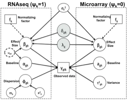
Here we assume that the raw RNA-seq count values follow a negative binomial distribu-tion under each condidistribu-tion. We also assume that genes are matched across studies. Although the model could be readily extended to analyze multiple studies with similar but not com-pletely overlapped gene sets. In the next three subsections, we will introduce the generative model within each study (Section2.2.2), describe information integration of effect sizes across studies (Section2.2.3) and model clusters of genes with different DE patterns across studies (Section 2.2.4). Figure 2 provides a graphical representation of the full Bayesian hierarchi-cal model. Parameters within the rectangle form the main model and parameters outside the rectangle are hyperparameters. The gray shaded parameters δgk (latent variable of DE
ygik
αgk βgk Observed count φgk Baseline Effect Size Dispersion δgk λg ρ ηg r mg t pc ωgik τ2 σ2 ξ2 πgk cg G0 zgk θc
≡
Figure 2: “BayesMetaSeq”: Graphical representation of the Bayesian hierarchical model
indicator) and λg (DE effect size) are the parameters of interest in the model. The dashed rectangle refers to a Dirichlet process mixture (DPM) model for DE gene categorization that will be described in Section 2.2.4.
2.2.2 Generative model within each study
Below, we describe the generative model for observed data within each study. We assume the counts ygik, conditioning on hyperparameters, are independent and follow a negative binomial distribution. Denote by µgik = E(ygik) the mean expression level and φgk the gene-specific dispersion parameter, we have:
ygik ∼N B(µgik, φgk). (2.2.1) We then fit a log-linear regression model for the meanµgik, whereαgkdenotes the baseline expression relative to the library size andβgk denotes the effect size (i.e. the log fold change
of expression between the two conditions):
log(µgik) = log(Tik) +αgk+βgkXik. (2.2.2) Note that we setβgk to depend on bothg and k, allowing the existence of between study heterogeneity for the same gene. If we re-parametrize the negative binomial model in (2.2.1) in terms of proportion p (≡ 1+φµφµ) and dispersion φ, and let Ψ = logit(p) = log(
φµ
1+φµ
1
1+φµ
) = log(φµ), we can re-write equation (2.2.2) as:
Ψgik = log(Tik) +αgk+βgkXik+ log(φgk). (2.2.3) The above equation is useful when we later use Gibbs sampling to update the parameters
αgk and βgk. Taking equation (2.2.1) and (2.2.2) together form our basic GLM model as follows:
ygik|αgk, βgk, φgk ∼N B(log(Tik) +αgk+βgkXik, φgk). (2.2.4)
2.2.3 Information integration of effect size across studies among DE genes Next, we select appropriate prior distributions for the model parameters in equation (2.2.4) to allow information integration across studies. We first define the following vectors:
~
αg = (αg1, . . . , αgK)T, β~g = (βg1, . . . , βgK)T, log(φ~g) = (log(φg1), . . . ,log(φgK))T, which represent the baseline, effect size and dispersion vectors for gene g respectively. The three vectors are assumed to be a priori independent of each other. In addition, we define the vector for the differential expression indicators of gene g: ~δg = (δg1, . . . , δgK)T. We assume each of the vectors α~g,logφ~g follows a multivariate Gaussian distribution:
~
αg ∼NK(ηg,Λ), logφ~g ∼NK(mg,Π), (2.2.5) where ηg and mg are the gene-specific grand means for ~αg and logφ~g, respectively. The covariance matrices Λ and Π are shared by all genes to be described below. For β~g, we assume a multivariate Gaussian prior, with different means for DE and Non-DE genes:
~
whereλg is the gene-specific grand mean for DE genes (i.e. δgk 6= 0 for some k). For Non-DE genes (~δg = 0), the grand mean is 0. We also allow a different covariance matrix of β~g for DE and Non-DE genes, i.e. Σ=Σ1 for DE genes and Σ=Σ0 for Non-DE genes.
Adopting the separation strategy on modelling covariance matrices by Barnard et al.
(2000), we propose independent prior distributions on the diagonal variance components and the off-diagonal correlation matrix for all the four covariance matrices mentioned above. Let [ρ(1)kk0]K 1 , [ρ(0)kk0] K 1 , [rkk0] K 1 and [tkk0]K
1 denote the correlation matrices corresponding
to the covariance matrices Σ1, Σ0, Λ and Π respectively, and let [σ2(1),k] K 1 , [σ 2 (0),k] K 1 , [τ2k] K 1 and [ξ 2 k] K
1 denote the corresponding diagonal matrices with the variance terms on
the diagonal. It is widely known that:
Σ1 = ([σ2(1),k] K 1 ) 1/2 [ρ(1)kk0]K 1 ([σ 2 (1),k] K 1 ) 1/2 , Σ0 = ([σ2(0),k] K 1 ) 1/2 [ρ(0)kk0] K 1 ([σ 2 (0),k] K 1 ) 1/2 , Λ= ([τ2k] K 1 ) 1/2 [rkk0]K 1 ([τ 2 k] K 1 ) 1/2 , Π= ([ξ2k]K1 )1/2[tkk0]K 1 ([ξ 2 k] K 1 ) 1/2 .
For each variance component, we propose a Jeffrey’s prior, that is to say:
σ2(1),k ∝ 1 σ2 (1),k , σ(0)2 ,k ∝ 1 σ2 (0),k , τk2 ∝ 1 τ2 k , ξk2 ∝ 1 ξ2 k .
For the correlation matrices, we propose an inverse-Wishart prior distribution with identity matrix as its scale matrix and v =K+ 1 degrees of freedom, which is equivalent to putting a uniform prior on each element of the correlation matrices marginally (Gelman et al.,2014;
Scharpf et al., 2009; Barnard et al., 2000), more specifically we have:
[ρ(1)kk0]K 1 ,[ρ(0)kk0] K 1 ,[rkk0] K 1 ,[tkk0] K 1 ∼W −1(I, v).
For gene-specific grand means λg, ηg and mg, we assume that they follow normal priors, e.g. λg ∼N(µλ, σλ2), ηg ∼ N(µη, ση2), mg ∼ N(µm, σm2 ) with mean µλ = 0, µη = 0, µm = 0, and variance σ2
λ = 102, σ2η = 102, σ2m = 102. We performed sensitivity analysis on the hyperparameter values, since the varianceσλ2,σ2ηandσ2mare fairly large, the results show little
change when the means µλ, µη and µm change (see Appendix for the result of a sensitivity analysis on hyperparameter µη).
In addition to the informative parameters listed above, we introduce one supporting parameter ωgik into the model to help obtain closed-form posterior distribution for βgk and
αgk by exploiting conditional conjugacy (Polson et al.,2013; Zhou et al., 2012b). The prior for ωgik is specified as:
ωgik ∼P G(ygik +φ−gk1,0),
where PG refers to the Polya-Gamma distribution, details about this distribution and how the supporting parameter facilitates conditional conjugacy are provided in the Appendix. The closed-form posterior distribution for βgk and αgk by conditional conjugacy speeds up MCMC simulation.
2.2.4 Model-based clustering to categorize DE genes
We next utilize the differential expression indicators δgk to cluster the DE genes and model the homogeneous and heterogeneous differential signals across studies. Since clustering based on the binary latent variable is unstable and does not take effect size into consideration, we first transform the binary vector into a standard normal vector and use Dirichlet process Gaussian mixture model to cluster the DE genes, followingMedvedovic et al.(2004). Suppose
P(δgk = 1) =πgk is the prior probability that a geneg is DE in studyk, the effect size is used to turnπgk into a signed probability measure π±gk =πgk×sign(βgk) where sign(.) is the sign function. We further rescale πgk∗ = (π±gk+ 1)/2, so the score falls in the range [0,1]. Lastly, we transform πgk∗ to a Z-score zgk = Φ−1(π∗gk) where Φ is the standard normal cumulative distribution function. Following Ferguson (1983) and Neal (2000), we construct a Dirichlet process mixture (DPM) framework to cluster the DE genes:
~ zg|cg,θ ∼F(~θcg), P(cg =c) =pc, ~ θc∼G0, ~
p∼Dirichlet(a/C, . . . , a/C).
where~zg = (zg1, . . . , zgK)T andcgindicates the “latent cluster” for geneg,F(.) is a mixture of
K-dimensional multivariate Gaussian distributions with mean~θcand covariance matrix being identity matrix. Cis the number of clusters, which is stochastic and allowed to go to infinity under DPM. G0 is the base distribution, in this case, G0 =NK(~0,I) and ~p= (p1, . . . , pC) is the mixing proportions for the clusters. a/C is the concentration parameter. In our model, we specify a =C so the marginal prior distribution of each mixing proportion pc would be Unif(0,1) under the constraint
C P c=1
pc= 1.
The above descriptions fully define the hierarchical Bayesian model proposed. The ob-served data are the raw counts, the library size and the phenotypic indicator {ygik, Tik, Xik}, the parameters we need to update through sampling includeδgk,βgk,αgk,φgk,λg,ηg,mg,σk2,
τ2
k,ξk2,ρkk0,rkk0,tkk0,ωgik,cg and C. The hyperparameters we prespecify includev =K+ 1,
µλ = 0, µη = 0, µm = 0, σ2λ = 102, ση2 = 102, σ2m = 102 and Cinit = 10.
2.2.5 Simulating posterior distribution via MCMC
We use the Metropolis-Hastings (MH) algorithm (Metropolis et al.,1953;Hastings,1970) as well as the Gibbs sampling algorithm (Geman and Geman,1984) to infer the posterior distri-bution of the parameters. Depending on the form of the distridistri-bution, 5 types of mechanisms are proposed to update the 16 groups of parameters.
1. The full conditional for αgk and βgk are bivariate normal with known ~ωgk. The full conditional for ~ωgk is Polya-Gamma distribution with knownαgk and βgk (Polson et al.,
2013;Zhou et al., 2012b). We use Gibbs sampling to update them sequentially for each gene g in study k.
2. The full conditional for λg, ηg and mg are multivariate Gaussian distribution for each gene g. The full conditional for each element in [σ2k]
K 1 , [τ 2 k] K 1 and [ξ 2 k] K 1 is an
inverse-gamma distribution. The full conditional for [ρkk0]K1 , [rkk0]K
1 and [tkk0]
K
1 are inverse
Wishart distributions. For all the above with closed form conditional distributions, we use Gibbs sampling to update them.