Zhuoqiong (Charlie) Chen, David Ong and Ella Segev
Heterogeneous risk/loss aversion in
complete information all-pay auctions
Article (Accepted version)
Refereed
Original citation:Chen, Zhuoqiong (Charlie), Ong, David and Segev, Ella (2017) Heterogeneous risk/loss aversion in complete information all-pay auctions. European Economic Review . ISSN 0014-2921
DOI: 10.1016/j.euroecorev.2017.03.002
Reuse of this item is permitted through licensing under the Creative Commons:
© 2017 Elsevier B.V. CC BY-NC-ND 4.0
This version available at: http://eprints.lse.ac.uk/70793/ Available in LSE Research Online: March 2017
LSE has developed LSE Research Online so that users may access research output of the School. Copyright © and Moral Rights for the papers on this site are retained by the individual authors and/or other copyright owners. You may freely distribute the URL
Accepted Manuscript
Heterogeneous Risk/Loss Aversion in Complete Information All-pay Auctions
Zhuoqiong (Charlie) Chen, David Ong, Ella Segev
PII: S0014-2921(17)30049-1
DOI: 10.1016/j.euroecorev.2017.03.002
Reference: EER 2969
To appear in: European Economic Review Received date: 23 June 2016
Accepted date: 3 March 2017
Please cite this article as: Zhuoqiong (Charlie) Chen, David Ong, Ella Segev, Heterogeneous Risk/Loss Aversion in Complete Information All-pay Auctions, European Economic Review (2017), doi:
10.1016/j.euroecorev.2017.03.002
This is a PDF file of an unedited manuscript that has been accepted for publication. As a service to our customers we are providing this early version of the manuscript. The manuscript will undergo copyediting, typesetting, and review of the resulting proof before it is published in its final form. Please note that during the production process errors may be discovered which could affect the content, and all legal disclaimers that apply to the journal pertain.
ACCEPTED MANUSCRIPT
Heterogeneous Risk/Loss Aversion in Complete Information
All-pay Auctions
Zhuoqiong (Charlie) Chena, David Ongb, Ella Segevc
aHarbin Institute of Technology, Shenzhen, University Town, Nanshan District, 518055, Shenzhen, China.
London School of Economics, Houghton Street, WC2A 2AE, London, United Kingdom. Email: [email protected]
bCorresponding author. Peking University, HSBC Business School, University Town, Nanshan District,
518055, Shenzhen, China. Email: [email protected]
cBen Gurion University of the Negev, P.O.B 653, 84105, Beer Sheva, Israel. Email: [email protected]
Abstract
We extend previous theoretical work on n-player complete information all-pay auctions to incorporate heterogeneous risk- and loss-averse utility functions. We provide sufficient and necessary conditions for the existence of equilibria with a given set of active players with any strictly increasing utility functions and characterize the players’ equilibrium mixed strategies. Assuming that players can be ordered by their risk aversion (player a is more risk-averse than player b, if whenever player b prefers a certain payment over a given lottery, so does player a), we find that in equilibrium, the more risk-averse players either bid higher than the less risk-averse players and win with higher ex-ante probability – or they drop out. Furthermore, while each player’s expected bid decreases with the other players’ risk aversion, her expected bid increases with her own risk aversion. Thus, increasing a player’s risk aversion creates two opposing effects on total expected bid. A sufficient condition for the total expected bid to decrease with a player’s risk aversion is that this player is relatively more risk-averse compared to the rest of the players. Our findings have important implications for the literature on gender differences in competitiveness and for gender diversity in firms that use personnel contests for promotions.
Keywords: All-pay auction, Risk aversion, Loss aversion
ACCEPTED MANUSCRIPT
1. Introduction
Sunk cost contests, where effort is unrecoverable, are pervasive (Frank and Cook, 2010). All-pay auctions are those where the winners need only exert slightly higher effort to take all. Indeed, all-pay auctions theory has been used to study many types of sunk cost contest and tournaments, e.g., rent seeking contest and lobbying (Baye et al., 1993; Ellingsen, 1991; Hillman and Riley, 1989), election campaigns (Che and Gale, 1998), R&D races (Dasgupta et al., 1982), curved grades (Andreoni and Brownback, 2014), college admission (Hickman, 2014), and job promotion (Rosen, 1986). In these contests, the risk of lost effort, oppor-tunities, or resources to individuals can be significant. Furthermore, even contests between organizations, like firms, can involve significant loss to individuals to the extent that decisions are made by CEOs and managers who care about the consequences of those decisions on their own welfare through mechanisms such as options in compensation packages (Bertrand, 2009), and of course, in promotions and dismissals based upon relative performance. Het-erogeneous risk aversion (e.g., as indicated by gender) could thus have a significant influence on behavior.
Evidence is accumulating of a gender difference in risk aversion, where women are usu-ally found to be more risk-averse than men (Charness and Gneezy, 2012; Borghans et al., 2009; Croson and Gneezy, 2009). This gender difference emerges even before adolescence (Khachatryan et al., 2015). A gender difference in risk attitude and its interactions with all-pay auction incentives in the business world can help explain the paucity of women among top executives (Bertrand, 2009), particularly in entrepreneurial settings (Coates et al., 2009). However, despite the importance of observable differences in attitude towards risk in such contests, the modeling of all-pay auction incentives has generally been limited to risk neutral players or to specific tractable utility functional forms.
In order to fill the gap in the theory of all-pay auctions, we extend Baye, Kovenock, and De Vries’s (1996) n-player, complete information all-pay auction model to incorporate heterogeneous risk-averse players. We provide sufficient and necessary conditions for an equilibrium with a given set of active players to exist and more importantly, closed-form solutions to the equilibrium strategies for any strictly increasing utility functions. Assuming
ACCEPTED MANUSCRIPT
b, if whenever player b prefers a certain payment over a given lottery, so does player a), we derive novel comparative statics for equilibria in which active players randomize continuously from 0 to the common value of the prize.
We find that, in equilibrium, the more risk-averse players either bid higher than the less risk-averse players (in terms of first-order stochastic dominance of their mixed strategy cumulative distribution) and win with higher ex-ante probability – or they drop out. When players are homogeneous in their risk aversion, the total expected bid decreases with their risk aversion. We also find, in the heterogeneous risk aversion case, that while each player’s expected bid decreases with the other players’ risk aversion, her expected bid increases with her own risk aversion. Thus, increasing a player’s risk aversion creates two opposing effects on total expected bid. A sufficient condition for the total expected bid to decrease with a player’s risk aversion is that this player is relatively more risk-averse compared to the rest of the players.
Our findings have important implications for the gender differences in competitiveness literature. With only two risk aversion types of players, e.g., men and women, we show that the total expected bid decreases monotonically with the share of the more risk-averse players, when the difference between the two types is not too large. Moreover, our findings suggest the possibility that if women are more risk-averse than men, they can simultaneously work harder than men and decrease everyone’s effort in the firm in personnel contests that have an all-pay auction structure. In these contests, if men and women are not too different in their levels of risk aversions, then a higher share of women may lead to increased odds of a specific woman dropping out. We discuss the specific results in the gender differences in competitiveness literature that these findings can help explain after the main results.
1.1. Literature review
As is always the case with equilibria of complete information all-pay auctions with more than two players, there is no uniqueness of the equilibrium. In fact, there is a continuum of equilibria as in Baye et al. (1996); Siegel (2009); Barut and Kovenock (1998), and Hillman and Samet (1987). Some of the active players may be randomizing over a sub-interval of the form [b, v]. As is the case with risk neutral players, these b’s are arbitrary. Varying the
ACCEPTED MANUSCRIPT
b’s and the set of active players generates the continuum of equilibria. We generalize Baye et al. (1996) equilibrium strategies for risk/loss-averse players. We also generalize Chen et al. (2015) from two players with heterogeneous risk aversion to n players.
Siegel (2009) studies a very general environment that also allows for risk-averse players.
However, his “power condition” for a generic contest does not hold in our environment. The power of a player (in our setting) is defined as her utility at zero. The power condition states that only one of the players has a power of zero. However, if we assume that the utility of each player is zero at zero, then all players have a power of zero, and the condition is violated. If we do not make this assumption, then our model does not comply with Assumption 2 in Siegel (2009). In either case, we cannot use his results to identify all the equilibria of our all-pay auction. When players are homogenous in their risk aversion, we can conclude from Corollary 3 in Siegel (2009) that all the equilibria are of the form that we find in this paper. Hillman and Samet (1987) also solve for an equilibrium with risk-averse players when all players are homogenous in their risk aversion. They characterize the unique symmetric equilibrium in mixed strategies and show that in the presence of risk aversion, rent dissipation is incomplete. Our results characterize all the equilibria for homogenous risk aversion players.
For incomplete information (private value) all-pay contests, Fibich et al. (2006) show that risk aversion has different effects on different types of players. Low value types bid lower and high value types bid higher than they would bid in the risk neutral case. Moreover, they show, as we do, that the seller’s expected payoff in the risk-averse case may be either higher or lower than in the risk neutral case.
Parreiras and Rubinchik (2010) analyze pure strategy equilibrium with heterogeneous risk-averse players, also in an incomplete information setting. They allow for heterogeneity in both the risk preferences and the supports of the distributions from which the private values are drawn. Our model can be thought of as a limiting case of their model when all supports contain only one point (the same for all players). Thus, our results often echo theirs. First, Parreiras and Rubinchik (2010) characterize conditions for a given set of players to be active on a given support, as we do. Moreover, they show that with at least three heterogeneously risk-averse contestants, some might drop out either partially or completely.
ACCEPTED MANUSCRIPT
This is identical to our mixed strategy equilibria of the complete information (common value) case where some players may randomize on a sub-interval of the interval from zero to the common value, and some players may drop out completely. They also show, as we do, that more risk-averse players are more aggressive in their bidding in terms of first-order stochastic dominance of the bid function, at least in some neighborhoods of zero and of the highest bid. Most importantly, they show that with two types of risk aversions, if the risk-averse players are sufficiently risk-risk-averse, then in any equilibrium, at least one contestant uses a discontinuous strategy: a mass of low valuation types drops out from the contest, high valuation types place high bids, but no types place low bids. This gives rise to bid bifurcation, where only bids at zero or bids above a threshold are observed for some players. Analogously, in our setting a player may randomize continuously on a sub-interval [b, v] for some b > 0 (where v is the common value) and put a positive mass on bidding zero. The main difference between the papers is that in our complete information setting, we are able to analytically derive the bid functions while Parreiras and Rubinchik (2010) characterize only some of its properties. This allows us to derive results on the behavior of players with different risk attitudes and comparative statics on different aspects of the model.
Klose and Schweinzer (2014) analyze incomplete information all-pay auctions with sym-metric variance-averse players. They assume a specific utility function which is increasing in the player’s expected payoff and decreasing in the variance of the payoff. They characterize the equilibrium bid functions and show that variance aversion is a sufficient assumption to predict that high-valuation players increase their bids relative to the risk-neutral case while low types decrease their bid.
2. The model
There are m players who have a common valuation, v1 = · · · = vm = v for the prize1.
Denote by M the set of players. Players compete in an all-pay auction for one prize by submitting a bid (exerting an effort): xi. The vector of bids is denoted (x1, x2, . . . , xm). The
1Our model can be trivially extended to the case in which one player has a higher valuation, while all other players have the same lower valuation. However, when there are finite many possible valuations, the interaction between valuation and risk attitude significantly complicates the model. We leave this for future work.
ACCEPTED MANUSCRIPT
payoff function in an all-pay auction is given by:
πi(x1, x2, . . . , xm) = −xi if ∃j, xj > xi v−xi if xj < xi for all j .
Moreover, there exists some tie-breaking rule to determine the winner in case there is more than one player with the highest bid. Any tie-breaking rule is applicable in our model. We assume that players are risk/loss-averse with strictly increasing utility functions which we denote by U1(x), U2(x), . . . , Um(x). These utilities are common knowledge and potentially
different from each other. We discuss two cases separately: 1) risk-averse and 2) loss-averse. For case 1), we assume only continuity and concavity of the strictly increasing utility functions. For case 2), we assume that the utility functions take the following form:
Ui(x) = gi(x) if x >0 0 if x= 0 li(x) if x <0 , (1)
where the utility from gains, gi(x) is a strictly increasing concave function while the utility
from losses, li(x) is a convex function, and both are continuous in their domains.
In this paper, we focus on mixed strategy equilibria. In any such equilibria, any active player (a player who bids a positive amount with positive probability)iis indifferent between all the bids in her equilibrium support. Formally, that means,
ρUi(v−x) + (1−ρ)Ui(−x) =Ui(CEi(x, b−i)), (2)
wherexis in the support of the player’s equilibrium strategy,ρdenotes the probability that playeriwins when she bidsx, andCEi(x, b−i) is the certainty equivalent of biddingxgiven
the other players bid b−i. We can rewrite equation (2) as:
Pr(i wins|x, b−i) =ρ=
Ui(CEi)−Ui(−x)
Ui(v−x)−Ui(−x)
ACCEPTED MANUSCRIPT
We defineKUi(x) to facilitate the analysis of the mixed strategy equilibria:
KUi(x) =
Ui(0)−Ui(−x)
Ui(v−x)−Ui(−x)
.
Note thatKUi(x) is strictly increasing inxwith KUi(0) = 0 andKUi(v) = 1. In our analysis
of equilibria, we examine equilibria with the same structure as in Baye et al. (1996) in which all players have v in the support of their equilibrium mixed strategy and no player has an atom at v. In this case, bidding v yields a certain payoff of zero. Therefore, each player is indifferent between any bid in her support and a certain payoff of zero. The equilibrium probability of winning that makes playeri indifferent between bidding x > 0 and receiving a certain payoff of zero is equal toKUi(x). We sometimes abuse notation and write KUi(x)
as Ki(x), and we refer toKi(x) as player i’s “contest risk preference” for reasons below.
In what follows, we exploit the following important property of KUi(x). Its magnitude
depends only on player i’s risk attitude and not on any other players’ risk attitude or bids. As is usually the case with mixed-strategy equilibria, since KUi(x) denotes the probability
that player i wins by submitting a positive bid x, this probability is pinned down by the preferences of player i alone. We show that KUi(x) is monotonic in player i’s risk aversion
in the lemma below. All proofs are in the Appendix. We first define increasing risk aversion and increasing loss aversion.
Definition 1 A concave utility function U(·) represents a more risk-averse player than the concave utility functionU˜(·),if for any lotteryl over a set of prizesZ, the lottery’s certainty equivalent is smaller under U than under U˜. In that case, we say that the risk aversion of the player increases from U˜ to U.
Definition 2 For a player with a utility functionU(·) of the form (1), a convex loss-averse functionl(·)represents a more loss-averse player than the convex function˜l(·),ifl(x)<˜l(x)
for all x <0.
Lemma 1 If Ui(x) is concave, then for any x∈(0, v), Ki(x) increases with player i’s risk aversion, i.e., if Ui represents a more risk-averse player than U˜i, then KUi(x)> KU˜i(x) for
ACCEPTED MANUSCRIPT
function of the form (1), then for any x, Ki(x) increases with player i’s loss aversion.Note that Lemma 1 above also suggests that theK(x) function of different players never cross if the players can be ordered by their risk or loss aversions. The following is an example of the contest risk preference function K(x) when the player has CARA utility function:
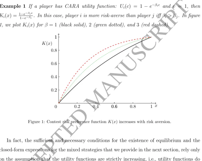
Example 1 If a player has CARA utility function: Ui(c) = 1−e−βic and v = 1, then
Ki(x) = 1−e −βix
1−e−βi . In this case, playeri is more risk-averse than playerj iffβi> βj. In figure 1, we plot Ki(x)for β= 1 (black solid), 2 (green dotted), and3 (red dashed).
1 0.8 0.6 0.4 0.2 0 1 1 0.8 0.6 0.6 0.4 0.2 K(x) x
Figure 1: Contest risk preference functionK(x) increases with risk aversion.
In fact, the sufficient and necessary conditions for the existence of equilibrium and the closed-form expressions for the mixed strategies that we provide in the next section, rely only on the assumption that the utility functions are strictly increasing, i.e., utility functions do not have to be rankable by their certainty equivalent. The rest of the results apply to any utility function that is rankable by certainty equivalent, irrespective of whether the utility function is risk-averse, loss-averse, or even risk seeking. All the results with risk-loving players can be derived analogously, as long as the more risk-loving utilities have a higher certainty equivalent than the less risk-loving utilities for every lottery. We focus only on risk- and loss-averse utilities due to their ubiquity in the literature.
ACCEPTED MANUSCRIPT
3. Equilibrium
In this section, we characterize the sufficient and necessary conditions for the existence of an equilibrium with a given structure and a given set of active players, and then, we characterize the mixed strategies in these equilibria. We also highlight some interesting features of the equilibria in the Subsection 3.2. In discussing these features, for simplicity, we focus only on the equilibria in which all active players randomize on the entire interval [0, v].
3.1. Existence and closed-form solution
Our first proposition, Proposition 1 provides the necessary and sufficient conditions for the existence of an equilibrium in which a given subset of players is active. We start by defining an active player.
Definition 3 A player is active when she bids zero with a probability strictly less than 1. A player is inactive when she bids zero with probability 1.
Denote the set of active players byB ⊆ {1, . . . , m}. For convenience and without loss of generality, we assigni= 1,2, ...,|B|as the index for the active players. Denote byGi(x) the
CDF of player i’s mixed strategy and by αi(0) the mass player i puts on the bid zero. The
equilibrium of the all-pay auction, has the following structure (as with risk neutral players):
1. Playersi= 1,2, . . . , h, where 26h6|B|, randomize continuously over [0, v] and have αi(0) = 0;
2. Playersi=h+ 1, h+ 2, . . . ,|B| randomize continuously over [bi, v] and put a mass of
αi(0) at zero, with 0 =bh < bh+1 6bh+26. . .6b|B| 6b|B|+1=v;
3. Playersj =|B|+ 1, . . . , m are inactive, i.e., αj(0) = 1.
Baye et al. (1996) showed that there is a continuum of equilibria, as the parameters bh+1, bh+2, . . . , b|B| can be chosen arbitrarily, and these determine the size of αi(0). We
now characterize the equilibrium strategy with the same structure but with heterogeneous risk/loss-averse players.
In our setting, this implies that playeri’s (∀i∈B) expected utility must be equal toUi(0)
ACCEPTED MANUSCRIPT
randomize in the interval [bt, bt+1]. Thus, for player i 6 t and ∀x ∈ [bt, bt+1], we have in
equilibrium: Y l6=i,16l6t Gl(x) Y t<l6|B| αl(0) Ui(v−x)+ 1− Y l6=i,16l6t Gl(x) Y t<l6|B| αl(0) Ui(−x) =Ui(0). (3)
Recall thatGl(x) is the probability playerl6=ibids lower thanx, andαl(0) is the probability
that player l bids zero, so Ql6=i,16l6tGl(x)Qt<l6|B|αl(0) is player i’s probability of winning
when biddingx. Thus
Y l6=i,16l6t Gl(x) Y t<l6|B| αl(0) =Ki(x).
We solve this system oft equations and get the equilibrium strategy of playeri6t:
Gi(x) = Q l6=i,16l6tKl(x) Q t<l6|B|αl(0) ! 1 t−1 Ki(x)− t−2 t−1, (4)
wherei6tand x∈[bt, bt+1]. Recall that for player t we haveαt(0) =Gt(bt). By a similar
procedure, we can characterize the entire equilibrium:
• Forx∈[b|B|, v] Gi(x) = Y 16l6|B| Kl(x) 1 |B|−1 Ki(x)−1, (5) wherei= 1, . . . ,|B|.
• Fort=h+ 1, h+ 2, . . . ,|B| −1, we have for x∈[bt, bt+1]
Gi(x) = Q 16l6tKl(x) Q t<l6|B|αl(0) ! 1 t−1 Ki(x)−1, (6) wherei= 1,2, . . . , t; and Gk(x) =αk(0), (7)
ACCEPTED MANUSCRIPT
wherek=t+ 1, . . . ,|B|. • Finally, forx∈[0, bh+1] Gi(x) = Q 16l6hKl(x) Q h<l6|B|αl(0) ! 1 h−1 Ki(x)−1, (8) wherei= 1,2, . . . , h; and Gk(x) =αk(0), (9) wherek=h+ 1, . . . , m.There are three sets of constraints to ensure that the above strategy profile is indeed an equilibrium. First, the players who do not bid somex∈[bt, bt+1] in equilibrium must find it
unprofitable to do so; Second, the players who bidx ∈[bt, bt+1] in equilibrium must have a
feasible CDF at x, i.e., between zero and one; Third, all the CDFs must be non-decreasing in x.
To find the first set of constraints, we first calculate the probability of winning of a player j,for t < j 6|B|who deviates to a bid x∈[bt, bt+1]:
Y 16i6t Gi(x) Y t<l6|B|,l6=j αl(0) = Y i6t Q 16l6tKl(x) Q t<l6|B|αl(0) ! 1 t−1 Ki(x)−1 Q t<l6|B|αl(0) αj(0) = Q 16l6tKl(x) Q t<l6|B|αl(0) ! 1 t−1 1 αj(0) . Thus, we need Y 16i6t Gi(x) Y t<l6|B|,l6=j αl(0)6Kj(x) or Q 16l6tKl(x) Q t<l6|B|αl(0) 6(αj(0)Kj(x))t−1 (10)
to guarantee that player j finds it unprofitable to bid x∈[bt, bt+1], as Kj(x) is the required
ACCEPTED MANUSCRIPT
0 for sure. Note that if j is inactive, |B| < j, then αj(0) = 1. We refer to this set of
constraints as theIncentive Constraints.
We find the second set of constraints by restricting the Gi(x) given by (6) to satisfy
Gi(x)61 for all i6t andx∈[bt, bt+1]2:
Q
16l6tKl(x) Q
t<l6|B|αl(0) 6
Ki(x)t−1. (11)
We refer to this set of constraints as theFeasibility Constraints. Combining the two sets of constraints, (10) and (11), we have:
Q 16l6tKl(x) Q t<l6|B|αl(0) 6 min min 16i6tKi(x) t−1, min t<j6m[αj(0)Kj(x)] t−1 , (12)
for all t=h, h+ 1, . . . ,|B|, and for allx∈[bt, bt+1].
The third set of constraints are derived by ensuring that the first-order derivatives of Gi(x) for all x∈[bt, bt+1] are non-negative in the interval. Since
dGi(x) dx = Q 16l6tKl(x) Q t<l6|B|αl(0) ! 1 t−1 1 (t−1)Ki(x) t X l=1,l6=i Kl0(x) Kl(x) − (t−2)Ki0(x) Ki(x) ! , the constraint is t X l=1 K0 l(x) Kl(x) > (t−1)Ki0(x) Ki(x) , (13)
for all t=h, h+ 1, . . . ,|B|,i= 1, ..., t andx∈[bt, bt+1].
Proposition 1 An equilibrium with the strategy profile (5)-(9) exists if and only if the con-ditions (12) and (13) are satisfied.
The condition (13) restricts the level of risk/loss aversion of the players who bid in the interval [bt, bt+1], whereas condition (12) imposes restrictions on both active and inactive
players. Intuitively, for an equilibrium to exist, the active players cannot be too averse to risk/loss. See the following example for the importance of these conditions.
2AllG
ACCEPTED MANUSCRIPT
Example 2 Assume there are three players with CARA utility functions Ui(x) = 1−e−βix and a valuation v = 1 for i = 1,2,3. Assume that β3 = 1, β2 = 2, β1 = 10. Then,
there exists no equilibrium in which all three players are active and all randomize con-tinuously on [0,1], since the condition is violated on [0.13035,1]. Specifically, we have
G3(x) = (K1(x)K2(x)) 1 2 K 3(x)− 1 2 = 1−e−2x 1−e−2 1−e −10x 1−e−10 1 2 1−e−x 1−e−1 −1 2
, which is larger than 1 for
x>0.13035. However, there exists an equilibrium in which only players 2 and 3 are active and they randomize continuously on the interval [0,1] according to the following strategies:
G2(x) =K3(x) = 1−e
−x
1−e−1 and G3(x) =K2(x) = 1−e
−2x
1−e−2 , since then, all the conditions hold.
Similar to the risk neutral setting, there is also a continuum of equilibria when players are heterogeneously risk/loss-averse. Unlike in the risk neutral setting, players may stay inactive due to the their higher risk/loss aversion. This fact does not restrict the power of our theory in making predictions either for empirical or experimental data, since in reality we can generally observe the number of active players, especially if players play over multiple rounds.
Unlike the risk neutral setting, even if we focus only on the equilibria in which all active players randomize in the full support [0, v], there always exists multiple equilibria3 (see
Corollary 1 below).
Corollary 1 Suppose all players can be ranked by their risk aversions: K1(x) >K2(x)>
. . .>Km(x)for all x∈[0, v], then there always exists equilibria in which only players i and
m are active, where i∈ {1,2, ..., m−1}and randomize continuously on [0, v].
This corollary follows directly from Proposition 1. Condition (12) is automatically sat-isfied since there are only two active players and one of them is the least risk-averse player, m. Condition (13) is satisfied due to the fact that all contest risk preference functionsK(x) are increasing inx.
3In the risk neutral setting, there exists a unique symmetric equilibrium in which all players fully ran-domize within [0, v]. See Baye et al. (1996) for details.
ACCEPTED MANUSCRIPT
3.2. Some features of equilibriaHere we focus on equilibria in which all active players randomize continuously on [0, v]. Assume that B ={1, ...,|B|}is the active set. Then, the conditions for such an equilibrium to exist are: Y 16l6|B| Kl(x)6 min 16i6mKi(x) |B|−1,
for all x∈[0, v] and
|B| X l=1 K0 l(x) Kl(x) > (|B| −1)Ki0(x) Ki(x) ,
for alli= 1, ...,|B|andx∈[0, v]. In this case, player i’s,i= 1, ...,|B|, equilibrium strategy is given by Gi(x) = Y 16l6|B| Kl(x) 1 |B|−1 Ki(x)−1. (14)
In real life competitions, it is not uncommon for participants to differ in observable characteristics like gender, ethnicity, culture...etc. It is then important to examine whether risk attitudes associated with these characteristics help to explain differences in competitive behavior. For example, women are under-represented in the elites of many competitive industries (Bertrand, 2009), yet women are also more likely to achieve academic success (Angrist et al., 2009; DiPrete and Buchmann, 2013; Fortin et al., 2015)4. Importantly, our
results below are consistent with this empirical evidence.
Corollary 2 If there exists an equilibrium where the set of all active players, B, randomize continuously on the interval [0, v], and these players can be ranked by their risk aversions:
K1(x)>K2(x)>. . .>K|B|(x) for all x∈[0, v], then the cumulative distribution function of player s’s strategy first-order stochastically dominates that of player t for every t > s. In particular, the players’ expected bids have the same ranking as their levels of risk aversion.
Corollary 2 suggests that more risk-averse players bid higher in expectation than less risk-averse players among all active players. Given that the more risk-averse a player is, the higher she bids conditional on her being active in equilibrium, one may expect that her
ACCEPTED MANUSCRIPT
probability of winning is also higher. Corollary 3 indicates that this conjecture is generally but not always true.
Corollary 3 Assume an equilibrium where all active players (in the set B) randomize con-tinuously on the interval [0, v]. For any two active players, s, t ∈ B, player s’s probability of winning is higher or equal to that of player t if Kt(x) dominates Ks(x) in terms of the reverse hazard rate, i.e., Kt0(x)
Kt(x) >
K0
s(x)
Ks(x) for all x∈[0, v].
Note thatKs(x),Kt(x) are also the joint cumulative distributions of opponents’ bids that
playerss andt are competing against (i.e., Πl∈B,l6=sGl(x) =Ks(x)), respectively. Corollary
3 suggests that the more risk-averse player s is, the more likely she is to win the contest compared to playert, if in player t’s view (as measured by Kt(x)) the contest is sufficiently
more competitive (i.e., dominates in terms of reverse hazard rate) than in player s’s view (as measured by Ks(x)). Example 3 below suggests that the CARA utility functions satisfy
the condition given in Corollary 3. In other words, if players have CARA utility functions, then the more risk-averse a player is, the more likely she is to win ex-ante.
Example 3 Suppose player i (∀i ∈ B) has CARA utility function Ui(x) = 1−e−βix and
v = 1, thus, she has Ki(x) = 1−e −βix
1−e−βi . Take the derivative of Ki0(x)/Ki(x) w.r.t. βi, we have
∂Ki0(x) Ki(x) ∂βi =− e− βix (e−βix−1)2 e −βix+β ix−1 <0.
The above derivative is negative because e−βix+β
ix−1
increases inx, its derivative w.r.t.
x is positive for ∀x∈(0,1], and it is equal to 0 whenx= 0.
Interestingly, the more risk-averse players not only bid higher and win with higher prob-ability, they are also more likely to drop out in the following sense.
Corollary 4 Assume an equilibrium where all active players (in the set B) randomize con-tinuously on the interval [0, v]. If for some i∈B and j /∈B, we have Ki(x)>Kj(x)for all
x ∈[0, v], then the existence of the equilibrium with the set B of active players implies the existence of another equilibrium with the setBe of active players who randomize continuously on the interval [0, v], where Be= (B∪ {j})\ {i}.
ACCEPTED MANUSCRIPT
Corollary 4 suggests that the conditions for the existence of the equilibrium in which a relatively more risk-averse player bids actively is sufficient for the existence of the equilibrium in which a less risk-averse player bids actively, holding all other active and inactive players constant, but the opposite is not necessarily true. This implies that mere differences in risk attitudes can result in different non-entry/drop out decisions, without having heterogeneity in valuations or incomplete information. The player with the higher risk aversion may not participate in the competition because she finds that the potential return from bidding any positive amount does not sufficiently compensate her for the risk.
One implication of this finding is that the well established gender difference in risk aver-sion alone may be sufficient to explain differences in participation rates found in gender differences in competitiveness experiments (Niederle and Vesterlund, 2007)5, without the
need to hypothesize gender differences in competitiveness, confidence, or other characteris-tics.
A question naturally follows: are the players who drop out always those who are more risk-averse than the active ones? The answer is not necessarily. Example 4 suggests there might exist equilibria in which players with the intermediate risk aversion drops out.
Example 4 Assume there are three players with CARA utility functions Ui(x) = 1−e−βix and a valuation v = 1 for i= 1,2,3. Assume also that β1 = 2, β2 = 1, β3 = 12. Then, there
exists an equilibrium in which only players1and3are active, while player2is inactive. The conditions for this equilibrium to exist are:
K1(x)K3(x) = 1−e−2x 1−e−2 1−e−1 2x 1−e−12 6 min{K1(x), K2(x), K3(x)}=K3(x) = 1−e−1 2x 1−e−12
and that theGi(x)functions are strictly increasing for players1and3, which follows directly fromK1(x)andK3(x)being increasing functions. Thus, there exists an equilibrium in which
the most and the least risk-averse players are active while the player with the intermediary risk aversion is inactive.
5These papers examine entry into what are in effect all-pay auctions to measure gender differences in competitiveness. See Niederle (2014) for a recent survey.
ACCEPTED MANUSCRIPT
4. Comparative statics
We now discuss the effect of increasing players’ risk aversion on their expected bids. Our results in this section are derived for the equilibrium in which all active players randomize continuously in [0, v]. Subsection 4.1 shows that if players are homogeneous in their risk attitude, then increasing all players’ risk aversion decreases the total expected bid. Subsec-tion 4.2, in contrast, shows that in the case with heterogeneous risk aversion, each player’s expected bid increases with her own risk aversion, though it still decreases with other active players’ risk aversions.
4.1. Homogeneous risk aversion
The equilibrium strategy with homogeneous risk aversion is a special case of the equi-librium strategy with heterogeneous risk aversion derived above. When players are homo-geneous in their risk aversion, we can generalize the proof of Baye et al. (1996) and prove that all equilibria are of the form described in Proposition 16. In this case, there is a unique
symmetric equilibrium in which all players randomize continuously on [0, v], as well as many asymmetric equilibria. We, again, focus on equilibria in which all active players random-ize on the interval [0, v]. We first examine how the players’ behavior change when they all become more risk-averse.
Proposition 2 Assume all players are homogeneous, then there exists an equilibrium where a set B of players randomize continuously on the interval [0, v], and all other players are inactive. If all the players’ risk aversion increases homogeneously, then their bids in the equilibrium in which the same set B of players randomize continuously on the interval [0, v]
decrease in terms of first-order stochastic dominance.
We illustrate Proposition 2 with the following example.
Example 5 Assume there are three players, each with the CARA utility function: Ui(x) =
1−e−βx and valuation v = 1. Figure 2 shows the unique symmetric equilibrium strategy whenβ= 1(black solid), 5(green dotted), and 10(red dashed). It is clear that as all players
ACCEPTED MANUSCRIPT
become more risk-averse, the distribution function of their bids decreases in terms of first-order stochastic dominance, i.e., the probability that they bid below x for any x ∈ [0, v] is higher when they are more risk-averse. The total expected bid decreases from 0.812to 0.357and then to 0.184. 1 0.8 0.6 0.4 0.2 0 1 1 0.8 0.6 0.6 0.4 0.2 G(x) x
Figure 2: Homogeneously increasing all players’ risk aversion decreasesG(x).
In the complete information all-pay auction with homogenous risk-averse players, the total expected bid, therefore, decreases in the players’ risk aversion. As all players become more risk-averse, they require better odds of winning in order to be compensated for the same risk. To maintain each others’ indifference conditions, as required by equilibrium, all players bid lower in the sense of first-order stochastic dominance, in order to compensate each other for the greater disutility of risk.
4.2. Heterogeneous risk aversion
In this section, we first show in Proposition 3 that each player’s expected bid increases with her own risk aversion, but decreases with other active players’ risk aversions. Given this result, we characterize the sufficient condition for the total expected bid to decrease when the more risk-averse player becomes even more risk-averse in Proposition 4. We again assume that players can be ordered according to their risk aversion. Without loss of generality, let K1(x) > K2(x) > . . . > Km(x) for all x ∈ [0, v], so that player 1 is the most risk-averse
ACCEPTED MANUSCRIPT
Proposition 3 Assume there exists an equilibrium where a set B of players randomize con-tinuously on the interval [0, v] and all other players are inactive. Assume, furthermore, that the level of risk aversion for some player i ∈ B has increased, i.e., Ki(x) changes to
˜
Ki(x) > Ki(x) for every x ∈ [0, v]. Assume that after this change, there still exists an equilibrium where the set B of players randomize continuously on the interval [0, v],and all other players are inactive. Then, the expected bid of player i increases with her level of risk aversion, while the expected bid of player k for k∈B, k 6=idecreases with player i’s level of risk aversion.
The following example illustrates this result.
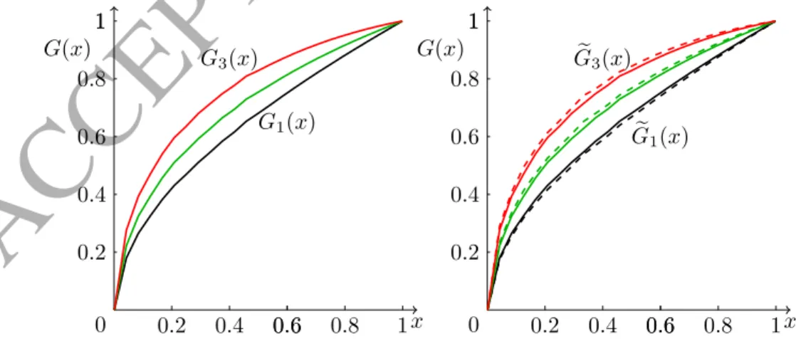
Example 6 Assume there are three players with CARA utility functions Ui= 1−e−βic with
β1= 1, β2 = 0.5, β3 = 0.1 and valuationv = 1for i= 1,2,3. Then, player1is the most risk
averse and K1(x)>K2(x)>K3(x) for all x∈[0,1]. In the equilibrium in which all three
players are active and randomize continuously on the interval[0,1], the equilibrium strategies of the players (the CDFs of their mixed strategies) are given in the left panel of figure 3: G1(x)
(black) 6G2(x) (green) 6G3(x) (red). Assume now that β1 changes to β˜1 = 1.2, then the
players strategies change to the dashed lines as in the right panel of figure 3. It can be seen that player 1’s mixed strategy (black) increases to Ge1(x)6 G1(x) while players 2’s (green)
and 3’s (red) mixed strategy decreases to Ge2(x)>G2(x) and Ge3(x)>G3(x) in the sense of
first-order stochastic dominance, respectively. 1 0.8 0.6 0.4 0.2 0 1 1 0.8 0.6 0.6 0.4 0.2 G(x) x G3(x) G1(x) 1 0.8 0.6 0.4 0.2 0 1 1 0.8 0.6 0.6 0.4 0.2 G(x) x e G3(x) e G1(x)
ACCEPTED MANUSCRIPT
Next, we discuss the effect of a change in the risk attitude of an active player on the total expected bid in equilibrium. We first interpret the intuition behind Proposition 3. In a mixed strategy equilibrium, any active playert is made indifferent between any of his bids by the strategies of the other players. When playertbecomes even slightly more risk-averse, the other players have to lower their bids to ensure player tstays indifferent (in order for an equilibrium with the same set of active players to continue to exist). Thus, by equilibrium strategy (4), increasingt’s risk aversion has two effects on total expected bid, fixing the same set of active players:
1. Playertbids higher, since the CDF of her new equilibrium strategy first-order stochas-tically dominates the CDF of her original equilibrium strategy, before she became more risk-averse;
2. The rest of the players bid lower when Kt(x) increases, since their CDFs decrease in
the sense of first-order stochastic dominance.
The net effect on total expected bids is not obvious. We provide in Proposition 4 a sufficient condition for the total expected bid to decrease when one player’s risk aversion increases, assuming the equilibrium with the same set of active players still exists after the increase of the player’s risk aversion.
Proposition 4 Assume an equilibrium with a set B of active players who randomize con-tinuously on the interval [0, v]. For an active player i, if
Ki(x)> |
B| −2
P
l∈B,l6=iKl(x)−1
, (15)
for all x∈[0, v], then the total expected bid decreases in i’s risk aversion.
Note that the r.h.s. of (15) can be rewritten as the harmonic mean of theK(x) functions of the rest of the active players multiplied by a constant:
|B| −2 P l∈B,l6=iKl(x)−1 = P |B| −1 l∈B,l6=iKl(x)−1 |B| −2 |B| −1.
ACCEPTED MANUSCRIPT
of the active players to guarantee that an increase in her risk aversion decreases the total expected bid. See example 7 for an illustration of Proposition 4.
Example 7 Assume there are three players B ={1,2,3} who have CARA utility functions with β1 = 2, β2 = 1, β3 = 21, and valuation v = 1. Then, K1(x) = 1−e
−2x 1−e−2 , K2(x) = 1−e −x 1−e−1, and K3(x) = 1−e −12x
1−e−12 . Note that the condition (15) for i= 1is satisfied:
K1(x) = 1−e−2x 1−e−2 > 1−e−12 1−e−12x + 1−e− 1 1−e−x !−1 = K2(x)−1+K3(x)−1 −1
and the total expected bid in the equilibrium in which all three players are active and ran-domize continuously on [0,1] is:
3− Z 1 0 (K2(x)K3(x)) 1 2(K 1(x))− 1 2 dx− Z 1 0 (K1(x)K3(x)) 1 2 (K 2(x))− 1 2 dx − Z 1 0 (K1(x)K2(x)) 1 2 (K 3(x))− 1 2 dx= 0.779.
Assume now that we increase player 1’s risk aversion to β1 = 3, then the total expected bid
decreases to 0.723.
Many real-life competitions are composed of participants with evidently different risk attitudes, e.g., mixed gender contests. We now analyze how the risk attitude composition of contests with two different risk types affects participation. Formally, assume there are two sets of contestants in the competition: type 1 players with the contest risk preferenceK1(x),
and type 2 players with the contest risk preferenceK2(x). There aremplayers in total. Let
n be the number of type 1 players, with n < m. All players have the same valuation v for the prize and K1(x) > K2(x) for all x ∈ (0, v). Type 1 players are thus more risk-averse
than type 2 players.
Corollary 5 For any m1 6 mn 61, there exists an equilibrium in which all players randomize continuously on the interval [0, v]if and only if
ACCEPTED MANUSCRIPT
for all x∈[0, v].Corollary 5 establishes that there always exists an equilibrium with all players active for any n
m ∈[0,1], when the inequality (16) is satisfied, i.e., when the more risk averse players are
not too risk-averse compared to the less risk-averse players. Given that such an equilibrium exists, Corollary 6 then provides a sufficient condition for the total expected bid in such an equilibrium to decrease with n
m (the share of the more risk-averse players).
Corollary 6 When there are two risk-averse types of players, with K1(x) > K2(x), for
x∈ (0, v), assume condition (16) in Corollary 5 is satisfied. Then the total expected bid is monotonically decreasing with the share of the K1(x) players, mn, if
K2(x)>
m−2
m−1K1(x). (17)
Corollary 6 explicates the transition in terms of total revenue from the case where all players are homogeneously less risk-averse to the case where all players are homogeneously more risk-averse. As the share of the more risk-averse players increases, the total expected bid decreases monotonically. According to (17), this is true if the two types of players are not too different, as
K1(x)>K2(x)> m−2 m−1K1(x) has to hold. 5. Discussion 5.1. Asymmetric valuation
The literature on complete information all-pay auctions with risk neutral players has traditionally allowed for heterogeneity in valuations of the prize. Here, we compare hetero-geneity in risk aversion to heterohetero-geneity of valuation. Assume two sets of valuations such that vh = v1 = ... = vn > vn+1 = ... = vm = vl and compare to a common value v but
two sets of risk-averse players, i.e., K1(x) = ... =Kn(x) > Kn+1(x) = ....= Km(x) for all
ACCEPTED MANUSCRIPT
First, observe that if n ≥ 2, only the players with the high valuation are active in any equilibrium with risk neutral players and two different valuations. However, in our setting both the more risk-averse players and the less risk-averse players may be active in equilibrium. This phenomena is also true with more types of players. For v1 > v2 > v3 > ... > vm, in
any equilibrium only players 1 and 2 are active while in the risk averse case with K1(x)>
K2(x)> K3(x)>...>Km(x) all players may be active.
Moreover, ifn= 1 then in the risk neutral setting, there exists a continuum of equilibria. In any equilibrium, bidder 1 randomizes continuously on the interval [0, vl]. Each bidder
i, i ∈ {2, ..., m}, employs a strategy Gi with support contained in [0, vl] that has an atom
αi(0) at 0. The size of the atom may differ across bidders, but Πmi=2αi(0) = vhv−lvl. Each Gi
is characterized by a number bi >0, where bi = 0 for at least one i6= 1, such thatGi(x) =
αi(0), for allx∈[0, bi] and bidder irandomizes continuously on (bi, vl]. Furthermore, when
two or more bidders in the set{2, ..., m}randomize continuously on a common interval, their CDFs are identical on that interval. Finally, in any equilibrium bidder 1 earns an expected payoff of vh−vl, while each of the bidders 2, ..., m earns an expected payoff of zero.
In the risk-averse case, we examine equilibria with the feature that all players randomize on an interval contained in [0, v] and may have an atom at zero. This is similar to the risk neutral case where they all randomize on an interval contained in [0, vl] and may have an
atom at zero. However, in our setting all bidders have a payoff of zero in any equilibrium, including the less risk-averse players (the “strong” players). Moreover, weak bidders (more risk-averse) do not necessarily have an atom at zero, while in the risk neutral case, some of them must have an atom so that Πm
i=2αi(0) = vhv−lvl. In the risk-averse setting, it is also
true that when two or more bidders with the same risk aversion randomize continuously on a common interval, their CDFs are identical on that interval.
We can also compare the effects of changes in players’ preferences (i.e., valuation for the prize in the risk neutral case, and risk aversion in the risk-averse case) on the expected total effort. Given an equilibrium of the risk neutral all-pay auction with valuations vl and vh,
and assuming that all bidders randomize on the same interval (starting from the same bi)
before and after the increase, an increase invlnecessarily increases the expected total effort.
ACCEPTED MANUSCRIPT
player may either decrease or increase the expected total effort depending on how much more risk-averse she is than the rest of the players. Therefore, heterogeneous risk aversion gives rise to different predictions on the behavior of the players. These can be empirically tested7.
5.2. Gender difference
Our findings suggest the possibility that the higher risk aversion of women and girls can simultaneously lead them to avoid participating in all-pay auction type incentives while bid-ding higher and having a higher probability of winning than men and boys, when they do participate. Heterogeneous risk aversion, therefore, could be an important factor in explain-ing many of the stylized facts about gender differences in competitiveness, includexplain-ing women’s greater reluctance to enter contests with all-pay auction incentives, like elections, unless they have a good chance of winning (Fulton et al., 2006), girls’ greater willingness to exert effort in preparation (Duckworth and Seligman, 2006) and their higher odds of success in academic contests (Angrist et al., 2009; DiPrete and Buchmann, 2013; Fortin et al., 2015), and women’s greater reluctance to enter laboratory contests (Niederle and Vesterlund, 2007), where they cannot assure themselves success through extra pre-experiment preparation. Moreover, at present, the experimental literature has largely taken for granted that heterogeneous risk aversion is similar to homogeneous in all-pay auction settings in depressing efforts, e.g., that the gender gap in competitiveness decreases when risk aversion is controlled for (Niederle, 2014). Our contribution is to show that this assumption is not warranted and indeed het-erogeneous risk aversion is consistent with many different (and perhaps unexpected) forms of behavior.
Acknowledgments
We would like to thank the anonymous referees and the editor Robert M. Sauer for their very helpful suggestions. We would also like to thank Dan Kovenock, Subhasish M. Chowdhury, Marco Serena, Gahye Jeon, participants of Network for Integrated Behavioral
ACCEPTED MANUSCRIPT
Science Conference, Contest Conference at UEA, and the 5th World Congress of the Game Theory Society for helpful comments. This work was done in part while the third author was visiting the Simons Institute for the Theory of Computing, Berkeley, CA, USA. An earlier version of the paper was included in the first author’s PhD thesis submitted to LSE.
References
Andreoni, J. and A. Brownback (2014). Grading on a curve, and other effects of group size on all-pay auctions. Technical report, National Bureau of Economic Research.
Angrist, J., D. Lang, and P. Oreopoulos (2009). Incentives and services for college achieve-ment: Evidence from a randomized trial. American Economic Journal: Applied Eco-nomics, 136–163.
Barut, Y. and D. Kovenock (1998). The symmetric multiple prize all-pay auction with complete information. European Journal of Political Economy 14(4), 627–644.
Baye, M. R., D. Kovenock, and C. G. De Vries (1993). Rigging the lobbying process: An application of the all-pay auction. American Economic Review 83(1), 289–294.
Baye, M. R., D. Kovenock, and C. G. De Vries (1996). The all-pay auction with complete information. Economic Theory 8(2), 291–305.
Bertrand, M. (2009). CEOs. Annual Review of Economics 1(1), 121–150.
Borghans, L., J. J. Heckman, B. H. Golsteyn, and H. Meijers (2009). Gender differences in risk aversion and ambiguity aversion. Journal of the European Economic Association 7 (2-3), 649–658.
Charness, G. and U. Gneezy (2012). Strong evidence for gender differences in risk taking.
Journal of Economic Behavior and Organization 83(1), 50–58.
Che, Y.-K. and I. L. Gale (1998). Caps on political lobbying. American Economic Re-view 88(3), 643–651.
ACCEPTED MANUSCRIPT
Chen, Z. C., D. Ong, and R. M. Sheremeta (2015). The gender difference in the value of winning. Economics Letters 137, 226–229.
Coates, J. M., M. Gurnell, and A. Rustichini (2009). Second-to-fourth digit ratio predicts success among high-frequency financial traders. Proceedings of the National Academy of Sciences 106(2), 623–628.
Croson, R. and U. Gneezy (2009). Gender differences in preferences. Journal of Economic Literature, 448–474.
Dasgupta, P., R. J. Gilbert, and J. E. Stiglitz (1982). Invention and innovation under alterna-tive market structures: The case of natural resources. Review of Economic Studies 49(4), 567–582.
DiPrete, T. A. and C. Buchmann (2013). The rise of women: The growing gender gap in education and what it means for american schools. Russell Sage Foundation.
Duckworth, A. L. and M. E. P. Seligman (2006). Self-discipline gives girls the edge: Gender in self-discipline, grades, and achievement test scores. Journal of Educational Psychol-ogy 98(1), 198.
Ellingsen, T. (1991). Strategic buyers and the social cost of monopoly. American Economic Review 81(3), 648–657.
Fibich, G., A. Gavious, and A. Sela (2006). All-pay auctions with risk-averse players. Inter-national Journal of Game Theory 34(4), 583–599.
Fortin, N. M., P. Oreopoulos, and S. Phipps (2015). Leaving boys behind. Journal of Human Resources 50(3).
Frank, R. H. and P. J. Cook (2010). The winner-take-all society: Why the few at the top get so much more than the rest of us. Random House.
Fulton, S. A., C. D. Maestas, L. S. Maisel, and W. J. Stone (2006). The sense of a woman: Gender, ambition, and the decision to run for congress.Political Research Quarterly 59(2),
ACCEPTED MANUSCRIPT
Hickman, B. R. (2014). Pre-college human capital investment and affirmative action: A structural policy analysis of US college admissions. University of Chicago, mimeo.
Hillman, A. L. and J. G. Riley (1989). Politically contestable rents and transfers. Economics and Politics 1(1), 17–39.
Hillman, A. L. and D. Samet (1987). Dissipation of contestable rents by small numbers of contenders. Public Choice 54(1), 63–82.
Khachatryan, K., A. Dreber, E. Von Essen, and E. Ranehill (2015). Gender and preferences at a young age: Evidence from armenia.Journal of Economic Behavior and Organization 118, 318–332.
Klose, B. S. and P. Schweinzer (2014). Auctioning risk: The all-pay auction under mean-variance preferences.University of Zurich, Department of Economics, Working Paper (97).
Krishna, V. (2009). Auction theory. Academic press.
Niederle, M. (2014). Gender. InHandbook of Experimental Economics.
Niederle, M. and L. Vesterlund (2007). Do women shy away from competition? Do men compete too much? Quarterly Journal of Economics, 1067–1101.
Parreiras, S. O. and A. Rubinchik (2010). Contests with three or more heterogeneous agents.
Games and Economic Behavior 68(2), 703–715.
Rosen, S. (1986). Prizes and incentives in elimination tournaments. American Economic Review, 701–715.
Siegel, R. (2009). All-pay contests. Econometrica 77(1), 71–92.
6. Appendix Proof of Lemma 1
If player i becomes more risk-averse (from ˜Ui to Ui), then the certainty equivalent of
winningv−x, with probabilityKU˜i(x), and −x, with probability 1−KU˜i(x)
ACCEPTED MANUSCRIPT
zero, which is the certainty equivalent of this gamble with a utility function ˜Ui. Therefore,
the player can be restored to indifference between winning zero for sure and the gamble only if the probability of winning the larger prize v−x increases. Thus, KUi(x)> KU˜i(x). For
loss-averse players, we rewrite theirKUi(x) function as
KUi(x) = −li(−x) gi(v−x)−li(−x) = 1− gi(v−x) gi(v−x)−li(−x) .
Thus, when playeri gets more loss-averse, li(−x) gets smaller andKUi(x) increases.
Proof of Corollary 2
If player s is more risk-averse than player t, where s, t ∈ B, then we have Ks(x) >
Kt(x) for x ∈ [0, v]. Based on the equilibrium strategy given in (4), the difference in the
distributions of their mixed strategies is:
Gs(x)−Gt(x) = Y 16l6|B| Kl(x) 1 |B|−1 Ks(x)−1−Kt(x)−1 60.
Thus, players’s expected bid is higher than playert’s and the cumulative distribution func-tion of player s first-order stochastically dominates the cumulative distribution function of playert. Therefore, the ranking of expected bids is the same as the ranking of risk aversion.
Proof of Corollary 3
The expected probability of winning for playersis given by (note thatKs(v) =Kt(v) =
1): Z v 0 Ks(x)dGs(x) = 1− Z v 0 Gs(x)dKs(x). For playert: Z v 0 Kt(x)dGt(x) = 1− Z v 0 Gt(x)dKt(x).
ACCEPTED MANUSCRIPT
Thus, the difference between the probabilities of winning is:
Z v 0 Ks(x)dGs(x)− Z v 0 Kt(x)dGt(x) = Z v 0 [Gt(x)dKt(x)−Gs(x)dKs(x)] = Z v 0 Y l∈B Kl(x) ! 1 |B|−1 dKt(x) Kt(x) − dKs(x) Ks(x) . (18)
Therefore, the difference is non-negative if
dKt(x) Kt(x) − dKs(x) Ks(x) = Kt0(x) Kt(x) − Ks0(x) Ks(x) > 0, for all x∈[0, v]8. Proof of Corollary 4
To prove the corollary, consider the condition for the former equilibrium with the setB of active players to exist, i.e.,
Y l∈B Kl(x)6min{Kj(x) |B|−1, K i(x) |B|−1 }.
By the assumption thatKi(x)>Kj(x), it must be true that
Kj(x) Y l∈B,l6=i Kl(x)6 Y l∈B Kl(x)6min{Kj(x) |B|−1, K i(x) |B|−1 },
which is the sufficient and necessary condition for the latter equilibrium with the set Be to exist.
8The reverse hazard rate dominance is not implied by the fact thatK
t(x) first-order stochastically
domi-natesKs(x). In fact, the reverse hazard rate dominance implies first-order stochastic dominance. However, it
is easy to show that the reverse hazard rate dominance condition is equivalent to first-order stochastic domi-nance for CARA and CRRA utility functions. Appendix B in Krishna (2009) provides a useful introduction to stochastic dominance.
ACCEPTED MANUSCRIPT
Proof of Proposition 2
When players are homogeneous, we have K1(x) =K2(x) =... =Km(x). By the
equilib-rium strategy given in (4), the strategy under homogeneous risk aversion is specified by
Gi(x) =K(x)
1
|B|−1,
wherei∈B. It is then obvious that any active playeri’s bid is decreased in the sense of first-order stochastic dominance when all players become more risk-averse. The total expected bid can be calculated as
R= |B| X i=1 Ri = |B| X i=1 Z v 0 xdGi(x), where Ri = Z v 0 xdGi(x) =v− Z v 0 Gi(x)dx
is the expected bid of any player i. The second equality follows from integration by parts. Since Gi(x) for i ∈ B is increased, Ri is decreased, and thus, the total expected bid R is
decreased whenK(x) increases for x∈(0, v).
Proof of Proposition 3
An active player i’s expected bid is given by
Ri = Z v
0
xdGi(x) ,
where in equilibrium we have (from (4))
Gi(x) = Y l∈B,l6=i Kl(x) ! 1 |B|−1 Ki(x)− |B|−2 |B|−1.
ACCEPTED MANUSCRIPT
and therefore,Ri increases. Moreover, for any other active players k∈B, k6=i we have
Gk(x) = Y l∈B,l6=i,k Kl(x) ! 1 |B|−1 Kk(x)− |B|−2 |B|−1K i(x) 1 |B|−1 .
Therefore, whenKi(x) changes to ˜Ki(x)>Ki(x),thenGk(x) increases for everyx∈(0, v),
and therefore,Rk decreases.
Proof of Proposition 4
As each player j’s expected bid can be written as Rj = Rv
0 xdGj(x), we can write the
total expected bidR as:
R=X j∈B Rj =|B|v− Z v 0 X j∈B Gj(x)dx.
Rewrite the second term:
Z v 0 X j∈B Gj(x)dx= Z v 0 (Y l∈B Kl(x)) 1 |B|−1 X j∈B Kj(x)−1dx. (19)
Thus, the marginal effect of an increase of Ki(x) for every given x∈ (0, v) on (19) can be
written as: Z v 0 dPj∈BGj(x) dKi(x) dx = Z v 0 1 |B| −1 Y l∈B Kl(x) ! 1 |B|−1 Ki(x)−1 X l∈B,l6=i Kl(x)−1−(|B| −2)Ki(x)−1 ! dx.
This expression is positive ifPl∈B,l6=iKl(x)−1−(|B| −2)Ki(x)−1 >0 for allx∈[0, v], which
is condition (15). Therefore, the marginal effect on R is negative if the condition (15) is satisfied.
Proof of Corollary 5
ACCEPTED MANUSCRIPT
are:
K1(x)nK2(x)m−n 6K2(x)m−1,
for all x∈[0, v]. Rewrite K1(x) K2(x) n 6K2(x)−1, by log transformation, n m 6 lnK2(x)−1 m(lnK1(x)−lnK2(x)) . (20)
Let the r.h.s. of inequality (20) be no less than one:
1 m
lnK2(x)−1
lnK1(x)−lnK2(x) >
1.
After rearranging, we have
K1(x)m6K2(x)m−1.
Therefore, whenever K1(x)m6K2(x)m−1 for all x, we have that for all mn, there is an
equi-librium in which all players are active.
Proof of Corollary 6
Letµ= n
m ∈ {0,m1,m2, ...,mm−1}be the current share ofK1(x) players. Substitute aK2(x)
player with a K1(x) player. Then, by Proposition 4, the total expected bid decreases if
K2(x)> m−2 µm K1(x)+ m−1−µm K2(x) . (21)
It can be verified that the r.h.s. of the above inequality is increasing with µ, and thus, is less than mm−−21K1(x). Therefore, condition (17) is sufficient for condition (21), and we have