Online Full Text

Abstract- The problem of the management of water

resources is more and more important on a world scale. In particular, there is a requirement for novel concepts helping to solve the water management problem i. e. numerically efficient tools supporting optimal design (redesign) process for water networks.

The paper deals with the simulation of network remodeling and demonstrate how virtual distortion generated a chosen branch (e.g. in the branch No.4) can simulate the network modification due to total blocking flow in this branch. To this end, the condition of flow vanishing in the branch under remodelling should be postulated, where the resultant state of flow redistribution is calculated from the formulas superposing linear response of the original network configuration and the component induced by unknown virtual distortion. Then making use of the analytical network model (cf.Refs.3,1) of this installation and using presented below, the so-called Virtual Distortion Method (VDM), simulation of network remodeling can be performed.

Key Words: Water networks, simulation, remodeling, VDM based design.

I. INTRODUCTION

lobal demand for water is continuously increasing due to population growth, industrial development, and improvements of economic conditions, while accessible sources keep decreasing in number and capacity, moreover, the applications involving manipulation and transport of water and fluids in general demand high power consumption. The optimal use of such water supply networks seems to be the best solution for the present and thus it is necessary to carefully manage water transfer [9, 10].

The proposed approach is based on continuous observation of the pressure distribution in nodes of the water network. Having a reliable (verified versus field tests) numerical model of the network and its responses for determined inlet and outlet conditions, any modifications to the normal network response (pressure distribution) can be detected. Then, applying proposed bellow numerical procedure, the correction of water supply can be determined.

Distortion Method (VDM) approach, applicable also in the problem of damage identification through monitoring of The proposed methodology is based on the so-called Virtual

piezo-generated elastic wave propagation (Ref. 2). This technique (called Piezodiagnostics) is focused on efficient numerical performance of inverse, non-linear, dynamic analysis. The crucial point of the concept is pre-computing of structural responses for locally generated impulse loadings by unit virtual distortions (similar to local heat impulses). These responses stored in the so-called influence matrix allow composition of all possible linear combinations of the influence of local non-linearities (due to defect) on final structural response. Then, using a gradient-based optimization technique, the intensities of unknown, distributed virtual distortions (modelling local defects) can be tuned to minimize the distance between the computed final structural response and the measured one.

Many papers addressing the problem of the modelling and analysis of water network were published in the American Water Works Association, McGraw-Hill, New York, New York. Journal of Water Resources Planning and Management, ASCE, Journal of Hydraulics Division, ASCE, Journal of the Environmental Engineering Division, ASCE and Journal of Sanitary Engineering Division, ASCE. Modelling, Analysis and Design of Water Distribution Systems[5], Obtaining an Analytical Grasp of Water Distribution Systems[6], Computer Aided Optimization of Water Distribution Networks [7], Water Distribution Systems Handbook [8].

II. DEFINITION AND LINEAR ANALYSIS Let us describe the network analysis (cf. Ref.4) based approach to modelling of water systems using oriented graf

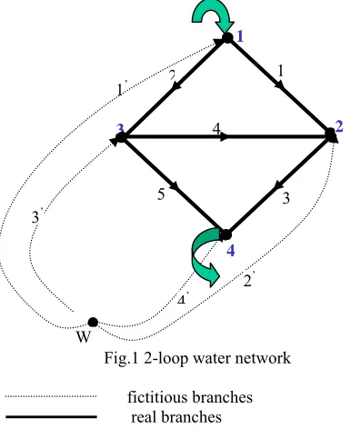
of small example shown in Fig .1, with topology defined by the following incidence matrix:

L=



































1

0

1

0

0

1

1

0

1

0

0

1

1

0

1

0

0

0

1

1

(1)

where rows correspond to the network’s nodes while columns correspond to the branches.

Simulation of Water Networks

Remodeling-Linear-case

Nagib G. N. Mohammed, Adel Abdulrahman, Member, IAENG

G

Manuscript received Oct. 06, 2012; revised Feb. 06, 2013.

First A. is with Community Collage Sana’a & University of Science & Technology, Yemen (Phone +967 714253491 email:

[email protected])

[image:2.612.76.269.51.287.2]

Fig.1 2-loop water network

fictitious branches real branches

Defining the following quantities describing the state of the water network:

H – the vector of water head in network’s nodes

 - the vector of pressure head in network’s branches

Q – the vector of water flow in network’s branches R – the vector of hydraulic compliance in network’s

branches (depends on pipes’ cross-sections, length, material, etc.)

R =

l

K

2

,

K- the characteristic of the element, l - the element’s length,

the following equations governing the water distribution can be formulated:

- equilibrium of inlets and outlets for nodes:

L Q = -q (2)

- continuity equation for the network’s branches:

LT H =



(3)

- constitutive relation governing local flow in branches

Q = R



(4)

where q denotes external inlet to the system.

The constitutive relation (4) is non-linear. Nevertheless, let me assume temporarily linearity of this relation. Substituting Eqs. (4) and (3) to (2), the following formula can be obtained:

L R



LT H = q (5)

Describing the water network shown in Fig.1, the above set of equations takes the following form

   

 

   

 

    

 

   

 

   

 

   

 

  



   



 

  

 



0 0 0

0

0 1

4 3 2 1

' 4 5 3 5 3

5 5 4 2 4 2

3 4

4 3 1 1

2 1

2

1 q

H H H H

R R R R R

R R R R R R

R R

R R R R

R R

R R

(6)

where:

)

( 0 4

' 4

4 R H H

q   , R =

l

K

2

,

K- the characteristic of the element, l - the element’s length,

H – denotes the water pressure in the node (height of water)

q – denotes the flow in the branch,

and it was assumed that the network is supplied only through the node No.1 (inlet with intensity q1) and the only

outlet is through the node No.4 (the coefficient

_R

' 4=1). 0

' 3 ' 2

R



R

, what means, that the outlets in nodes No.2 and 3 vanish.

I. III.VDM-BASED SIMULATION OF PARAMETER

MODIFICATION

Analogously to the Virtual Distortion Method (VDM) applicable to the truss structures (cf.[3]) let us postulate that local modification of a network parameter can be introduced into the system through the virtual distortion 0 _,

incorporated into the formula (4):

LR(LT_{H - }0_{) = q (7)}

The virtual distortion i0 is of the same character as the

pressure head i (see Fig. 2) and its physical meaning is an

[image:2.612.345.505.570.698.2]

additional pressure head externally forced in branch “ i “ (e.g. due to a locally installed pump).

Fig. 2 Distortion simulating water flow (pressure head modification) in branch No. 4

1

1 1’

2

2’

3

3’

4’

4 3 4

5

W

2

1

1 2

3

4

3 4

5

The influence of virtual distortions on the resultant flow redistribution can be calculated using the so-called

influence matrix Dij collecting i responses (row-wise) in

terms of water heads

H

@_i 01 induced in the network by imposing the unit virtual distortion



o

j=1 generated

consecutively in each network branch j. Thus each influence vector

H

@_i 01 can be calculated on the basis of the following equation obtained from Eq. (7):

LRI

*

q

H

L

R

L

T @_01





(8)

The vector q* disregards the external inlet and outlet (the flow is now provided by the imposition of virtual distortion), and it accounts for the water flow distribution in the closed network (cf. Eq. (6)). There is a set of j (j the number of branches) equations (8) to be solved in order to create the full influence matrix D. Each time the right hand-side changes as the unit virtual distortion is applied to another branch. In practice this can be realised by applying a pair of inlets-outlets Lik Rkj



0j corresponding to each branch

(cf. Eq. (7)) – it is the so-called compensative charge. So, the parameter modification in the system is accounted for by superposing the so-called linear response of the original network and the so-called residual response due to imposition of the virtual distortion. Therefore, the resultant water head distribution can be expressed as:











j 0 j ij L i R i L i

i

H

H

H

D

H



(9)

and the resultant water flow as:

















j 0 j ij ij T ij j L j R j L j

j

Q

Q

Q

R

L

D

Q





(10)

The analogous set of relations governs the VDM based approach to modifications of truss structure system [3]. Coming back to the example shown in Fig. 2, let us generate the unit virtual distortion in branch No. 4, connecting the nodes Nos. 2 & 3. The corresponding set of equations (8), accounting for boundary conditions (i.e. outlet in node No.4), takes the following form:



















































































































   

0

R

R

0

H

H

H

H

R

R

R

R

R

0

R

R

R

R

R

R

R

R

R

R

R

R

0

R

R

R

R

0 4 4 0 4 4 1 @ 4 1 @ 3 1 @ 2 1 @ 1 ' 4 5 3 5 3 5 5 4 2 4 2 3 4 4 3 1 1 2 1 2 1 0 0 0 0





    (11)

where



0₄



1

. Assuming the following data: K₁=0.2 m3_/s,

K2=K3=K4=K5=0.4 m3/s, l1=l2=l3=l5=10.000 m, l₄=14.142 m,

q1=0.050 m3/s, H0=0.000 m, we get the following set of

equations for the water head distribution:

                                                      0 011 . 0 011 . 0 0 H H H H 032 . 1 016 . 0 016 . 0 0 016 . 0 043 . 0 011 . 0 016 . 0 016 . 0 011 . 0 031 . 0 004 . 0 0 016 . 0 004 . 0 02 . 0 1 @ 4 1 @ 3 1 @ 2 1 @ 1 0 0 0 0     (11a)

The resulting distribution of water heads

H

@01_{= [0.151,} -0.251, 0.251, 0.000]T _{constitutes the 4th column of the}

influence matrix D. Continuing this procedure for virtual distortions generated in other branches, the full influence matrix can be determined as:

Taking into account relation (3) and applying it consecutively to each influence vector

H

@01, another influence matrix Dε _{can be created, collecting the response} to unit virtual distortions in terms of the pressure head

1 0 @ 



.





















































678

.

0

251

.

0

322

.

0

071

.

0

071

.

0

355

.

0

503

.

0

355

.

0

142

.

0

142

.

0

322

.

0

251

.

0

678

.

0

071

.

0

071

.

0

071

.

0

101

.

0

071

.

0

828

.

0

172

.

0

284

.

0

402

.

0

284

.

0

686

.

0

314

.

0

D

(12)

VI. SIMULATION OF NETWORK REMODELLING (ELEMINATION OF BRANCH

First, let us demonstrate how virtual distortion generated a chosen branch (e.g. in the branch No.4) can simulate the network modification due to total blocking flow in this branch. To this end, the condition of flow vanishing in the branch under remodelling (Q4 = 0) should be postulated,

where resultant state of flow redistribution is calculated from the formulas superposing linear response of the original network configuration and the component induced by unknown virtual distortion:











  0 0

)

(

ij ij j j i L i i j ij j L i i

D

R

Q

Q

D















(13)

Therefore, the virtual distortion to be generated in branch No.4 to simulate complete blocking of local flow can be calculated from the following condition:

Q

4



Q

4



R

i

(

D

44



1

)



40



0

L

or making use of (4)



4L



D

ij



04





04

what leads to:

1

,

34

1

44 4 0 4









D

L 



Finally the pressure head as well as the flow in modified network is (after substitution value (14) to relations (6)) as the following:

m

D

L 0

₃

_,

₀₄

_,

₃₉₆

_*

₁

_,

₃₄

₃

_,

₅₇

4 14 1

1



















m

D

L 0

₂

_,

₃₆₅

_,

₀₉₉

_*

₁

_,

₃₄

₂

_,

₂₃

4 24 2

2



















m

D

L 0

₁

_,

₂₂₅

₀

_,

₂₄₇

_*

₁

_,

₃₄

₀

_,

₈₉

4 34 3

3



















m

D

L 0

₁

_,

₉

₀

_,

₂₄₈

_*

₁

_,

₃₄

₂

_,

₂₃

4 54 5

5



















and the flows:











0

0

,

01216

0

,

004

*

0

,

396

*

1

,

34

4 14 1 1

1

Q

R

D





Q

L

0,0143 m3_/s













0

0

,

03784

0

,

016

(

0

,

099

)

1

,

34

4 24 2 2

2

Q

R

D





Q

L

0,0357 m3_/s













0

0

.

0196

0

.

016

(

0

.

247

)

1

.

34

4 34 3 3

3

Q

R

D





Q

L

0,0143 m3_/s















0

0

.

0304

0

.

016

0

.

248

1

.

34

4 54 5 5

5

Q

R

D





Q

L

0,0357 m3_/s

For comparison, let us solve the set of equations (13) taking into consideration excluding the element No. 4 (i.e. assuming R4 = 0 and disregarding column 4 in the matrix L)

one can get the following set of equations:



























































































00

.

0

00

.

0

00

.

0

05

,

0

032

.

1

016

.

0

016

.

0

000

.

0

016

.

0

032

.

0

000

.

0

016

.

0

016

.

0

000

.

0

02

.

0

004

.

0

000

.

0

016

.

0

004

.

0

020

.

0

' 4 ' 3 ' 2 ' 1

H

H

H

H

The resulting distribution of water head is: H’ ₌

[4.514 0.943 2.282 0.05]T_{, which leads to the following}

state of pressure head as well as the flow in modified network (after substitution H’ to (3) and (13)):

m

57

,

3

943

,

0

514

,

4

H

H

ε

1



1'



'2







m

23

,

2

282

,

2

514

,

4

H

H

ε

' 3 ' 1

2











m

89

,

0

05

,

0

943

,

0

H

H

ε

' 4 ' 2

3











m

23

,

2

05

,

0

282

,

2

H

H

ε

5



'3



'4







and the flows:















0

0

,

01216

0

,

004

0

,

396

1

,

34

4 14 1 1

1

Q

R

D





Q

L

0,0143 m3_/s

0357

,

0

34

,

1

)

099

,

0

(

016

,

0

03784

,

0

0 4 24 2 2

2



Q



R

D













Q

L ε

m3_/s

0143

,

0

34

,

1

)

247

,

0

(

016

,

0

0196

,

0

0 4 34 3 3

3



Q



R

D















Q

L ε

m3_/s

0357

,

0

34

,

1

248

,

0

016

,

0

0304

,

0

0 4 54 5 5

5



Q



R

D













Q

L ε

m3_/s

States (3) as well as (4) are the same, what demonstrates that virtual distortion (14) models properly the assumed modification.

Multiplying the network response HR = [0.151 0.251

-0.251 0.000] for the unit virtual distortion

_

0

4 = 1 7 by the

determined above value,



04 the searched correction to

pressure distribution in the original network can be calculated (Fig.3c) and the resultant pressure distribution for the modified network: H = HL + 1.34 HR can be also

determined (Fig.3b). Similarly, other, various types of the network modifications can be simulated through virtual distortions using determined once the initial system matrix, the linear response HL and the influence matrix D.

Fig.3 Pressure distributions for the original (a), locally distorted (b) and modified (c) networks

For large water networks with small, local modifications the above VDM based approach is much cheaper numerically than the classical way through recomposing and solving the modified system.

In the case of nonlinear problem formulation a superposition of two virtual distortion fields has to be taken into consideration. The first one, 0 _{modeling system redesign}

and the second, 0 _{modeling physical nonlinearity of the}

system (cf. § 3).

V. CONCLUSION

The main advantages of the VDM based approach to the water network analysis WATNET-M are the reduction of numerical costs and avoidance of iteration due to incremental approach in the analysis of water network. The numerical cost of linear analysis consists (in WATNET-M) of:

- Solving the linear problem (7).

REFERENCES

[1] Biedugnis S., Smolarkiewicz M. Model matematyczny sieci wodociągowej na potrzeby projektowania i analizy jej działania, praca doktorska, Warszawa, 2001.

[2] Cross H. (1936) Analysis of Flow in Networks of Conduits or Conductors, University of Illinois Engineering Experiment Station Bulletin, No. 286 [3] Holnicki-Szulc J., Gierlinski J.T. (1995) Structural

Analysis, Design and Control by the Virtual Distortion Method, J. Wiley & Sons, Chichester, U.K.

[4] Kolakowski P., Holnicki-Szulc J. (1998) Sensitivity Analysis of Truss Structures (Virtual Distortion Method Approach), International Journal for Numerical Methods in Engineering, 43, pp. 1085-1108

[5] Cesario, A. L. (1995). Modeling, Analysis, and Design of Water Distribution Systems. American Water Works Association, Denver, Colorado.

[6] Seidler, M. (1982). "Obtaining an Analytical Grasp of Water Distribution Systems." Journal of the American Water Works Association, 74(12).

[7] Loubser, B. F., and Gessler, J. (1994). "Computer Aided Optimization of Water Distribution Networks." Proceedings of the AWWA Annual Conference, American Water Works Association, New York, New York.

[8] Mays, L. W., ed. (2000). Water Distribution Systems Handbook. McGraw-Hill, New York, New York. [9] C. Biscos, M Mulholland, M-V Le Lann, CA Buckley,

and CJ Brouckaert, “ Optimal operation of water distribution networks by predictive control using MINLP” water S. A., Vol. 29, No. 4, PP. 393 – 404, 2003