Cattle feedlot dust – laser diffraction analysis of size distribution and estimation of emissions from unpaved roads and wind erosion

(1)

CATTLE FEEDLOT DUST – LASER DIFFRACTION ANALYSIS OF SIZE DISTRIBUTION AND ESTIMATION OF EMISSIONS FROM UNPAVED ROADS AND WIND EROSION

by

HOWELL B. GONZALES

B.S., University of the Philippines, Los Baños Laguna, Philippines 2001

A THESIS

submitted in partial fulfillment of the requirements for the degree MASTER OF SCIENCE

Department of Biological and Agricultural Engineering College of Engineering

KANSAS STATE UNIVERSITY Manhattan, Kansas

2010

Approved by: Major Professor Ronaldo G. Maghirang

(2)

Copyright

HOWELL B. GONZALES

(3)

Abstract

Large cattle feedlots emit considerable amounts of particulate matter (PM), including TSP (total suspended particulates), PM10 (PM with equivalent aerodynamic diameter of 10 µm or

less), and PM2.5 (PM with equivalent aerodynamic diameter of 2.5 µm or less). Particulate

emissions result from pen surface disturbance by cattle hoof action, vehicle traffic on unpaved roads and alleyways, and wind erosion. Research is needed to determine concentrations of various size fractions, size distribution, and emission rates from various sources in feedlots. This research was conducted to measure particle size distribution using laser diffraction method and estimate emissions from unpaved roads and wind erosion.

Particle size distribution and concentrations of PM10 and PM2.5 at a commercial cattle

feedlot in Kansas (Feedlot 1) were measured over a 2-yr period. The feedlot had a capacity of 30,000 head and total pen area of 50 ha and was equipped with a sprinkler system for dust control. Collocated low-volume samplers for TSP, PM10, and PM2.5 were used to measure

concentrations of TSP, PM10, and PM2.5 at the upwind and downwind edges of the feedlot. Dust

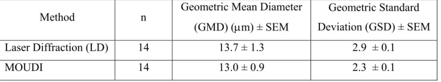
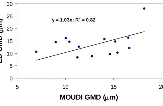
samples that were collected by TSP samplers were analyzed with a laser diffraction analyzer to determine particle size distribution. Particle size distribution at the downwind edge of the feedlot was also measured with micro-orifice uniform deposit impactor (MOUDI). The laser diffraction method and MOUDI did not differ significantly in mean geometric mean diameter (13.7 vs. 13.0 μm) but differed in mean geometric standard deviation (2.9 vs. 2.3). From laser diffraction and TSP data, PM10 and PM2.5 concentrations were also calculated and were not

significantly different from those measured by low-volume PM10 and PM2.5 samplers (122 vs.

131 μg/m3_{for PM}

10; 26 vs. 35 μg/m3 for PM2.5). Both PM10 and PM2.5 fractions decreased as

pen surface moisture contents increased, while the PM2.5/PM10 ratio did not change much with

pen surface moisture content.

Published emission models were used to estimate PM10 emissions from unpaved roads

and wind erosion at Feedlot 1 and another nearby feedlot (Feedlot 2). Feedlot 2 had a capacity of 30,000 head, total pen surface area of 59 ha, and used water trucks for dust control. Estimated PM10 emissions from unpaved roads and wind erosion were less than 20% of total PM10

(4)

emissions obtained from inverse dispersion modeling. Further research is needed to establish the applicability of published emission estimation models for cattle feedlots.

(5)

List of Figures

Figure 2.1 Four distinct layers of the pen surface (adapted from: ACFA, 2002) ... 6

Figure 2.2 Microorifice Uniform Deposit Impactor (MOUDI): (a) schematic diagram; (b) photograph ... 11

Figure 2.3 Interactions between particle and light beam (adapted from: Merkus, 2008)... 13

Figure 2.4 Soil erosion by wind (source: http://www.weru.ksu.edu/weps/wepshome.html) ... 20

Figure 3.1 Feedlot 1 equipped with a water sprinkler system ... 37

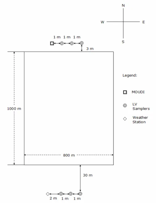
Figure 3.2 Schematic diagram of the feedlot showing relative locations of samplers and weather station (not drawn to scale). ... 39

Figure 3.3 Beckman Coulter LS 13 320 Operation ... 41

Figure 3.4 Comparison of the MOUDI and LD in geometric mean diameters (GMDs)... 45

Figure 3.5 Comparison of MOUDI and LD in geometric standard deviations (GSDs) ... 46

Figure 3.6 Effect of wind speed on geometric mean diameter (GMD) obtained from LD method ... 49

Figure 3.7 Mean volume percent at different aerodynamic diameters ... 51

Figure 3.8 Particle size distribution comparison between events with water application and events without water application... 52

Figure 3.9 Effects of pen surface moisture content on PM concentrations measured using the LD method: (a) PM10 and (b) PM2.5. ... 53

Figure 3.10 Pen surface moisture content dependence of PM fractions measured using the LD method: (a) PM10 fraction and (b) PM2.5 fraction. ... 53

Figure 3.11 Effect of pen surface moisture content on PM2.5/PM10 ratio measured using the LD method... 54

Figure 3.12 Effect of pen surface moisture content on mean geometric mean diameter measured using the LD method... 55

Figure 4.1 Monthly PM10 emissions (metric tons) using the US EPA AP-42 model. Error bars represent standard deviation of the PM10 measurements from the mean PM10 emissions. .. 70

Figure 4.2 Feedlot 1 net PM10 flux vs. wind speed using TEOM data ... 71

(9)

Figure 4.4 Monthly PM10 emissions (metric tons) using the SWEEP model. Error bars represent

standard deviation of PM10 measurements from the mean PM10 emissions... 73

Figure 4.5 Monthly mean wind speed from 2008 – 2009. Error bars represent standard deviation of wind speeds from the mean monthly wind speed... 74 Figure C.1 SWEEP "Field Tab" Interface ... 89 Figure C.2 Daily output information showing the scroll down option to choose between

calculated friction velocities and threshold friction velocity... 90 Figure C.3 Sample output from SWEEP showing soil loss parameters ... 91

(10)

List of Tables

Table 2.1 Typical Nonpoint Source Categories (US EPA, 2004)... 5 Table 2.2 National Ambient Air Quality Standards for Particulate Matter ... 7 Table 2.3 Control efficiency guide (Countess Environmental, 2006) ... 17 Table 3.1 Comparison of laser diffraction and cascade impactor in geometric mean diameter and geometric standard deviation ... 44 Table 3.2 Comparison of cumulative fraction and particle fraction methods in determining PM

fractions and concentrations... 47 Table 3.3 Downwind 24-h mass concentrations (μg/m3_{) - laser diffraction vs. low-volume}

samplers ... 47 Table 3.4 Upwind 24-h mass concentrations (μg/m3_{) - laser diffraction vs. low-volume samplers}

... 48 Table 3.5 Effect of sampling period (day vs night) on geometric mean diameter (from LD

method) ... 49 Table 3.6 Comparison of mean geometric mean diameter and mean geometric standard

deviation between the warm and cold months ... 51 Table 3.7 Effects of water application on geometric mean diameter and geometric standard

deviation... 52 Table 4.1 Mean percent surface material components for the two feedlots ... 67 Table 4.2 Annual emission rates (metric tons/year) from the two feedlots using US EPA AP-42

wind erosion on a dry exposed surface ... 68 Table 4.3 Comparison of wind erosion parameters determined using US EPA AP-42 between

2008 and 2009... 69 Table 4.4 Estimated PM10 emission rates using the SWEEP model... 74

Table 4.5 Summary of the meteorological conditions ... 75 Table 4.6 Comparison of wind erosion parameters for the SWEEP model between 2008 and

2009... 75 Table 4.7 Comparison of emission factors (kg/1000hd-day) for the two-year span ... 77 Table A.1 Cattle on feed 1000+ capacity feedlots (USDA NASS, [2009, 2005, 2000]) ... 82

(11)

Table B.1 Sample data from laser diffraction analysis ... 83 Table B.2 Geometric mean diameter (GMD) and geometric standard deviation (GSD) values for

comparing LD and MOUDI... 86 Table B.3 Geometric mean diameter (GMD) and geometric standard deviation (GSD) values for

Feedlot 1 (downwind) during warm months (April to October)... 87 Table B.4 Geometric mean diameter (GMD) and geometric standard deviation (GSD) values for

(12)

List of Acronyms

ACFA Alberta Cattle Feeders’ Association

AERMOD American Meteorological Society/Environmental Protection Agency Regulatory Model

AP-42 US EPA Compilation of Air Pollutant Emission Factors

ARD Air Resources Division

CAA Clean Air Act

CAFO Concentrated Animal Feeding Operation CARB California Air Resources Board

da Equivalent aerodynamic diameter (µm)

dp Particle diameter (µm)

EF Emission Factor (kg/1000 hd-day)

EU European Union

FAO Food and Agriculture Organization

FEM Federal Equivalent Method

FRM Federal Reference Method

GMD Geometric Mean Diameter

GSD Geometric Standard Deviation

ISO International Organization for Standardization

LD Laser Diffraction

LV Low-Volume

MC Pen surface moisture content (%)

mj Mass fraction of particles in the jth size range (dimensionless) MMD Mass Median Diameter (µm)

MOUDI Micro-Orifice Uniform Deposit Impactor MRI Midwest Research Institute

MsLI Multi-stage Liquid Impinger NAAQS National Ambient Air Quality Standards NASS National Agricultural Statistics Service

NGI New Generation Impactor

NRC National Research Council

NRCS National Resources Conservation Service NSPS New Source Performance Standards PF2.5 PM2.5 fraction

PF10 PM10 fraction

Pi Erosion potential (g/m2)

PM Particulate matter

PM2.5 Particulate matter with equivalent aerodynamic diameter of 2.5 µm or less

PM10 Particulate matter with equivalent aerodynamic diameter of 10 µm or less

PSD Particle Size Distribution

PTFE Polytetrafluoroethylene

RAAS Reference Ambient Air Sampler Re Reynolds number (dimensionless)

s Surface silt content (%)

(13)

SWEEP Single-event Wind Erosion Evaluation Program TEOM TM Tapered-Element Oscillating Microbalance TSP Total suspended particulates

u Wind speed (m/s)

ut Threshold wind speed (m/s)

u* Friction velocity (m/s) u*t Threshold friction velocity (m/s)

USDA United States Department of Agriculture

US EPA United States Environmental Protection Agency

USDA ARS United States Department of Agriculture Agricultural Research Service USDA SCS United States Department of Agriculture Soil Conservation Service VMT Vehicle miles traveled (miles/year)

VOCs Volatile Organic Compounds

W Mean vehicle weight (tons)

W*e Wind erosive energy (m3/s3)

WEPS Wind Erosion Prediction System WRAP Western Regional Air Partnership

z Height (m)

(14)

List of Symbols

χ Shape factor (dimensionless)

κ von Karman constant (0.4)

ρa Air density (g/cm3)

(15)

Acknowledgements

I would like to acknowledge our dear Lord Jesus Christ who gave me wisdom and knowledge to get through with my MS studies here at Kansas State University and had kept me strong through the tumultuous times especially during the loss of my mom which occurred two weeks before I got here in the United States. You are an amazing God indeed and worthy of all praises!

Secondly, I would like to thank my wife, Gilda, for the amazing support, though there were rough times, you are indeed my inspiration on continuing my education and hopefully we can continue to be a blessing to others. To my family, my Dad who is equally supportive of me from the start of my studies here, I thank you for the love and confidence you have put in me. My sister Hazel who was all the more present and active in prayers when I was starting up to the end of my MS studies; the same with my sister Haidee who gave me an opportunity to study here and vouching for me as her little brother who wanted to pursue an advanced degree; my brother Harvey and Ate Mai and my nephews Liam and Lance who equally gave inspiration and joy especially when I talk with them online in between the stressful hours of writing the manuscript.

I would like to thank my adviser, Dr. Ronaldo Maghirang, for opening an opportunity for me to pursue graduate studies here at Kansas State University. Thank you for the knowledge that you have imparted to me from the very beginning of my MS schooling. Thank you for all the advice and thank you for your patience, support and encouragement especially throughout the writing of my manuscript.

I would like to thank both of my committee members, Dr. Jeff Wilson and Dr. Joseph Harner for their inputs and openness to inquiries regarding the writing of the manuscript. Thank you Dr. Wilson for welcoming me at USDA with open arms when I was just starting to know more about the LD instrument.

The support provided by USDA NIFA Special Research Grant, “Air Quality: Reducing Air Emissions from Cattle Feedlots and Dairies (TX and KS)” through Texas AgriLife Research and Extension Center; USDA NIFA Grant No. 2007-35112-17853, "Impact of water sprinkler systems on air quality in cattle feedlots;" and K-State Research and Extension is acknowledged. Cooperation of KLA Environmental Services and feedlot managers/operators is also greatly appreciated and acknowledged.

(16)

I also would like to thank the USDA WERU team, Dr. Tatarko, Dr Wagner and Dr. Hagen who helped me a lot in running the SWEEP model. Dr. Hagen, I am thankful to you so much for your vast inputs in my wind erosion discussion.

I would like to thank the BAE Air Quality Team for welcoming me with open arms and taught me nuances of the tasks and responsibilities of being part of the group. Thank you for all the knowledge Ate Edna, you are a big sister to me and a “boss” at the same time; your inputs and advice taught me so much. And to Henry, a brother to me who helped me a lot with my program simulation input and thank you for the help academically when I was starting as a graduate student at K-State. To Li, my “senior”, who amazes me all the time and a very good friend and mentor to me when I was just starting my courses. To my buddy Curtis, yo! man! I will never forget the certificate of appreciation I got from you when I won the Final Four Tournament prediction. Haha!

To the Filipino community who have embraced Gilda and I as part of the group; all of you who were hospitable and caring to us especially Tita Beth when we first transferred to Jardine. Thank you for providing the “best” dining table to us; don’t worry Tita Beth, it is well taken cared of! To Ate Peewee who was a big sister and mentor to me when I was doing the LD analysis, thank you for the knowledge you shared to me. To Kuya Eric, a big brother and a friend who accommodated me when I was starting my K-State life, you are indeed a blessing to me. To the Moog family who were equally hospitable when I was just starting to know more about Manhattan, KS, I am very blessed to have you as part of my life.

To the Living Word Church family, our pastors, the music ministry, the jail ministry, you are all indeed great spiritual blessings to us! Thank you for all the prayers and support that you have given us, your prayers are more than enough! To Grandpa Rex, Grandpa Marion, Grandma Sharry, Grandma Azer and Grandma Nancy, you are all amazing brothers and sisters in Christ! Thank you for the prayers and support all of you have given us that truly opened the windows of spiritual blessings not only to us, but to others whom we were able to inspire through the

message of our Lord Jesus Christ. To Lesa and Barry Patterson, without you, we won’t be having such a reliable and an almost brand new means of transportation. It really helped me a lot going to school, church, and back home especially when our old car almost died which was the time when the weather started to get cold. A really perfect blessing from God your whole family is to us! Thank you all so much!

(17)

Dedication

I would like to dedicate this manuscript to my loving, caring and very supportive late mother, Purita Gonzales, who died of cancer two weeks before I got to start my graduate studies here in the United States. I know you were happy that I got accepted for studies in the United States. I am so blessed to have a mother like you, yes we the 4-H Kids are so blessed to have a mom like you. I know that you were not able to have a glimpse of this fruit of labor of mine and also attend my graduation but I was more than inspired to dedicate this treasure to you. Though you were already gone when I started my graduate studies, mommy, I miss you, the whole Gonzales family misses you, and we all love you!

(18)

CHAPTER 1 - Introduction

1.1 Background

There is increasing concern on air pollutant emissions from cattle feeding operations because of their increasing sizes and geographic concentrations (National Research Council, 2003). These operations generally involve feeding cattle in confined, open areas, with stocking densities of about 14 m2/hd or greater. Each cattle produces about 900 kg of dry manure during its stay in the feedlot (Sweeten et al., 1998). Warm temperatures, low humidity, and high wind speed promote rapid evaporation of water from the manure making it loose and more susceptible to suspension due to cattle hoof action and wind scouring (Amosson et al., 2006).

Emitted PM is a concern because of potential adverse health and environmental effects (Cole et al., 2008). PM, especially PM2.5 (PM with equivalent aerodynamic diameter of less than

or equal to 2.5 µm), is readily inhaled and can be deposited in lung tissue, resulting in respiratory ailments (Saxton et al., 1999). Six criteria air pollutants, including PM, and 187 air toxics are regulated by the US Clean Air Act (CAA) (US EPA, 1987) because of their risks to human health and environment. National Ambient Air Quality Standards (NAAQS) were created for the criteria pollutants to help control emissions that pose great risk to human health and environment (US EPA, 1987). Agricultural sources, including cattle feedlots, have not been included in the implementation of NAAQS. Recently, however, US EPA has amended the rule for inclusion of agricultural operations (US EPA, 2004). Also, limited information is available on emission rates from animal feeding operations (US EPA, 1995).

Measuring and characterizing PM is necessary for effective implementation of air quality standards and development of abatement measures. Two important PM characteristics are concentration and size distribution. Measurements of PM concentrations in cattle feedlots have used federal reference method (FRM) samplers (Sweeten et al., 1988; Purdy et al., 2007) and federal equivalent method (FEM) samplers (Bonifacio, 2009; McGinn et al., 2010).

Measurements have considered total suspended particulates (TSP), PM10 (PM with equivalent

aerodynamic diameter of 10 µm or less), and PM2.5 (PM with equivalent aerodynamic diameter

of 2.5 µm or less). Purdy et al. (2007) used high volume reference samplers for PM10 and PM2.5

(19)

microbalance (TEOMTM) PM10 monitors to measure PM10 concentrations upwind and downwind

of two large cattle feedlots in Kansas. Guo et al. (2009) used FRM high-volume, FEM TEOMTM, and low-volume PM10 samplers in cattle feedlots in Kansas. McGinn et al. (2010)

measured PM10 concentrations in cattle feedlots in Australia using FEM beta attenuation mass

monitors.

Various techniques have been used to measure particle size distributions (PSDs) in cattle feedlots. Coulter Counters (e.g., Wanjura et al., 2004; Purdy et al., 2007) and cascade impactors (Guo et al., 2011) have been used in several studies. In related areas, laser diffraction has been used. For example, Cao (2009) evaluated particle size distribution in a layer operation through several instruments, including laser scattering particle size analyzer, laser diffraction analyzers, and Coulter Counter.

Laser diffraction has potential to enhance measurement of size distribution and

concentrations of various size fractions in animal feeding operations, including cattle feedlots. This method is easier to use and presents a wider size range compared to conventional impactors. This wider size range will be helpful in evaluating concentrations and size distributions of

particles more effectively.

Limited studies have been conducted to establish contributions of unpaved roads on cattle feedlot PM emissions and none had reported emissions brought about by wind erosion in cattle feedlots. Wanjura et al. (2004) reported about 80% of total emissions from cattle feedlots are brought about by unpaved roads, while Hamm (2005) reported 53% contribution of unpaved roads toward total emissions. The San Joaquin Valley Air Pollution Control District (SJV APCD) reported an emission factor of 0.72 kg/hd-yr for unpaved roads from a cattle feedlot in San Joaquin Valley, CA. (Countess Environmental, 2006). With limited data, studies on

estimating such contributions are necessary to establish better understanding of their mechanisms and develop control methods.

1.2 Objectives

This study was conducted to:

(1) Determine applicability of laser diffraction in measuring size distribution of particles emitted from cattle feedlots; and

(20)

(2) Estimate contributions of unpaved roads and wind erosion to total PM emission from cattle feedlots.

Results of the first objective can be useful in deciding whether or not to use laser diffraction as alternative for measuring PSD and PM concentration in open cattle feedlots. The second objective can be useful in estimating which of the miscellaneous sources are major contributors to PM emissions aside from cattle hoof action on pen surfaces.

1.3 References

Amosson, S.H., B. Guerrero, and L.K. Almas. 2006. Economic analysis of solid-set sprinklers to control dust in feedlots. Journal of Agricultural & Applied Economics 38.2 (August 2006): 456.

Bonifacio, H. F. 2009. Particulate matter emissions from commercial beef cattle feedlots in Kansas. MS Thesis. Manhattan, Kan.: Kansas State University.

Cao, Z. 2009. Determination of particle size distribution of particulate matter emitted from a layer operation in Southeastern U.S. MS Thesis. Raleigh, N.C.: North Carolina State University. Cole, N.A., R. Todd, B. Auvermann, and D. Parker. 2008. Auditing and assessing air quality in

concentrated feeding operations. The Professional Animal Scientist 24: 1-22. Countess Environmental. 2006. WRAP fugitive dust handbook. Prepared for Western

Governor’s Association, Denver, Colo. Available at

http://www.wrapair.org/forums/dejf/fdh/content/FDHandbook_Rev_06.pdf. Accessed 21 March 2010.

Guo, L., R. G. Maghirang, E. B. Razote, J. Tallada, J. P. Harner, and W. Hargrove. 2009. Field comparison of PM10 samplers. Applied Engineering in Agriculture 25(5): 737-744.

Guo, L., R. G. Maghirang, E. B. Razote, S. L. Trabue, and L. McConnell. 2011. Concentration of particulate matter in large cattle feedlots in Kansas. For: Journal of Air & Waste

Management (In review).

Hamm, L.B. 2005. Engineering analysis of fugitive particulate matter emissions from cattle feedyards. MS thesis. College Station, Tex.: Texas A&M University.

McGinn, S.M., T.K. Flesch, D. Chen, B. Crenna, O.T. Denmead, T. Naylor, and D. Rowell. 2010. Coarse particulate matter emissions from cattle feedlots in Australia. Journal of Environmental Quality 39(3): 791-798.

(21)

National Research Council (NRC). 2003. Air emissions from animal feeding operations: Current knowledge, future needs. Washington, D.C.: National Academies Press. Purdy, C.W., R.N. Clark, and D.C. Straus. 2007. Analysis of aerosolized particulates of

feedyards located in the Southern High Plains of Texas. Aerosol Science and Technology 41(5): 497–509.

Saxton, K., D. Chandler, and W. Schillinger. 1999. Wind erosion and air quality research in the Northwest U.S. Columbia Plateau: Organization and progress. In E.E. Stott, R.H.

Mohtar, and G.C. Steinhardt (eds). Sustaining the Global Farm – Selected papers from the 10th International Soil Conservation Organization Meeting, 24-29 May, West Lafayette, Ind.

Sweeten, J.M., C.B. Parnell, R.S. Etheredge, and D. Osborne. 1988. Dust emissions in cattle feedlots. Veterinary Clinics of North America, Food Animal Practice 4(3): 557-578. Sweeten, J.M., C.B. Parnell, B.W. Shaw, and B.W. Auvermann. 1998. Particle size distribution

of cattle feedlot dust emission. Transactions of the ASAE 41(5): 1477-1481. U.S. Environmental Protection Agency (US EPA). 1987. National ambient air quality

standards. 40 CFR Part 70. Research Triangle Park, NC: US EPA. Available at http://www.epa.gov/air/caa. Accessed 10 July 2010.

U.S. Environmental Protection Agency (US EPA). 1995. AP-42: Chapter 9 Food and agricultural industries. Research Triangle Park, NC: US EPA. Available at http://www.epa.gov/ttn/chief/ap42/ch09/index.html. Accessed 10 July 2010.

U.S. Environmental Protection Agency (US EPA). 2004. Use of a performance based approach to determine data quality needs for the PM-coarse (PMc) standard. Research Triangle Park, NC: US EPA. Available at http://www.epa.gov/airnow/particle/pm-color.pdf. Accessed 10 July 2010.

Wanjura, J.D., C.B. Parnell, B.W. Shaw, and R.E. Lacey. 2004. A protocol for determining a fugitive dust emission factor from a ground level area source. ASAE/CSAE Paper No. 044018. St. Joseph, Mich.: ASAE.

(22)

CHAPTER 2 - Literature Review

2.1 Particulate Emissions from Cattle Feedlots

2.1.1 Background

In the U.S., there has been a steady increase in the number of beef cattle slaughtered from 2004 to 2008, with a slight decrease in 2009 (USDA, 2009). The number of cattle feedlots, however, has generally decreased, indicating greater stocking densities (USDA, 2009, 2005, 2000). A mixture of PM and gases emanate from these feedlots (Bunton et al., 2007), raising concerns on the health of nearby residents.

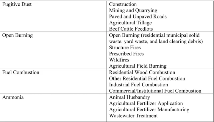
Beef cattle feedlots are considered non-point or open sources because emissions do not originate from a specific source like a chimney, stack or vent (ARD-42, 2010). Airborne particles that originate from cattle feedlots and other non-point sources (Table 2.1) are called fugitive dust emissions (Ferguson et al., 1999).

Table 2.1 Typical Nonpoint Source Categories (US EPA, 2004)

Fugitive Dust Construction

Mining and Quarrying Paved and Unpaved Roads Agricultural Tillage Beef Cattle Feedlots

Open Burning Open Burning (residential municipal solid

waste, yard waste, and land clearing debris) Structure Fires

Prescribed Fires Wildfires

Agricultural Field Burning

Fuel Combustion Residential Wood Combustion

Other Residential Fuel Combustion Industrial Fuel Combustion

Commercial/Institutional Fuel Combustion

Ammonia Animal Husbandry

Agricultural Fertilizer Application Agricultural Fertilizer Manufacturing Wastewater Treatment

(23)

2.1.2 Sources of Particulate Matter in Cattle Feedlots

PM emissions in cattle feedlots come from various sources: cattle activity inside pens, vehicle movement along unpaved roads, feed mills, and wind erosion. The major contributing source for feedlot emissions is cattle hoof action on the dry and loose pen surface, which is a mixture of soil and manure. Figure 2.1 shows a schematic diagram of the pen surface in cattle feedlots (ACFA, 2002). The topmost layer of the pen surface (i.e., manure pack) consists of manure that acts as a sponge as it absorbs water from rain, snow, or urine. It has capacity to hold enough water (up to 25 mm of precipitation) during dry periods, and water readily evaporates from the surface, making it loose. The gleyed or second layer, about 5 to 10 cm thick, is

impermeable because it hinders salt, nutrient, and water penetration to lower layers. This layer is formed by the transformation of organic matter, gel, and slimes aided by poor drainage and lack of oxygen. The third layer is compacted soil/manure layer, about 15 cm thick and made of soil mixed with organic matter from manure. The last layer is natural soil, commonly loam- or clay-based soil (ACFA, 2002).

Figure 2.1 Four distinct layers of the pen surface (adapted from: ACFA, 2002) 2.1.3 PM Regulations in Cattle Feedlots

The NAAQS for PM10 and PM2.5 (Table 2.2, US EPA, 2006a) have been considered

applicable to open cattle feedlots. Emission factors for open cattle feedlots have also been published; for inventory purposes, a PM10 emission factor of 17 tons per 1000 head throughput

(24)

Table 2.2 National Ambient Air Quality Standards for Particulate Matter (Source: http://www.epa.gov/air/criteria.html)

Particle Size Primary Standard (μg/m3₎ _{Averaging Times}

PM10 150 24 h

15 Annual (arithmetic mean)

PM2.5

35 24 h

2.1.4 Measurement of PM and Size Distribution in Feedlots

Limited information is available on concentrations of various size fractions and particle size distribution in cattle feedlots. Most published data have been from cattle feedlots in Texas. Sweeten et al. (1988) investigated three cattle feedlots in Texas and reported net total suspended particulate (TSP) concentration of 412 ± 271 μg/m3_{and median particle diameter of 10.2 ± 1.2}

μm. They also noted that dust concentrations were high during early evening and low during early morning. In a related study, Sweeten et al. (1998) reported mean TSP concentration of 700 ± 484 μg/m3 _{and mean PM}

10 concentration of 285 ± 214 μg/m3 in three cattle feedlots in Texas.

In addition, they observed mass median diameters of particles of 9.5 ± 1.5 μm for TSP samplers and 6.9 ± 0.8 μm for PM10 samplers.

Hamm (2005) reported a range of 113 to 6000 μg/m3_{during a summer sampling period in}

a feedlot in Texas. The feedlot condition was dry with an average temperature of 38 ºC during the day and 21 ºC at night, such that relatively high concentrations of PM were expected.

Purdy et al. (2007) measured PM from four large feedlots in Texas. They reported that three of the four feedlots exceeded the 24-h PM10 NAAQS. Mean PM10 particle sizes for the

feedlots were measured using a laser strategic aerosol monitor. Median PM10 size was 8.3 μm

downwind and upwind of the feedlots.

Razote et al. (2007) investigated a cattle feedlot in western Kansas using tapered element oscillating microbalances (TEOMs) and reported net PM10 concentrations of 115 ± 80 μg/m3 and

mean geometric mean diameter (GMD) of 11.4 ± 2.1 μm. In a related study, Guo et al. (2009) measured PM10 concentrations using high-volume, TEOMs, and low-volume PM10 samplers in

(25)

In two cattle feedlots in Australia, McGinn et al. (2010) reported mean 24-h PM10

concentrations ranging from 9 to 61 μg/m3_{. Feedlot PM}

10 24-h concentrations were close to or

exceeded European Union (EU) and Australian standards twice during the 10-day sampling campaign but did not exceed the US EPA 24-h NAAQS for PM10..

2.1.5 Control of PM Emissions

Feedlot operators and managers have implemented abatement strategies to control dust emissions. The most basic type of abatement is application of water. Razote et al. (2006) indicated decrease in PM10 emission potential of a simulated pen surface from 19.2 mg (control)

to 3.4 mg (at 3.2 mm water) and 2.3 mg (at 6.4 mm water). Bonifacio et al. (2011) reported a control efficiency range of 32-80 % for PM10 of a water sprinkler system in a feedlot.

Pen surface moisture content should be maintained at a level that minimizes both odor and dust emissions. Davis et al. (1997) stated that the pen surface moisture content should be kept at 25 to 35 %. Too much moisture promotes fly and odor problems, while too dry of a pen can lead to significant dust problems.

Another potential abatement strategy is application of materials, including wheat straw and saw dust, on the pen surface. Other control methods include pen cleaning to reduce the amount of loose manure in the pen surface (Rahman et al., 2008). The removed manure is placed in storage or composting area and sometimes covered with soil.

Manipulation of the stocking density, the number of cattle inside the pen, is also a potential dust control measure. Increasing stocking density results in moisture accumulation, causing the pen surface to be compact and less vulnerable to PM emissions (Romanillos and Auvermann, 1999). Razote et al. (2006) mentioned that even without adding water, compacted surface layers could reduce potential emissions (with respect to vertical hoof action) by 30 %. For low and medium moisture contents (20-30 %), soil surface compaction is achieved through cattle trampling (Mullholland and Fullen, 1991; Scholefield and Hall, 1985).

Emissions can also be reduced by feeding cattle during late afternoon or early evening – periods of increased cattle activity (Sweeten et al., 1988). Wilson et al. (2002) found significant reductions in dust concentrations in cattle feedlots by altering feeding strategies. In their study, cattle in control pens were fed normal daily rations (33 %, 33 % and 34 % of total feed rations at 7:10 AM, 10:00 AM, and 12:00 PM, respectively) while cattle in another set of pens were fed

(26)

30%, 20 %, and 50 % at 7:00 AM, 10:00 AM, and 6:30 PM, respectively. Mean PM

concentrations were 177 ± 2 μg/m3_{for control pens and 97 ± 16 μg/m}3_{of dust for test pens.}

Use of shelterbelts and windbreaks can also help in managing dust emissions from open cattle feedlots. This method utilizes trees or vegetation to capture particulates downwind and reduce wind speed toward the site, reducing potential for wind erosion (Carter, 2006).

2.2 Particle Size and Size Distribution

2.2.1 Particle Size

Particle size is one of the most important characteristics of particles. Environmental concerns associated with exposure to PM can be narrowed down into particles being inhaled, which are deposited in different areas of the respiratory system based on their size. Health-based particle-size selective sampling (TSI, 2009) classification of particles with respect to median aerodynamic diameter are as follows: 100 μm (inhalable fraction or fraction of particles that enter the respiratory system through the nose or mouth), 10 μm (thoracic fraction or portion of the inhalable fraction that passes through the larynx and penetrate into the trachea and the bronchial region of the lungs), and 4 μm (respirable fraction or portion of the inhalable fraction that enters the alveoli).

In medical research, deposition pattern and bioavailability are defined using particle size of drug materials as it is allowed to penetrate through the respiratory system during inhalation (Pilcer et al., 2008). A size range of about 1 to 5 μm is the optimum range for particles to deposit deep into the pulmonary system. Larger particles are trapped in the oro-pharynx, while submicrometer particles remain suspended in air for exhalation (Bosquillon et al., 2004).

Vincent (2007) summarized the classification of typical aerosols. Combustion sources such as fume dominate fine (diameter between 0.1 and 2.5 μm) and ultrafine particle regions (diameter < 0.1 μm), while soil dust, construction dust, and road dust are predominantly in the coarser region (diameter > 2.5 μm) (Watson et al., 2000; Lin et al., 2005).

Particle characterization usually involves defining its equivalent diameter. For a spherical particle, particle diameter is unique compared to a non-spherical particle, which does not possess a specific diameter. The concept of equivalent diameter has been used to describe sizes of non-spherical particles. This concept involves determining the size of an equivalent

(27)

sphere that embodies the same properties as the particle in question. At times a single equivalent sphere can be used to represent the behavior of a non-spherical particle in a measurement

technique like sieving, sedimentation and microscopy. Some techniques require rigorous computations because the particle behaves differently in various orientations. The laser diffraction method involves measurement of the light scattering of particles, which are usually different from one angle to another. As such, the different scattering patterns are averaged during the analysis.

Another important factor that affects particle behavior is particle density. For

instruments that measure volume percent, it is necessary to know particle density to compute the mass. Particle density is also important in calculating and changing from the equivalent sphere diameter (dp) to its equivalent aerodynamic diameter (da). Another critical parameter is particle

shape. Various descriptive terms can be applied to particle shape, but for ease of analysis, this property is captured by the incorporation of shape factor (χ) into equations for particle size analysis. For spherical particles, χ = 1.

2.2.2 Geometric Mean Diameter and Geometric Standard Deviation A size distribution is a collection of particles characterized by properties, such as aerodynamic diameter, number, mass or volume fraction. A size distribution is considered monodisperse if 90 % of particles are within 5 % of the median size and polydisperse otherwise (Merkus, 2008). In cattle feedlots, particle size distributions are polydisperse.

For a given size distribution, characteristic parameters are geometric mean diameter (GMD) and geometric standard deviation (GSD) (US EPA, 2010). The GMD (μm) gives the central tendency of a particle size distribution and is expressed as follows (Hinds, 1999):

(2.1) ln GMD ln

∑

= j pj j m d m where dpj = geometric mean of the jth size range, μm

mj = mass fraction of particles in the jth size range

The geometric standard deviation (GSD) describes how wide the size distribution is around the GMD and can be calculated as (Hinds, 1999):

(28)

(2.2) GMD ln GSD ln 2 1 2 ⎟ ⎟ ⎟ ⎟ ⎟ ⎟ ⎠ ⎞ ⎜ ⎜ ⎜ ⎜ ⎜ ⎜ ⎝ ⎛ ⎟ ⎟ ⎠ ⎞ ⎜ ⎜ ⎝ ⎛ =

∑

j j p j m d m 2.2.3 Cascade Impactor

Size distribution of airborne particles is typically measured using a cascade impactor. In a cascade impactor, impaction is achieved though a jet of particle-laden air, which is allowed to

make contact with a flat impaction plate (Figure 2.2). Particles are separated by having large particles retained on the plate, while smaller particles are delivered with the airflow out of the impaction region, left uncollected. Particles collected on an impaction plate are of specific aerodynamic diameter (Heyder et al., 1986; Marple et al., 1991). The particle size distribution is determined based on the obtained mass fractions of specific size ranges.

Figure 2.2 Microorifice Uniform Deposit Impactor (MOUDI): (a) schematic diagram; (b) photograph

Various types of cascade impactors are available commercially. This study used the microorifice uniform deposit impactor (MOUDI model 100-R, MSP Corp., 2006), which has

(29)

been used in various research. Kleeman et al. (1999) used the MOUDI in evaluating the particle size distribution of emissions from wood burning, meat charbroiling, and cigarette smoking. Wood smoke and meat charbroiling had dominant particles in the range of about 0.1 to 0.2 μm, while particles in cigarette smoke was in the range of 0.3 to 0.4 μm. Kleeman et al. (2000) reported that the smoke from gasoline-powered, light-duty vehicles and light-duty diesel trucks did not differ with particle sizes ranging from 0.1 to 0.2 μm. In a city with dense traffic, Martuzevicius et al. (2004) reported a significant amount of PM2.5 was contributed by particles

with d50 = 0.32 to 1.0 μm. Fang et al. (2005) evaluated the particle size distribution of

atmospheric aerosols at a traffic site during the winter period using MOUDI and nano-MOUDI. The average mass median diameter (MMD) of particles was 0.99 μm. The PM10 represented

94.4 % of TSP, while PM2.5 was 68.9 % of TSP.

Airborne bacteria and endotoxins were measured with the MOUDI (Kujundzic et al., 2006). An environmentally controlled chamber was used to simulate conditions in a home during winter and summer seasons. Airborne bacteria were in the size range of 0.32 to 3.2 μm, while endotoxin ranged in size from 0.056 to 3.2 μm.

In cotton production, Miller et al. (2006) measured the size distribution of dust generated from field preparation during harvesting of cotton seed using a MOUDI. They reported that PM10 represented 96 % (disking) and 83 % (harvesting) of the total mass measured by the

cascade impactor for disking and harvesting, respectively. In addition, PM2.5 represented 51 %

(disking) and 45 % (harvesting), respectively. Use of a tractor in agricultural field operations was studied by Wang et al. (2009). They reported that 92 % of the TSP collected by the impactor represented PM10 particles.

2.2.4 Laser Diffraction Method 2.2.4.1 Light Scattering Theory

Laser diffraction, in a strict sense, is not a true particle size measurement technique, rather it is a particulate system characterization technique (Xu, 2000). Particle size distribution arises from the “best fit” model for light scattering data with the assumption of having spherical particles (Tinke et al., 2008). Mühlenweg and Hirleman (1998) argued that there is not a unique size and shape related diffraction diameter that comes from a diffraction pattern of non-spherical

(30)

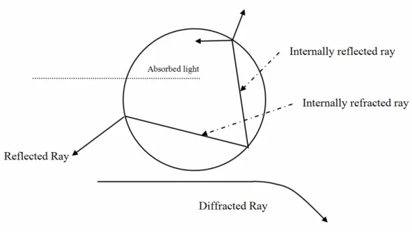
particle. Merkus (2008) stated that laser diffraction is a model-based particle size distribution calculation from an angular pattern of scattered intensities, and the distribution generated is based on the volume of a collection of spherical particles that has identical light scattering patterns as that of the dispersed sample. As the conditioned beam of light strikes the surface of a particle (Figure 2.3), four types of interactions exist between the particle and beam of light (Merkus, 2008):

(a) Fraunhofer diffraction –diffraction of light at the contour of the particle; (b) reflection of light at the particle’s surface, both inside and outside the particle; (c) refraction of light at the interface of particle and dispersion medium; and (d) absorption of light inside the particle.

Figure 2.3 Interactions between particle and light beam (adapted from: Merkus, 2008)

The basic approximation for particle size that was developed as the first optical model was the Fraunhofer theory. Assumptions of the theory include (1) interaction exists only between the light and the particle contour; (2) particles are opaque (i.e., without promoting secondary scattering), circular, and two-dimensional; (3) angle of scattered light is small; (4) wavelength of light is much smaller than particle size; and (5) refractive index difference is large.

(31)

2.2.4.2 Laser Diffraction Applications

The laser diffraction technique is widely used in pharmaceutical and medical fields and has been standardized (ISO, 1999). Kippax (2005) cited the following advantages:

(a) range of applicability – characterization of a wide variety of products/components can be done, from aerosols (sprays, dry powders) to suspension and other wet samples;

(b) wide dynamic range – a single measurement can detect equally the well-dispersed and agglomerated particles;

(c) speed of measurement – single measurement done within 400 μs;

(d) measurement repeatability – allows a rapid acquisition of data within a single result that promotes multiple repetitive measurements to be averaged;

(e) ease of verification – no calibration needed and can be verified with readily available NIST-traceable standards.

Tinke et al. (2008) noted that in measuring particle size distribution, it is important to consider (a) the orientation of non-spherical particles, (b) the limited angular resolution of detectors, and (c) the limited angular scattering information and intensities for small particles. Results from laser diffraction instruments may vary and are known to be affected by (a) sphericity assumption, (b) type of curve fitting, and (c) limitations of applied algorithms in the deconvolution/conversion of scattered data.

Merkus (2008) stated that materials for analysis can undergo dispersion via a liquid or a gaseous media as long as the dispersion medium is transparent and that the refractive index of the media (dispersant) is different from that of particles. Dry dispersion is used to prevent the dissolution of particles into the medium. Air is the common medium for this type of dispersion. Steady streams of particles can be achieved using a vibrating tray and powder container, while zigzag channels are used for cohesive powders to minimize agglomeration of particles. Very cohesive powders or particles that are already in a mixture with a liquid (suspensions, emulsions, pastes) require that they undergo analysis using wet dispersion. This type of dispersion is

advantageous because it allows for the analysis of the same sample aliquot and also promotes optimization of dispersion parameters, such as the dispersant amount, concentration of particles, time, and dispersion energy.

(32)

Numerous studies, particularly in the medical and pharmaceutical fields, have applied laser diffraction. Different starch granules suspended in water were analyzed by Manek et al. (2005) using the Beckman Coulter LS 13 320 with the universal liquid module. The same instrument was also used by Griffitt et al. (2008) in characterizing sizes of nanometallic particles in aquatic organisms. Rodríguez and Uriarte (2009) compared the instrument with the dry-sieving method and found an R2= 0.76 between the two methods.

Pilcer et al. (2008) investigated correlation between a laser diffraction analyzer

(Mastersizer 2000 and Spraytec) and inertial impactors, such as the multi-stage liquid impinger (MsLI) and the new generation impactor (NGI), when applied to size distribution determination of aerosolized powder formulations. Results showed linear relationships with R2 > 0.9.

Cao (2009) studied particulate emissions from a layer operation in southeastern U.S and reported that different seasons affected particle size distribution. The laser diffraction analyzer Beckman Coulter LS 13 320 measured particle size distributions of 19.2 ± 1.27 μm during the fall season, 17.1 ± 0.81 μm in winter, and 18.4 ± 1.44 μm during spring.

Comparative studies of various methodologies have been well documented using a range of materials such as sediments, soils, industrial powders, and reference materials (Rodríguez and Uriarte, 2009). Previous studies have compared dry-sieving methodology and laser diffraction (Rodríguez and Uriarte, 2009), sedimentation and laser diffraction (Di Stefano et al., 2010), cascade impaction and laser diffraction (Pilcer et al., 2008; Martin et al., 2006; Ziegler and Wachtel, 2005; Kwong et al., 2000), and laser diffraction and image analysis (Kelly et al., 2006). However, very few studies (Guo et al., 2009; Purdy et al., 2007) have used PM from cattle

feedlots as media for comparison.

2.3 Emissions from Unpaved Roads and Wind Erosion

2.3.1 Unpaved Roads

Unpaved roads are another major source of dust from agricultural areas (Table 2.1). Compared to paved roads in which a finite reservoir of particles is available for resuspension (Kuhns et al., 2010), there exists an infinite ensemble of PM ready for resuspension in unpaved roads (Gillies et al., 2005). Large amounts of PM are generated through the action of the rolling

(33)

wheels of vehicles on roads composed of graded and compacted roadbeds. Pulverization occurs after, thus creating much smaller particles that are easily ejected (US EPA, 2006b).

Factors that affect the extent of dust generation from unpaved roads include the nature of the road surface (dirt or gravel roads) and traffic volume (Succarieh, 2000). Thenoux et al. (2007) mentioned that the amount of dust emitted is dictated by the amount of fine particles that comprise the surface material, physicochemical properties (percentage of fine particles, particle size and plasticity), and state of the road (compaction and homogeneity). Since emission from unpaved roads is contributed by the movement of vehicles, effects of this action are influenced most commonly by weather conditions and behavior of the operator driving the vehicle

(Etyemezian et al., 2003).

2.3.1.1 Control Strategies for Unpaved Roads

Control of unpaved road dust emissions requires application of different materials that attract moisture, bind dust particles together, and/or seal the surface. Ferguson et al. (1999) enumerated control strategies, including application of chloride salts that act as moisture attractants and application of organic or synthetic compounds that promote aggregation. The latter method provides a road surface much like that of a pavement, but at a lower cost.

Application of water is the simplest method of suppressing dust particles in unpaved roads, although water must be applied more frequently during prolonged dry periods. Reed and Organiscak (2007) observed TSP control efficiencies of 74 % for 3-4 h following water

application at 2.08 L/m2 (0.46 gallons/yd2) and 95 % for 30 min after water application at 0.59 L/m2_{(0.13 gallons/yd}2_{). Critical time interval between two trucks was also studied and the}

maximum dust concentration existed at 20 s. About a 41 % to 52 % reduction in airborne respirable dust was achieved when the critical time interval was exceeded.

Freeman and Bowders (2007) reported that geotextile application was effective in lowering dust emission for a period of at most 6 months. Dust emission rate from an untreated surface was around two to three times that from a surface with geotextile application. Also, silt content, which was initially 3 % for both treated and untreated surfaces, increased for both surfaces. The treated surface’s silt content increased after 6 months to a range of 6 to 12 %, while silt content of the untreated surface increased to about 23 %.

(34)

complies with minimum road standards. Whether to control the generation of dust or maintain an unpaved road is a critical management decision.

US EPA has published a control efficiency guide that was the basis for US EPA AP-42 calculations for emissions on unpaved roads (Table 2.3). The control efficiency guide was based on management practice, process change, control device, and reformulation of material for suppression (Countess Environmental, 2006).

Table 2.3 Control efficiency guide (Countess Environmental, 2006)

Control Measure PM10 Control Efficiency References/Comments

Limit maximum speed on unpaved roads to 25 mph

44 % Assumes linear relationship between PM10 emissions and

vehicle speed and an

uncontrolled speed of 45 mph Paved, unpaved roads and unpaved

parking areas

99 % Based on comparison of paved road and unpaved road PM10

emission factors Implement watering twice a day for

industrial unpaved roads

55 % Midwest Research Institute (MRI), 2001

Apply dust suppressant annually to unpaved parking areas

84 % California Air Resources Board (CARB), 2002

2.3.1.2 Previous Research on Unpaved Road Dust Emissions

Pinnick et al. (1985) reported a bimodal size distribution for the dust generated by various types of vehicles (5-ton shop truck, US Army armored carrier, and US Army tank) on unpaved roadways. Modal mass mean diameters of 4 μm and 45 μm were observed regardless of the type of vehicle or its speed, which ranged from 5 to 12 m/s. The dust loading based on type of soil was also analyzed, with silty soil having predominantly smaller particles and sandy soil having predominantly large particles.

Padgett et al. (2008) measured an hourly average of 6 μg/m3_{for PM}

2.5 for off-highway

(35)

m/s to 1.8 m/s) while an average of 3.7 m/s was measured for wind gusts during sampling. TSP concentrations ranged from 50 to 300 μg/m3_{, indicating that most of the dust emitted by}

off-highway vehicles were larger than PM2.5.

Reed and Organiscak (2007) measured haul road dust emissions. A particle size

distribution with the majority (85.5 %) as coarse particles was obtained, with 14.5 % being PM10

and 3.5 % were less than 3.5 μm in size. Concentrations decreased dramatically 15 m from the haul road and back to background level 30 m away (respirable dust were at 0.05 to 0.04 mg/m3).

Thenoux et al. (2007) devised a method that facilitated measurement of dust generated from unpaved roads via movement of vehicles. Vehicle speed had the greatest influence on dust generation; size of truck (light vs. medium) and type of tires did not significantly influence dust emission. At approximately 40 km/h, there was a sudden increase in amounts of PM10 and PM2.5

emitted. This speed can be considered as the speed below which dust emissions from unpaved roads can be minimized.

Padgett et al. (2008) monitored fugitive dust emissions of vehicles traveling on dry, unpaved roads. The dust plume was heterogeneous, with predominantly smaller particles in the upper portion of the plume and predominantly larger particles in the lower portion.

Kuhns et al. (2010) determined the ratio of emission factor (measured in g PM10 per km

traveled) to vehicle momentum (product of mass and speed, kg-m/s). They found ratios of 0.004 to 0.006 (g PM10/vkt)/(kg-m/s) for a field in Colorado that consisted of a Hueco loamy fine sand

(79 % sand, 16 % silt, and 5 % clay) and a value of 0.38 (g PM10/vkt)/(kg-m/s) for a field in

Washington that consisted of Selah silt loam and Benwy silt loam (35 % sand, 48 % silt, and 17 % clay). The discrepancy in emission factors was attributed to the unique volcanic ash soil type in the field in Washington. Also, they found that wheeled vehicles (i.e., Heavy Expanded Mobility Tactical Trucks) emitted more PM10 than tracked vehicles (i.e., tanks). This difference

can be caused by the relative presence of a number of tires for the wheeled vehicle as compared to a tank in which the weight is distributed only to two threads, thereby having more sections or portions of the vehicle for fine particle emission.

(36)

2.3.1.3 Unpaved Road Dust Emission Models

Empirical models for estimating emission factors from unpaved roads have been

developed. Calculation of emission factors of vehicles traveling on haul roads neglects the effect of vehicle speed (US EPA, 2003). Vehicles traveling at industrial sites follow the equation:

(2.3) M 29s /vkt) PM EF(g 0.9 0.45 10 =

where s = silt content of the surface material M = vehicle mass (metric tons)

vkt = vehicle kilometers traveled per day (vehicle-km/day)

US EPA AP-42 presented the following empirical equation (Countess Environmental, 2006):

(

)

(2.4) lbs 2000 ton 1 year days emission VMT 3 W 12 s 1.5 E 45 . 0 9 . 0 ⎟ ⎠ ⎞ ⎜ ⎝ ⎛ ⎟⎟ ⎠ ⎞ ⎜⎜ ⎝ ⎛ ⎟ ⎠ ⎞ ⎜ ⎝ ⎛ ⎟ ⎠ ⎞ ⎜ ⎝ ⎛ =

where E = PM10 emission factor (tons/yr)

s = surface material silt content (%) W = mean vehicle weight (short tons)

VMT = vehicle miles traveled per day (vehicle-miles/day) 2.3.2 Wind Erosion

Wind erosion generally removes the finest particles on the top surface of the parent material. It can cause loss of soil nutrients (Gomes et al., 2003) and water, which makes for a drier environment, degrades sedimentation crusts on the surface of stripped soils, and/or causes abrasion, weathering of rocks at their base where they are in contact with the soil (FAO, 1996). Wind erosion is dominant in arid, exposed areas with insufficient plant cover. Soil erodibility is dictated by topography and texture. Ferguson et al. (1999) stated that, in general, heavy clay soils are less susceptible to wind erosion than loamy soils and that rolling slopes are less vulnerable to wind erosion compared to flat areas or long, gentle slopes.

2.3.2.1 Mechanism of Wind Erosion

Initiation of particle mobilization by wind is governed by different forces acting on particles. Forces such as weight, friction, wind shear stress, and size-dependent inter-particle

(37)

cohesion forces determine the extent through which the particle will move. Wind momentum transfer to the erodible surface is brought about by shear stress, which is further dependent on roughness of the particle surface. Threshold wind stress necessary to particle motion initiation is determined by momentum transfer that occurs. The square root of wind shear stress divided by the air density is termed friction velocity, u*. It is therefore necessary to obtain the roughness length and u* in order to compute the amount of wind erosion (Gomes et al., 2003).

Shi et al. (2004) stated that forces acting on soil surface particles are classified into external and internal forces. External forces include frontal drag and lifting caused by wind action and impact forces caused by saltating particles as they fall back to the ground. Gravity, attractive force (electrostatic force between particles), water-film, and biological adhesive forces govern internal forces acting upon particles.

Simultaneous processes occurring during wind erosion are shown in Figure 2.4 and are described by Saxton et al. (1999). Particles >500 μm in diameter, too large to be carried away by wind, move along the soil surface via surface creep. Medium-sized particles, about 70-500 μm in diameter, are detached and partially transported with wind, but are then pulled back to the soil surface by gravity in a process called saltation. Continuous saltation tends to set other particles in motion. Both surface creep and saltation become constant at a distance downwind of a non-eroding surface, because these processes are dictated by wind energy. Particles < 100 μm (commonly <50 μm) are liberated and remain suspended as a result of saltation. Such particles can be transported great distances (Saxton et al., 1999). Although wind energy controls the processes, the volume of suspended particles is dictated by PM availability at the soil surface (Gillette, 1977).

(38)

Factors that affect the extent of wind erosion include aridity of climate, soil texture, soil structure, state of the soil surface, vegetation, and soil moisture (FAO, 1996). Climate dryness coupled with the relative strength of prevailing wind is one of the major factors that trigger wind erosion, because these stresses cause the soil to become barren, resulting in the ready ejection of fine particles from the parent surface material. Type of soil dictates the extent to which wind erosion can carry particles from one location to another. If the soil is sticky (clay type), particles resist ejection from the surface; if the soil is composed of coarse particles, on the other hand, particles may be too heavy to be removed by wind erosion. To initiate wind erosion, particles should be at most 80 μm in diameter. Presence of structure-improving materials (i.e., organic matter, iron, lime) makes the soil less fragile and less vulnerable to wind erosion. Presence of sodium or salt leads to a dust layer formation, which is vulnerable to erosion by wind. Presence of stubble and crop residues minimizes wind speed at ground level, inhibiting the action of wind on the soil surface. Soil water content is also important in retarding particle ejection by wind by increasing cohesion of sand and loam (FAO, 1996).

2.3.2.2 Control Strategies for Wind Erosion

Wind erosion is generally controlled by increasing soil cohesion, reducing wind speed at ground level by intercepting some of the wind, reducing amount of exposed bare soil, and reducing amount of time the soil is exposed. Control can be achieved by application of water and organic matter, which can effectively improve soil structure. Alteration of soil properties such as roughness is also effective in reducing wind speed at ground level. A practice

considered to be costly is windbreak establishment. Vegetation protects downwind land for approximately ten times its height. Trees are considered to be the most effective windbreaks as they provide the widest area of protection (Ferguson et al., 1999). Aside from trees, small grains, corn, sorghum, sudangrass, sunflowers, tall wheatgrass, sugarcane, and rye strips could also be effective (Skidmore, 1986).

Carter (2006) indicated that since soil particles greater than about 0.5 mm cannot be picked up by wind, soil can be aggregated to a size greater than 0.5 mm. Adequate aggregation is needed if no ground covers exists especially for water repellent sands. Ground covers such as straw and other dry residues are effective if at least 50% of the surface is covered by

(39)

occurring, its impact on the soil surface can be reduced by windbreaks. A 10-m windbreak of two row pines can prevent erosion of up to 100 to 150 m downwind.

2.3.2.3 Wind Erosion Models

Stetler and Saxton (1997) presented the analysis of meteorological data for the calculation of soil loss due to wind. Wind speed was the major factor influencing soil loss, although other factors such as wind direction, precipitation, and temperature also affected soil loss. Stetler and Saxton (1997) reported that variation of wind energy is great at 1-min interval wind speed data than those at 15-min or 60-min intervals. They recommended that 15-min averages of wind speed could provide reasonable estimates for wind energy. Fryrear (1995) presented an equation to calculate wind erosive energy, W*e, energy contained in a specific period wind that is readily vulnerable for transport as the threshold condition is exceeded:

*

(

)

2 (2.5) t

e u u u

W = −

where u = average wind speed for each 1-, 15-, and 60-min period (m/s) ut = event threshold wind speed (m/s)

W*

e = erosive wind energy (m3/s3)

According to US EPA AP-42 (Countess Environmental, 2006), emissions due to wind erosion on a dry exposed surface can be computed using the following empirical equations:

E 0.5 N P (2.6) 1 i i

∑

= = P 58

(

-

)

2 25

(

- *

)

(2.7) t * * t * _u _u _u u + =

where E = PM10 emission factor (g/m2)

N = number of disturbances per year (total number of days excluding rainy days – a rainy day is a day with at least 0.254 mm of rain – per year)

P = erosion potential (%) u* = friction velocity (m/s)

(40)

Friction velocity is calculated from measured velocity assuming a logarithmic distribution at the surface boundary layer:

(2.8) z z ln u(z) o κ * u =

where u(z) = wind speed (m/s) z = height (m)

zo = surface roughness (m)

κ = von Karman’s constant (0.4)

Friction velocity, u*, obtained from equation 2.8 is assessed whether it exceeds u*t and if it indeed exceeds, then it is regarded as an erosion potential which is then computed using equation 2.7. The corresponding emission factor is computed using equation 2.6. The annual PM10

emission is estimated using the following equation (Countess Environmental, 2006):

Annual PM10 Emission = (E)(field size in m2) (2.9)

The emission factor for PM2.5 is assumed to be 15% of PM10 emission factor. Also,

different values of control efficiency are given in the literature and controlled PM emissions are estimated by the following equation (Countess Environmental, 2006):

Controlled E = (Uncontrolled E)(1- Control Efficiency) (2.10) Several wind erosion models have been developed to quantify soil loss and PM emissions (Webb and McGowan, 2009). One of the modeling systems is the process-based Wind Erosion Prediction System (WEPS) model developed by USDA-ARS. WEPS has a stand-alone sub-model program, Single-event Wind Erosion Evaluation Program (SWEEP). SWEEP includes the erosion sub-model of WEPS and has a graphic interface that enables a single high wind event, wind erosion simulation (Feng and Sharratt, 2009). Input parameters include field, crop, soil, and weather parameters. SWEEP is used to simulate components of soil loss/deposition over a rectangular field as influenced by surface conditions, field orientation, wind direction, and hourly wind speeds (USDA ARS, 2008). Calculated within the model is the u*t, which when exceeded promotes soil loss. The model computes soil loss over a series of individual grid cells. The SWEEP model was developed mainly for agricultural lands and croplands; it has not been

(41)

tested for open feedlots. McCullough et al. (2001) mentioned that common natural soil profiles are completely different from that of the soil surface profile of feedlots. They added that vegetation is not sustained in feedlots; thereby inhibiting soil water extraction by plant roots. Mielke et al. (1974) stated that uniform moisture content can be found on cattle feedlot profiles. 2.3.2.4 Threshold Friction Velocity

An important factor in wind erosion is u*t because it controls both erosion frequency and intensity. This velocity is the capacity of an aeolian surface to resist wind erosion and is the minimum value required for wind erosion to occur. Several factors affect u*t: soil moisture, soil salt content, soil texture, surface crust, vegetation distribution, and roughness elements (Shao and Lu, 2000).

Empirical equations for u*t are available. For dry, well-sorted sand, Bagnold (1941) came up with the following equation:

(2.11) gd -A 5 . 0 p * ⎟⎟ ⎠ ⎞ ⎜⎜ ⎝ ⎛ = a a p t ρ ρ ρ u

where A = empirical coefficient of turbulence approximately equal to 1.0 for particle friction Reynolds number > 3.5

ρp = particle density (kg/m3)

ρa = air density (1.22 k/m3)

g = acceleration due to gravity (9.80 m/s2) dp = mean particle diameter (m)

Bagnold (1941) also provided an equation for calculating wind speed at different heights in the form of a Prandtl equation: