Vol. 7, No. 3, pp. 1588–1623
Fast Alternating Direction Optimization Methods∗
Tom Goldstein†, Brendan O’Donoghue‡, Simon Setzer§, and Richard Baraniuk¶
Abstract. Alternating direction methods are a common tool for general mathematical programming and op-timization. These methods have become particularly important in the field of variational image processing, which frequently requires the minimization of nondifferentiable objectives. This paper considers accelerated (i.e., fast) variants of two common alternating direction methods: the alternat-ing direction method of multipliers (ADMM) and the alternatalternat-ing minimization algorithm (AMA). The proposed acceleration is of the form first proposed by Nesterov for gradient descent methods. In the case that the objective function is strongly convex, global convergence bounds are provided for both classical and accelerated variants of the methods. Numerical examples are presented to demonstrate the superior performance of the fast methods for a wide variety of problems.
Key words. ADMM, splitting, optimization, Bregman, accelerated, Nesterov, method of multipliers AMS subject classifications. 49M29, 65K10, 65B99
DOI. 10.1137/120896219
1. Introduction. This manuscript considers the problem
(1) minimize H(u) +G(v)
subject to Au+Bv =b
over variables u ∈ RNu and v ∈ RNv, whereH :RNu → (−∞,∞] and G: RNv → (−∞,∞] are closed convex functions, A∈RNb×Nu andB ∈RNb×Nv are linear operators, andb∈RNb is a vector of data. In many cases H and G each have a simple, exploitable structure. In this case, alternating direction methods, whereby we minimize over one function and then the other, are efficient and simple to implement.
The formulation (1) arises naturally in many application areas. One common application is1 regularization for the solution of linear inverse problems. In statistics,1-penalized
least-squares problems are often used for “variable selection,” which enforces that only a small subset of the regression parameters are nonzero [30, 36, 40, 38, 39, 16, 14]. In the context of image processing, one commonly solves variational models involving the total variation seminorm [44]. In this case, the regularizer is the 1 norm of the gradient of an image.
Two common splitting methods for solving problem (1) are the alternating direction method of multipliers (ADMM) and the alternating minimization algorithm (AMA). Both
∗Received by the editors October 23, 2012; accepted for publication (in revised form) March 6, 2014; published
electronically August 5, 2014. This work was supported by the National Science Foundation (grant 08-582).
http://www.siam.org/journals/siims/7-3/89621.html
†Department of Computer Science, University of Maryland, College Park, MD 20742 ([email protected]).
‡Department of Electrical and Computer Engineering, Stanford University, Stanford, CA 94305 (bodono@
stanford.edu).
§Department of Mathematics and Computer Science, University of Mannheim, Mannheim 68131, Germany
¶Department of Electrical and Computer Engineering, Rice University, Houston, TX 77005 ([email protected]).
1588
of these schemes solve (1) using a sequence of steps that decoupleH and G. While ADMM and AMA are the preferred way to solve (1) because of their simplicity, they often perform poorly in situations where the components of (1) are poorly conditioned or when high precision is required.
This paper presents new accelerated variants of ADMM and AMA that exhibit faster con-vergence than conventional splitting methods. Concon-vergence rates are given for the accelerated methods in the case when the problems are strongly convex. For general problems of the form (1) (which may not be strongly convex), we present “restart” rules that allow the acceleration to be applied with guaranteed convergence.
1.1. Structure of this paper. In section 2 we present the ADMM and AMA splitting methods and provide a review of currently available accelerated optimization schemes. In section 3 we develop a global convergence theory for nonaccelerated ADMM. In section4 we present the new accelerated ADMM scheme. Global convergence bounds are provided for the case when the objective is strongly convex, and a rate is given. In the case of weakly convex functions we present a “restart” scheme that is globally convergent but without a guaranteed rate. In section 5 we present an accelerated variant of AMA. In section 6 we discuss the relationship of the proposed methods to previous schemes. Finally, in section 7
we present numerical results demonstrating the effectiveness of the proposed acceleration for image restoration, compressed sensing, and quadratic programming problems.
1.2. Terminology and notation. Given some tuplex ={xi|i∈Ω} with index set Ω, we denote the 2 norm and1 norm as
x= n i=1 |xi|2, |x|= n i=1 |xi|, respectively.
In much of the theory below, we shall make use of theresolvent operator, as described by Moreau [31]. Let∂F(x) be the subdifferential of a convex function F at x.The resolvent (or proximal mapping) of a maximal monotone operator F is
J∂F(z) := (I+∂F)−1z= argmin
x F(x) +
1
2x−z
2.
For example, when F(x) =μ|x| for someμ >0 we have
J∂F(z) := shrink(z, μ),
where the ith entry of the “shrink” function is (2) shrink(z, μ)i:= zi
|zi|max{|zi| −μ,0}= max{|zi| −μ,0}sign{zi}.
We shall also make extensive use of the conjugate of a convex function. The conjugate of a convex function F,denoted F∗,is defined as
F∗(p) = sup
u u, p −F(u).
The conjugate function satisfies the important identity
p∈∂F(u)⇔u∈∂F∗(p)
that will be used extensively below. For an in-depth discussion of the conjugate function and its properties, see [5,43].
We shall often refer tostrongly convex functions. IfH is strongly convex, then there exists a constant σH >0 such that for everyx, y∈RNu
p−q, x−y ≥σHx−y2,
where p∈∂H(x) and q∈∂H(y). This can be written equivalently as
λH(x) + (1−λ)H(y)−H(λx+ (1−λ)y)≥σHλ(1−λ)x−y2
forλ∈[0,1].Intuitively, strong convexity means that a function lies above its local quadratic approximation.
If H is strongly convex, then its conjugate function has a Lipschitz continuous gradient, in which case ∂H∗(y) ={∇H∗(y)}. IfH is strongly convex with modulusσH,then
L(∇H∗) =σ−H1,
where L(∇H∗) denotes the Lipschitz constant of∇H, i.e.,
∇H∗(x)− ∇H∗(y) ≤L(∇H∗)x−y.
For an extensive discussion of the properties of strongly convex functions, see Proposition 12.60 of [43].
We will work frequently with the dual of problem (1), which we write as (3) maximize D(λ) =−H∗(ATλ) +λ, b −G∗(BTλ)
over λ ∈RNb and whereD :RNb → R is the concave dual objective. We denote by λ the optimum of the above problem (presuming it exists) and byD(λ) the optimal objective value. Finally, we denote the spectral radius of a matrix A by ρ(A). Using this notation the matrix norm of A can be written asρ(ATA).
1.3. Alternating direction methods. Alternating direction methods enable problems of the form (1) to be solved by addressingH and Gseparately.
The alternating direction method of multipliers (ADMM) solves the coupled problem (1) using the uncoupled steps listed in Algorithm 1.
Algorithm 1. ADMM. Require: v0 ∈RNv, λ0 ∈RN b , τ >0 1: for k= 0,1,2, . . . do 2: uk+1= argminuH(u) +λk,−Au+τ2b−Au−Bvk2 3: vk+1 = argminvG(v) +λk,−Bv+τ2b−Auk+1−Bv2 4: λk+1 =λk+τ(b−Auk+1−Bvk+1) 5: end for
The ADMM was first described by Glowinski and Marrocco [17]. Convergence results were studied by Gabay and Mercier [15], Glowinski and Le Tallec [18], and Eckstein and Bertsekas [13]. In the context of1-regularized problems, this technique is commonly known as the split Bregman method [22] and is known to be an efficient solver for problems involving the total variation norm [21].
Another well-known alternating direction method is Tseng’salternating minimization
al-gorithm (AMA) [48]. This method has simpler steps than ADMM, but requires strong
con-vexity of one of the objectives. See Algorithm 2.
Algorithm 2. AMA. Require: λ0 ∈RNb, τ >0 1: for k= 0,1,2, . . . do 2: uk+1= argminuH(u) +λk,−Au 3: vk+1 = argminvG(v) +λk,−Bv+τ2b−Auk+1−Bv2 4: λk+1 =λk+τ(b−Auk+1−Bvk+1) 5: end for
The goal of this paper is to develop accelerated (i.e., fast) variants of the ADMM and AMA methods. We will show that the ADMM and AMA iterations can be accelerated using techniques of the type first proposed by Nesterov [33]. Nesterov’s method was originally intended to accelerate the minimization of convex functions using first-order (e.g., gradient descent–type) methods. In the context of alternating direction methods, we will show how the technique can be used to solve the constrained problem (1).
1.4. Optimality conditions and residuals for ADMM. The solution to a wide class of problems can be described by the KKT conditions [5]. In the case of the constrained problem (1), there are two conditions that describe an optimal solution (see [4] and [5] for an in-depth treatment of optimality conditions for this problem). First, the primal variables must be feasible. This results in the condition
(4) b−Au−Bv = 0.
Next, the dual variables must satisfy the Lagrange multiplier (or dual feasibility) condition 0∈∂H(u)−ATλ,
(5)
0∈∂G(v)−BTλ.
(6)
In general, it could be that G or H is nondifferentiable, in which case these optimality con-ditions are difficult to check. Using the optimality concon-ditions for the individual steps of Al-gorithm 1, we can arrive at more useful expressions for these quantities. From the optimality condition for step 3 of Algorithm 1, we have
0∈∂G(vk+1)−BTλk−τ BT(b−Auk+1−Bvk+1)
=∂G(vk+1)−BTλk+1.
Thus, the second dual optimality condition (5) is satisfied by vk+1 and λk+1 at the end of
each iteration of Algorithm 1.
To obtain a useful expression for the condition (5), we use the optimality condition for step 2 of Algorithm 1,
0∈∂H(uk+1)−ATλk−τ AT(b−Auk+1−Bvk) =∂H(uk+1)−ATλk+1−τ ATB(vk+1−vk).
After each iteration of Algorithm 1, we then have
τ ATB(vk+1−vk)∈∂H(uk+1)−ATλk+1.
One common way to measure how well the iterates of Algorithm 1 satisfy the KKT con-ditions is to define the primal and dual residuals:
rk =b−Auk−Bvk,
(7)
dk =τ ATB(vk−vk−1).
(8)
The size of these residuals indicates how far the iterates are from a solution. One of the goals of this paper is to establish accelerated versions of Algorithm1such that these residuals decay quickly.
1.5. Optimality conditions and residuals for AMA. We can write the KKT condition (5) in terms of the iterates of AMA using the optimality condition for step 2 of Algorithm2, which is
0∈∂H(uk+1)−ATλk =∂H(uk+1)−ATλk+1+AT(λk+1−λk).
The residuals for AMA can thus be written as
rk=b−Auk−Bvk,
(9)
dk=AT(λk−λk+1).
(10)
2. Optimal descent methods. Consider the unconstrained problem
(11) minimize F(x)
over variablex∈RN for some Lipschitz continuously differentiable, convex functionF :RN → R. We consider standard first-order methods for solving this type of problem. We begin with the method of gradient descent described in Algorithm 3.
Algorithm 3. Gradient descent.
1: for k= 0,1,2, . . . do 2: xk+1=xk−τ∇F(xk)
3: end for
Convergence of gradient descent is guaranteed as long as τ < L(∇2F),where L(∇F) is the Lipschitz constant for ∇F.
In the case whenF =H+Gis the sum of two convex functions, a very useful minimization technique is the forward-backward splitting (FBS) method (Algorithm 4), first introduced by Bruck [6] and popularized by Passty [41].
Algorithm 4. FBS.
1: for k= 1,2,3, . . . do
2: xk+1=Jτ∂G(xk−τ ∂H(xk)) 3: end for
FBS has fairly general convergence properties. In particular, it is convergent as long as
τ <2/L(∂H) [41]. See [11] for a more recent and in-depth analysis of FBS.
The complexity of first-order methods has been studied extensively by Nemirovsky and Yudin [32]. For the general class of problems with Lipschitz continuous derivative, gradient descent achieves the global convergence rate O(1/k), meaning that F(xk)−F∗ < C/k for
some constant C >0 [34]. Similar O(1/k) convergence bounds have been provided for more sophisticated first-order methods including the proximal point method [24] and FBS [2].
In a seminal paper, Nesterov [33] presented a first-order minimization scheme withO(1/k2) global convergence—a rate which is provably optimal for the class of Lipschitz differentiable functionals [34]. Nesterov’s optimal method is a variant of gradient descent which is acceler-ated by an overrelaxation step; see Algorithm 5.
Algorithm 5. Nesterov’s accelerated gradient descent.
Require: α0 = 1, x0 =y1 ∈RN, τ <1/L(∇F) 1: for k= 1,2,3, . . . do 2: xk=yk−τ∇F(yk) 3: αk+1= (1 + √ 4α2k+ 1)/2 4: yk+1=xk+ (αk−1)(xk−xk−1)/αk+1 5: end for
Since the introduction of this optimal method, much work has been done in applying Nes-terov’s concept to other first-order splitting methods. Nesterov himself showed thatO(1/k2) complexity results can be proved for certain classes of nondifferentiable problems [35]. His arguments have also been adapted to the acceleration of proximal point descent methods by G¨uler [24]. Like Nesterov’s gradient descent method, G¨uler’s method achievesO(1/k2) global convergence, which is provably optimal.
More recently, there has been reinvigorated interest in optimal first-order schemes in the context of compressed sensing [3,27]. One particular algorithm of interest is the optimal FBS method of Beck and Teboulle [2], which they have termed FISTA. See Algorithm 6.
Algorithm 6. FISTA. Require: y1=x0 ∈RN, α1 = 1, τ <1/L(∇G) 1: for k= 1,2,3, . . . do 2: xk=Jτ∂G(yk−τ∇H(yk)) 3: αk+1= (1 +√1 + 4α2k)/2 4: yk+1=xk+ααk−k+11(xk−xk−1) 5: end for
FISTA is one the first examples of global acceleration being applied to a splitting scheme. However, the method cannot directly solve saddle point problems involving Lagrange multi-pliers (i.e., problems involving linear constraints).
One approach for solving saddle point problems is the accelerated alternating direction method proposed by Goldfarb, Ma, and Scheinberg [20]. These authors propose a Nesterov-type acceleration for problems of the form (1) in the special case where both A and B are identity matrices, and one ofHorGis differentiable. This scheme is based on the “symmetric” ADMM method, which differs from Algorithm 1 in that it involves two dual updates per iteration rather than one. The authors handle weakly convex problems by introducing a step-skipping process that applies the acceleration selectively on certain iterations. These “step-skipping” methods require a more complicated sequence of steps than conventional ADMM, but maintain stability in the presence of a Nesterov-type acceleration step.
3. Global convergence bounds for unaccelerated ADMM. We now develop global con-vergence bounds for ADMM. We consider the case where both terms in the objective are strongly convex.
Assumption 1. BothH andGare strongly convex with moduliσH and σG,respectively.
Note that this assumption is rather strong—in many common problems solved using ADMM, one or both of the objective terms are not strongly convex. Later, we shall see how convergence can be guaranteed for general objectives by incorporating a simple restart rule.
As we shall demonstrate below, the conventional (unaccelerated) ADMM converges in the dual objective with rate O(1/k). Later, we shall introduce an accelerated variant that converges with the optimal bound O(1/k2).
3.1. Preliminary results. Before we prove global convergence results for ADMM, we re-quire some preliminary definitions and lemmas.
To simplify notation, we define the “pushforward” operators,u+, v+,and λ+, for ADMM such that u+= argmin u H(u) +λ,−Au+ τ 2b−Au−Bv 2, (12) v+= argmin z G(z) +λ,−Bz+ τ 2b−Au +−Bz2, (13) λ+=λ+τ(b−Au+−Bv+). (14)
In plain words, u+, v+,and λ+ represent the results of an ADMM iteration starting with v
and λ.Note that that these pushforward operators are implicitly functions ofvand λ,but we have omitted this dependence for brevity.
Again we consider the dual to problem (1) which we restate here for clarity: (15) maximize D(λ) =−H∗(ATλ) +λ, b −G∗(BTλ).
Define the following operators:
Ψ(λ) =A∇H∗(ATλ),
(16)
Φ(λ) =B∇G∗(BTλ).
(17)
Note that the derivative of the dual functional is b−Ψ−Φ. Maximizing the dual problem is therefore equivalent to finding a solution to b ∈ Ψ(λ) + Φ(λ). Note that Assumption 1
guarantees that both Ψ and Φ are Lipschitz continuous with L(Ψ) ≤ ρ(AσTA)
H and L(Φ) ≤
ρ(BTB)
σG .
Lemma 1. Let λ∈RNb, v∈RNv. Define
λ12 =λ+τ(b−Au+−Bv), λ+=λ+τ(b−Au+−Bv+).
Then we have
Au+=A∇H∗(ATλ12) := Ψ(λ12), Bv+=B∇G∗(BTλ+) := Φ(λ+).
Proof. From the optimality condition foru+ given in (12),
0∈∂H(u+)−ATλ−τ AT(b−Au+−Bv) =∂H(u+)−ATλ12.
From this, we obtain
ATλ12 ∈∂H(u+)⇔u+=∇H∗(ATλ12)⇒Au+=A∇H∗(ATλ12) = Ψ(λ12).
From the optimality condition for v+ given in (13),
0∈∂G(v+)−BTλ−τ BT(b−Au+−Bv+) =∂G(v+)−BTλ+,
which yields
BTλ+∈∂G(v+)⇔v+=∇G∗(BTλ+)⇒Bv+=B∇G∗(BTλ+) = Φ(λ+).
The following key lemma provides bounds on the dual functional and its value for succes-sive iterates of the dual variable.
Lemma 2. Suppose that τ3 ≤ σHσ2G
ρ(ATA)ρ(BTB)2 and that Bv = Φ(λ). Then, for any γ ∈RNb,
D(λ+)−D(γ)≥τ−1γ−λ, λ−λ++ 1
2τλ−λ
+2.
Proof. Once again, letλ12 =λ+τ(b−Au+−Bv).Define the constantsα:= ρ(AσTA)
H ≥L(Ψ) and β := ρ(BσTB)
G ≥L(Φ).Choose a value of τ such thatτ3 ≤ αβ12.We begin by noting that
λ+−λ122 =τ2Bv+−Bv2=τ2Φ(λ+)−Φ(λ)2
≤τ2β2λ+−λ2.
We now derive some tasty estimates for H and G. We have H∗(ATγ)−H∗(ATλ+) =H∗(ATγ)−H∗(ATλ12) +H∗(ATλ12)−H∗(ATλ+) (18) ≥H∗(ATλ12) +γ −λ12, A∇H∗(ATλ12) − H∗(ATλ12) +λ+−λ12, A∇H∗(ATλ12)+α 2λ +−λ1 22 =γ−λ+,Ψ(λ12) −α 2λ +−λ1 22 ≥ γ−λ+,Ψ(λ12) −ατ 2β2 2 λ +−λ2 ≥ γ−λ+,Ψ(λ12) − 1 2τλ +−λ2, (19)
where we have used the assumption τ3≤ αβ12,which implies that ατ2β2< τ−1.
We also have
G∗(BTγ)−G∗(BTλ+)≥G∗(BTλ+) +γ−λ+, B∇G∗(BTλ+) −G∗(BTλ+) (20)
=γ−λ+,Φ(λ+).
(21)
Adding estimate (18)–(19) to (20)–(21) yields
D(λ+)−D(γ) =G∗(BTγ)−G∗(BTλ+) +H∗(ATγ)−H∗(ATλ+) +λ+−γ, b ≥ γ−λ+,Φ(λ+) +γ−λ+,Ψ(λ12) − 1 2τλ +−λ2 +λ+−γ, b =γ−λ+,Φ(λ+) + Ψ(λ12)−b − 1 2τλ +−λ2 (22) =τ−1γ−λ+, λ−λ+ − 1 2τλ +−λ2 (23) =τ−1γ−λ+λ−λ+, λ−λ+ − 1 2τλ +−λ2 =τ−1γ−λ, λ−λ++ 1 2τλ +−λ2,
where we have used Lemma 1 to traverse from (22) to (23).
Note that the hypothesis of Lemma2is actually a bit stronger than necessary. We actually need only the weaker condition
τ3≤ 1
L(Ψ)L(Φ)2.
Often, we do not have direct access to the dual function, let alone the composite functions Ψ and Φ.In this case, the stronger assumption τ3 ≤ σHσG2
ρ(ATA)ρ(BTB)2 is sufficient to guarantee
that the results of Lemma 2 hold.
Also, note that Lemma 2 requiresBv= Φ(λ).This can be thought of as a “compatibility condition” between v and λ. While we are considering the action of ADMM on the dual variables, the behavior of the iteration is unpredictable if we allow arbitrary values of v to be used at the start of each iteration. Our bounds on the dual function are only meaningful if a compatible value of v is chosen. This poses no difficulty, because the iterates produced by Algorithm 1 satisfy this condition automatically—indeed Lemma 1 guarantees that for arbitrary (vk, λk) we have Bvk+1 = Φ(λk+1).It follows that Bvk = Φ(λk) for all k > 0,and
so our iterates satisfy the hypothesis of Lemma 2.
3.2. Convergence results for ADMM. We are now ready to prove a global convergence result for nonaccelerated ADMM (Algorithm 1) under strong convexity assumptions.
Theorem 1. Consider the ADMM iteration described by Algorithm 1. Suppose that H and
G satisfy the conditions of Assumption 1, and that τ3 ≤ ρ(ATAσH)ρσ(GB2TB)2. Then for k > 1 the sequence of dual variables {λk} satisfies
D(λ)−D(λk)≤ λ
−λ12
2τ(k−1) ,
where λ is a Lagrange multiplier that maximizes the dual.
Proof. We begin by plugging γ = λ and (v, λ) = (vk, λk) into Lemma 2. Note that
λ+=λk+1 and
2τ(D(λk+1)−D(λ))≥ λk+1−λk2+ 2λk−λ, λk+1−λk
(24)
=λ−λk+12− λ−λk2.
(25)
Summing over k= 1,2, . . . , n−1 yields
(26) 2τ −(n−1)D(λ) + n−1 k=1 D(λk+1) ≥ λ−λn2− λ−λ12.
Now, we use Lemma 2 again, withλ=γ =λk and v=vk,to obtain
2τ(D(λk+1)−D(λk))≥ λk−λk+12.
Multiplying this estimate by k−1 and summing over iterates 1 throughn−1 gives us 2τ n−1 k=1 (kD(λk+1)−D(λk+1)−(k−1)D(λk))≥ n−1 k=1 kλk−λk+12.
The telescoping sum on the left reduces to
(27) 2τ (n−1)D(λn)− n−1 k=1 D(λk+1) ≥n−1 k=1 kλk−λk+12.
Adding (26) to (27) generates the inequality
2(n−1)τ(D(λn)−D(λ))≥ λ−λn2− λ−λ12+
n−1
k=1
kλk−λk+12 ≥ −λ−λ12,
from which we arrive at the bound
D(λ)−D(λk)≤ λ −λ
12
2τ(k−1) .
Note that the iterates generated by Algorithm 1 depend on the initial value for both the primal variable v0 and the dual variable λ0. However, the error bounds in Theorem 1
involve only the dual variable. This is possible because our error bounds involve the iterate
λ1 rather than the initial value λ0 chosen by the user. Because the value of λ1 depends on
our choice of v0, the dependence on the primal variable is made implicit. Note also that for
some problems the optimal λ may not be unique. For such problems, Theorem 1 does not guarantee convergence of the sequence {λk} itself. Other analytical approaches can be used
to prove convergence of {λk} (see, for example, [12]); however, we use the above techniques
because they lend themselves to the analysis of an accelerated ADMM scheme. Strong results will be proved about convergence of the residuals in section 3.3.
3.3. Optimality conditions and residuals. Using Theorem 1, it is possible to put global bounds on the size of the primal and dual residuals, as defined in (7) and (8).
Lemma 3. When Assumption 1 holds, we have the following rates of convergence on the residuals:
rk2 ≤ O(1/k),
dk2 ≤ O(1/k).
Proof. Applying Lemma2 withγ =λk and v=vk gives us D(λk+1)−D(λk)≥(τ /2)λk−λk+12.
Rearranging this and combining with the convergence rate of the dual function, we have O(1/k)≥D(λ)−D(λk)≥D(λ)−D(λk+1) + (τ /2)λk−λk+1 ≥(τ /2)λk−λk+12.
From the λupdate, this implies
rk2 =b−Auk−Bvk2 ≤ O(1/k).
Under the assumption that Gis strongly convex and that Bvk ∈Φ(λk),we have that Bvk−Bvk−12 =Φ(λk)−Φ(λk−1)2 ≤β2λk−λk−12 ≤ O(1/k).
This immediately implies the dual residual norm squared, dk2=τ ATB(vk−vk−1)2 ≤ O(1/k).
3.4. Comparison to other results. It is possible to achieve convergence results with weaker assumptions than those required by Theorem 1 and Lemma 3. The authors of [25] proveO(1/k) convergence for ADMM. While this result does not require any strong convexity assumptions, it relies on a fairly unconventional measure of convergence obtained from the variational inequality formulation of (1). The results in [25] are the most general convergence rate results for ADMM to date.
Since this paper was submitted for publication, several other authors have provided con-vergence results for ADMM under strong convexity assumptions. The authors of [12] prove
R-linear convergence of ADMM under strong convexity assumptions similar to those used in the present paper. The work [12] also provides linear convergence results under the assump-tion of only a single strongly convex term, provided that the linear operators A and B are full rank. These convergence results bound the error as measured by an approximation to the primal-dual duality gap.
R-linear convergence of ADMM with an arbitrary number of objective terms is proved in [26] using somewhat stronger assumptions than those of Theorem 1. In particular, it is required that each objective term of (1) have the form F(Ax) +E(x), where F is strictly convex and E is polyhedral. It is also required that all variables in the minimization be restricted to lie in a compact set.
While Theorem 1and Lemma 3 do not contain the strongest convergence rates available under strong convexity assumptions, they have the advantage that they bound fairly con-ventional measures of the error (i.e., the dual objective and residuals). Also, the proof of Theorem1is instructive in that it lays the foundation for the accelerated convergence results of section 4.
4. Fast ADMM for strongly convex problems. In this section, we develop the accelerated variant of ADMM listed in Algorithm 7. The accelerated method is simply ADMM with a predictor-corrector–type acceleration step. This predictor-corrector step is stable only in the special case where both objective terms in (1) are strongly convex. In section4.3we introduce a restart rule that guarantees convergence for general (i.e., weakly convex) problems.
Algorithm 7. Fast ADMM for strongly convex problems.
Require: v−1 = ˆv0 ∈RNv, λ−1= ˆλ0 ∈RNb, τ >0, α1 = 1 1: for k= 1,2,3, . . . do 2: uk= argminH(u) +ˆλk,−Au+ τ2b−Au−Bˆvk2 3: vk = argminG(v) +λˆk,−Bv+τ2b−Auk−Bv2 4: λk= ˆλk+τ(b−Auk−Bvk) 5: αk+1= 1+ √ 1+4α2 k 2 6: ˆvk+1 =vk+ ααk−k+11(vk−vk−1) 7: ˆλk+1 =λk+ααk−1 k+1(λk−λk−1) 8: end for
4.1. Convergence of fast ADMM for strongly convex problems. We consider the con-vergence of Algorithm 7. Here we consider the case whenH andGsatisfy Assumption1, i.e., when both objective terms are strongly convex.
Define
sk=akλk−(ak−1)λk−1−λ.
We will need the following identity.
Lemma 4. Let λk,λˆk,and ak be defined as in Algorithm 7. Then sk+1=sk+ak+1(λk+1−λˆk+1).
Proof. We begin by noting that, from the definition of ˆλk+1 given in Algorithm 7, (ak−1)(λk−λk−1) =ak+1(ˆλk+1−λk).
This observation, combined with the definition of sk, gives us sk+1=ak+1λk+1−(ak+1−1)λk−λ =λk−λ+ak+1(λk+1−λk) =λk−(ak−1)λk−1−λ+ak+1(λk+1−λk) + (ak−1)λk−1 =akλk−(ak−1)λk−1−λ+ak+1(λk+1−λk)−(ak−1)(λk−λk−1) =sk+ak+1(λk+1−λk)−(ak−1)(λk−λk−1) =sk+ak+1(λk+1−λk)−ak+1(ˆλk+1−λk) =sk+ak+1(λk+1−λˆk+1).
This identity, along with Lemma 2, can be used to derive the following relation.
Lemma 5. Suppose that H and G satisfy Assumption 1, that G is quadratic, and that
τ3 ≤ ρ(ATAσH)ρσ(BG2TB)2. The iterates generated by Algorithm 7 without restart and the sequence
{sk} obey the following relation:
sk+12− sk2 ≤2a2kτ(D(λ)−D(λk))−2a2k+1τ(D(λ)−D(λk+1)).
Proof. See AppendixA.
Using these preliminary results, we now prove a convergence theorem for accelerated ADMM.
Theorem 2. Suppose that H and G satisfy Assumption 1 and that G is quadratic. If we choose τ3 ≤ σHσG2
ρ(ATA)ρ(BTB)2, then the iterates {λk} generated by Algorithm 7 without restart satisfy
D(λ)−D(λk)≤ 2 ˆ
λ1−λ2 τ(k+ 2)2 .
Proof. From Lemma 5we have
2a2k+1τ(D(λ)−D(λk+1))≤ sk2− sk+12
+ 2a2kτ(D(λ)−D(λk)) ≤ sk2+ 2a2kτ(D(λ)−D(λk)).
(28)
Now, note that the result of Lemma 5 can be written as
sk+12+ 2a2k+1τ(D(λ)−D(λk+1))≤ sk2+ 2a2kτ(D(λ)−D(λk)),
which implies by induction that
sk2+ 2a2kτ(D(λ)−D(λk))≤ s12+ 2a21τ(D(λ)−D(λ1)).
Furthermore, applying (49) (from AppendixA) with k= 0 yields
D(λ1)−D(λ)≥ 21 τλ1− ˆ λ12+1 τ ˆ λ1−λ, λ1−λˆ1= 21 τ λ1−λ 2− λˆ1−λ2.
Applying these observations to (28) yields
2a2k+1τ(D(λ)−D(λk+1))≤ s12+ 2τ(D(λ)−D(λ1))
=λ1−λ2+ 2τ(D(λ)−D(λ1)) ≤ λ1−λ2+ˆλ1−λ2− λ1−λ2
=ˆλ1−λ2,
from which it follows immediately that
D(λ)−D(λk)≤
ˆ
λ1−λ2
2τ a2k .
It remains only to observe that ak> ak−1+12 >1 +k2,from which we arrive at
D(λ)−D(λk)≤ 2 ˆ
λ1−λ2 τ(k+ 2)2 .
4.2. Convergence of residuals. The primal and dual residuals for ADMM, (7) and (8), can be extended to measure convergence of the accelerated Algorithm 7. In the accelerated case the primal residual rk = b−Auk−Bvk is unchanged; a simple derivation yields the following new dual residual:
(29) dk=τ ATB(vk−ˆvk).
We now prove global convergence rates in terms of the primal and dual residuals.
Lemma 6. If Assumption 1 holds, G is quadratic, and B has full row rank, then the fol-lowing rates of convergence hold for Algorithm 7:
rk2 ≤ O(1/k2),
dk2 ≤ O(1/k2).
Proof. SinceGis quadratic andBhas full row rank,−Dis strongly convex, which implies that
λ−λk2≤ O(1/k2) from the convergence of D(λk). This implies that
λk+1−λk2≤(λ−λk+λ−λk+1)2 ≤ O(1/k2).
Since H and G are strongly convex, D has a Lipschitz continuous gradient with constant
L≤1/σH + 1/σG. From this we have that
D(ˆλk)≥D(λ)−(L/2)λˆk−λ2 and so D(λk+1)−D(ˆλk+1)≤D(λk+1)−D(λ) + (L/2)ˆλk+1−λ2 ≤(L/2)λˆk+1−λ2 = (L/2)λk−λ+γk(λk−λk−1)2 ≤(L/2) (λk−λ+γkλk−λk−1)2 ≤ O(1/k2),
where γk= (ak−1)/ak+1≤1. But from Lemma 2 we have that
D(λk+1)−D(ˆλk+1)≥(1/2τ)λk+1−λˆk+12 = (1/2)rk2
and therefore
rk2 ≤ O(1/k2).
We now consider convergence of the dual residual. From Lemma 8 (see Appendix A) we know that Bˆvk∈Φ(ˆλk) andBvk∈Φ(λk).It follows that
dk2 =τ ATB(vk−ˆvk)2≤ τ AT(Φ(λk)−Φ(ˆλk))2
≤τ2ρ(ATA)β2λk−λˆk2≤ O(1/k2).
4.3. Accelerated ADMM for weakly convex problems. In this section, we consider the application of ADMM to weakly convex problems. We can still accelerate ADMM in this case; however, we cannot guarantee a global convergence rate as in the strongly convex case. For weakly convex problems, we must enforce stability using a restart rule, as described in Algorithm 8.
The restart rule relies on a combined residual, which measures both the primal and dual error simultaneously:
(30) ck= 1
τλk−
ˆ
λk2+τB(vk−vˆk)2.
Note that the combined residual contains two terms. The first term, τ1λk−λˆk2 =τb− Auk−Bvk2, measures the primal residual (7). The second term, τB(vk−ˆvk)2, is closely
related to the dual residual (8) but differs in that it does not require multiplication byAT.
Algorithm 8 involves a new parameter η ∈ (0,1). On line 6 of the algorithm, we test whether the most recent ADMM step has decreased the combined residual by a factor of at leastη. If so, then we proceed with the acceleration (steps 7–9). Otherwise, we throw out the most recent iteration and “restart” the algorithm by setting αk+1 = 1. In this way, we use
restarting to enforce monotonicity of the method. Similar restart rules of this type have been studied for unconstrained minimization in [37]. Because it is desirable to restart the method as infrequently as possible, we recommend a value of η close to 1. In all of the numerical experiments presented here, η= 0.999 was used.
Algorithm 8. Fast ADMM with restart. Require: v−1 = ˆv0 ∈RNv, λ−1= ˆλ0 ∈RNb, τ >0, α1 = 1, η∈(0,1) 1: for k= 1,2,3, . . . do 2: uk= argminH(u) +ˆλk,−Au+ τ2b−Au−Bˆvk2 3: vk = argminG(v) +λˆk,−Bv+τ2b−Auk−Bv2 4: λk= ˆλk+τ(b−Auk−Bvk) 5: ck=τ−1λk−ˆλk2+τB(vk−vˆk)2 6: if ck< ηck−1 then 7: αk+1 = 1+ √ 1+4α2 k 2 8: ˆvk+1=vk+ααk−1 k+1(vk−vk−1) 9: λˆk+1 =λk+ααk−1 k+1(λk−λk−1) 10: else 11: αk+1 = 1, ˆvk+1 =vk−1, ˆλk+1 =λk−1 12: ck←η−1ck−1 13: end if 14: end for
4.4. Convergence of the restart method. To prove the convergence of Algorithm 8, we will need the following result, due to He and Yuan (for a proof, see [25, Theorem 4.1]).
Lemma 7. The iterates {vk, λk} produced by Algorithm1 satisfy
1
τλk+1−λk
2+τB(v
k+1−vk)2 ≤ 1τλk−λk−12+τB(vk−vk−1)2.
In words, Theorem 7 states that the unaccelerated ADMM (Algorithm 1) decreases the combined residual monotonically. It is now fairly straightforward to prove convergence for the restart method.
Theorem 3. For convex H and G, Algorithm 8 converges in the sense that
lim
k→∞ck = 0.
Proof. We begin with some terminology. Each iteration of Algorithm 8 is of one of three types: (1) A “restart” iteration occurs when the inequality in step 6 of the algorithm is not satisfied. (2) A “nonaccelerated” iteration occurs immediately after a “restart” iteration. On such iterationsαk = 1,and so the acceleration (lines 7–9) of Algorithm8is inactivated, making
the iteration equivalent to the original ADMM. (3) An “accelerated” iteration is any iteration that is not “restart” or “unaccelerated.” On such iterations, lines 7–9 of the algorithm are invoked, and αk>1.
Suppose that a restart occurs at iteration k. Then the values of vk and λk are returned
to their values at iteration k−1 (which have combined residual ck−1). We also set αk+1 = 1,
making iteration k+ 1 an unaccelerated iteration. By Theorem 3 the combined residual is nonincreasing on this iteration, and so ck+1 ≤ ck−1. Note that after accelerated steps, the
combined residual decreases by at least a factor of η. It follows that the combined residual
satisfies
ck≤c0ηˆk,
where ˆk denotes the number of accelerated steps that have occurred within the first k itera-tions.
Clearly, if the number of accelerated iterations is infinite, then we haveck →0 atk→ ∞.
In the case that the number of accelerated iterations is finite, then after the final accelerated iteration each pair of restart and unaccelerated iterations is equivalent to a single iteration of the original unaccelerated ADMM (Algorithm 1) for which convergence is known [25].
While Algorithm 8enables us to extend accelerated ADMM to weakly convex problems, our theoretical results are weaker in this case because we cannot guarantee a convergence rate as we did in the strongly convex case. Nevertheless, the empirical behavior of the restart method (Algorithm 8) is superior to that of the original ADMM (Algorithm 1), even in the case of strongly convex functions. Similar results have been observed for restarted variants of other accelerated schemes [37].
5. An accelerated alternating minimization algorithm. We now develop an accelerated version of Algorithm2, AMA. This acceleration technique is very simple and comes with fairly strong convergence bounds, but at the cost of requiring H to be strongly convex. We begin by considering the convergence of standard unaccelerated AMA. We can prove convergence of this scheme by noting its equivalence to FBS on the dual of problem (1), given in (3).
Following the arguments of Tseng [48], we show that the Lagrange multiplier vectors generated by AMA correspond to those produced by performing FBS (Algorithm 4) on the dual. The original proof of Theorem 4 as presented in [48] does not provide a convergence rate, although it relies on techniques similar to those used here.
Theorem 4. Suppose that G is convex, and that H is strongly convex with strong convex-ity constant σH. Then Algorithm 2 converges whenever τ < 2σH/ρ(ATA). Furthermore, the sequence of iterates {λk}is equivalent to that generated by applying FBS to the dual problem.
Proof. We begin by considering (3), the dual formulation of problem (1). Define the following operators:
Ψ(λ) =A∇H∗(ATλ),
(31)
Θ(λ) =B∂G∗(BTλ)−b.
(32)
From the optimality condition for step 3 of Algorithm 2,
BTλk+τ BT(b−Auk+1−Bvk+1)∈∂G(vk+1),
which leads to
vk+1∈∂G∗BTλk+τ BT(b−Auk+1−Bvk+1).
Multiplying by B and subtractingb yields
Bvk+1−b∈Θ(λk+τ(b−Auk+1−Bvk+1)).
Next, we multiply byτ and addλk+τ(b−Auk+1−Bvk+1) to both sides of the above equation to obtain
λk−τ Auk+1 ∈(I+τΘ) (λk+τ(b−Auk+1−Bvk+1)),
which can be rewritten as
(33) (I+τΘ)−1(λk−τ Auk+1) = (λk+τ(b−Auk+1−Bvk+1)) =λk+1.
Note that (I+τΘ)−1 is the “resolvent” of the convex functionG∗.This inverse is known to be unique and well defined for arbitrary proper convex functions (see [42]). Next, the optimality condition for step 2 yields
(34) ATλk=∇H(uk+1)⇔uk+1 =∇H∗(ATλk)⇒Auk+1= Ψ(λk).
Combining (33) with (34) yields
(35) λk+1 = (I +τΘ)−1(λk−τΨ(λk)) = (I+τΘ)−1(I−τΨ)λk,
which is the forward-backward recursion for the minimization of (3).
This FBS converges as long as τ < 2/L(Ψ). From the definition of Ψ given in (31), we have thatτ < L(∂H∗)2ρ(ATA).If we apply the identityL(∇H∗) = 1/σH,we obtain the condition
τ <2σH/ρ(ATA).
The equivalence between AMA and FBS provides us with a simple method for accelerating the splitting method. By overrelaxing the Lagrange multiplier vectors after each iteration, we obtain an accelerated scheme equivalent to performing FISTA on the dual; see Algorithm 9.
Algorithm 9. Fast AMA.
Require: α0 = 1, λ−1 = ˆλ0 ∈RNb, τ < σH/ρ(ATA) 1: for k= 0,1,2, . . . do 2: uk= argminH(u) +ˆλk,−Au 3: vk = argminG(v) +λˆk,−Bv+τ2b−Auk−Bv2 4: λk= ˆλk+τ(b−Auk−Bvk) 5: αk+1= (1 +√1 + 4α2k)/2 6: ˆλk+1 =λk+ααk−k+11(λk−λk−1) 7: end for
Algorithm 9 accelerates Algorithm 2 by exploiting the equivalence between (2) and FBS on the dual problem (3). By applying the Nesterov-type acceleration step to the dual variable
λ,we obtain an accelerated method which is equivalent to maximizing the dual functional (3) using FISTA. This notion is formalized below.
Theorem 5. If H is strongly convex andτ < σH/ρ(ATA), then the iterates{λk} generated by the accelerated Algorithm9converge in the dual objective with rateO(1/k2). More precisely, if D denotes the dual objective, then
D(λ)−D(λk)≤ 2ρ(A
TA)x0−x2
σH(k+ 1)2 .
Proof. We follow the arguments in the proof of Theorem 4, where it was demonstrated that the sequence of Lagrange multipliers{λk}generated by Algorithm2 is equivalent to the application of FBS to the dual problem
max
λ D(λ) = Θ(λ) + Ψ(λ)
.
By overrelaxing the sequence of iterates with the parameter sequence {αk},we obtain an
algorithm equivalent to performing FISTA on the dual objective. The well-known convergence results for FISTA state that the dual error is bounded above by 2L(Ψ)x0−x2)/(k+ 1)2.
If we recall that L(Ψ) =ρ(ATA)/σH,then we arrive at the stated bound.
6. Relation to other methods. The methods presented here have close relationships to other accelerated methods. The most immediate relationship is between fast AMA (Algo-rithm 9) and FISTA, which are equivalent in the sense that AMA is derived by applying FISTA to the dual problem.
A relationship can also be seen between the proposed fast ADMM method and the ac-celerated primal-dual scheme of Chambolle and Pock [9]. The latter method addresses the problem
(36) min
u G(Ku) +H(u).
The approach of Chambolle and Pock is to dualize one of the terms and solve the equivalent problem
(37) max
λ minu Ku, λ −G
∗(λ) +H(u).
The steps of the primal-dual method are described as follows:
uk+1=Jτn∂H∗(uk−σkKTλ¯k),
λk+1=Jσn∂G∗(λk+τkKxk), ¯
λk+1=λk+1+α(λk+1−λk),
(38)
where α is an overrelaxation parameter.
We wish to show that (38) is equivalent to the ADMM iteration for K =I.Applying the ADMM scheme, Algorithm 1, to (36) withA=−I, B=K,and b= 0 yields the sequence of steps uk+1 = argminH(u) +λk, u+τ2u−Kvk2, vk+1 = argminG(v) +λk,−Kv+τ 2uk+1−Kv 2, λk+1 =λk+τ(uk+1−Kvk+1). (39)
If we further let K=I, this method can be expressed using resolvents as
uk+1=Jτ−1∂H(vk−τ−1λk),
vk+1=Jτ−1∂G(uk+1+τ−1λk),
λk+1=λk+τ(uk+1−vk+1).
(40)
Finally, from Moreau’s identity [42], we have
Jτ−1∂G(z) =z−τ−1Jτ∂G∗(τ z).
Applying this to (40) simplifies our steps to
uk+1=Jτ−1∂H(vk−τ−1λk),
λk+1=Jτ∂G(λk+τ uk+1),
vk+1=uk+1+ (λk−λk+1)/τ.
Now let ¯λk = τ(uk −vk) +λk. The resulting ADMM scheme is equivalent to (38), with σk= 1/τk.
Thus, in the case K = I, both the scheme (38) and Algorithm 8 can also be seen as an acceleration of ADMM. Scheme (38) has a somewhat simpler form than Algorithm 8and comes with stronger convergence bounds, but at the cost of less generality.
The scheme proposed in [20] works for problems of the form (36) in the special case that
K =I. In this sense, their approach is similar to the approach of [9]. However, the method presented in [20] relies on the “symmetric” form of ADMM, which involves two Lagrange multiplier updates per iteration rather than one. An interesting similarity between the method in [20] and the fast ADMM (Algorithm 8) is that both schemes test a stability condition before applying acceleration. The method in [20], unlike the method presented here, has the advantage of working on problems with two weakly convex objectives, at the cost of requiring
A=B =I.
7. Numerical results. In this section, we demonstrate the effectiveness of our proposed acceleration schemes by applying them to a variety of common test problems. We first con-sider elastic net regularization. This problem formally satisfies all of the requirements of the convergence theory (e.g., Theorem 2), and thus convergence is guaranteed without restarting the method. We then consider several weakly convex problems including image denoising, compressed sensing, image deblurring, and, finally, general quadratic programming.
7.1. Elastic net regularization. It is common in statistics to fit a large number of variables using a relatively small or noisy data set. In such applications, including all of the variables in the regression may result in overfitting. Variable selection regressions solve this problem by automatically selecting a small subset of the available variables and performing a regression on this active set. One of the most popular variable selection schemes is the “elastic net” regularization, which corresponds to the following regression problem [49]:
(41) min u λ1|u|+ λ2 2 u 2+1 2M u−f 2,
where M represents a matrix of data, f contains the measurements, and u is the vector of regression coefficients.
In the case λ2 = 0, problem (41) is often called the Lasso regression, as proposed by
Tibshirani [47]. The Lasso regression combines least-squares regression with an 1 penalty
that promotes sparsity of the coefficients, thus achieving the desired variable selection. It has been shown that the above variable selection often performs better when choosing λ2 > 0,
thus activating the2 term in the model. This is because a simple1-penalized regression has
difficulty selecting groups of variables whose corresponding columns ofAare highly correlated. In such situations, simple Lasso regression results in overly sparse solutions, while the elastic net is capable of identifying groups of highly correlated variables [49,45].
The elastic net is an example of a problem that formally satisfies all of the conditions of Theorem 2, and so restart is not necessary for convergence. To test the behavior of fast ADMM (Algorithm 7) on this problem, we use an example proposed by Zou and Hastie [49]. These authors propose choosing three random normal vectors v1, v2, andv3 of length 50.We
then define M to be the 50×40 matrix
Mi = ⎧ ⎪ ⎪ ⎪ ⎪ ⎨ ⎪ ⎪ ⎪ ⎪ ⎩ v1+ei, i= 1, . . . ,5, v2+ei, i= 6, . . . ,10, v3+ei, i= 11, . . . ,15, N(0,1), i= 16, . . . ,40,
where ei are random normal vectors with variance σe. The problem is then to recover the
vector ˆ u= 3, i= 1, . . . ,15, 0 otherwise
from the noisy measurements f = Muˆ+η, where η is normally distributed with standard deviation 0.1. This vector is easily recovered using the model (41) with λ1 = λ2 = 1. This test problem simulates the ability of the elastic net to recover a sparse vector from a sensing matrix containing a combination of highly correlated and nearly orthogonal columns.
We apply the fast ADMM method to this problem with H = 12M u−f2, G =λ1|u|+
λ2
2 u2, A =I, B =−I, and b = 0.We perform two different experiments. In the first, we
choose σe = 1 as suggested by the authors of [49]. This produces a moderately conditioned
problem in which the condition number of M is approximately 26. We also consider the case
σe= 0.1 which makes the correlations between the first 15 columns of M stronger, resulting in a condition number of approximately 226.
In both experiments, we choose τ according to Theorem 2, where σH is the minimal
eigenvalue of MTM and σG = λ2. Note that Theorem 2 guarantees convergence without using a restart.
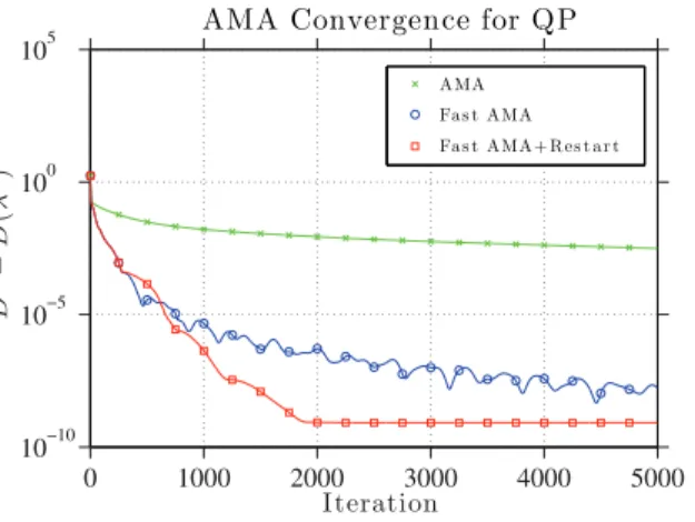
We compare the performance of five different algorithms on each test problem. We apply the original ADMM (Algorithm 1), the fast ADMM (Algorithm 7), and fast ADMM with restart (Algorithm 8). Because problem (41) is strongly convex, its dual is Lipschitz differ-entiable. For this reason, it is possible to solve the dual of (41) using Nesterov’s gradient method (Algorithm 5). We consider two variants of Nesterov’s method—the original acceler-ated method (Algorithm 5) and also a variant of Nesterov’s method incorporating a restart whenever the method becomes nonmonotone [37].
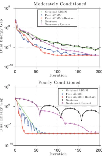
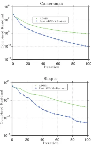
Figure 1shows sample convergence curves for the experiments described above. The dual energy gap (i.e., D(λ)−D(λk)) is plotted for each iterate. The dual energy is a natural
measure of error, because the Nesterov method is acting on the dual problem. When σe = 1,
the original ADMM without acceleration performed similarly to both variants of Nesterov’s method, and the accelerated ADMMs were somewhat faster. For the poorly conditioned problem (σe= 0.1), both variants of Nesterov’s method performed poorly, and the accelerated
ADMM with restart outperformed the other methods by a considerable margin. All five methods had similar iteration costs, with all schemes requiring between 0.24 and 0.28 seconds to complete 200 iterations.
0 50 100 150 200 10−10 10−5 100 105 Iteration D u al E n e rgy G a p Moderately Conditioned O r i g i n a l A DMM Fa s t A DMM Fa s t A DMM+ R e s t a r t N e s t e r ov N e s t e r o v+ R e s t a r t 0 50 100 150 200 10−10 10−5 100 105 Iteration D u al E n e rgy G a p Poorly Conditioned O r i g i n a l ADMM Fa s t A DMM Fa s t A DMM+ R e s t a r t N e s t e r ov N e s t e r o v+ R e s t a r t
Figure 1. Convergence curves for the elastic net problem.
One reason for the superiority of the fast ADMM over Nesterov’s method is the step-size restriction. For this problem, the step-step-size restriction for fast ADMM is τ3 ≤ λ22σH,
whereσH is the minimal eigenvalue ofMTM.The step-size restriction for Nesterov’s method is τ ≤ (λ2+σH−1)−1, which is considerably more restrictive when M is poorly conditioned
and σH is small. For the moderately conditioned problem ADMM is stable with τ ≤0.906,
while Nesterov’s method requiresτ ≤0.213.For the poorly conditioned problem, fast ADMM required τ ≤0.201, while Nesterov’s method requiredτ ≤0.0041.
7.2. Image restoration. A fundamental image processing problem is image restoration/ denoising. A common image restoration model is the well known total variation or Rudin– Osher–Fatemi [44] model:
(42) minimize |∇u|+μ2u−f2.
Note that we use the discrete forward gradient operator ∇:RΩ →RΩ×R2, which is defined entrywise as
(∇u)i,j = (ui+1,j−ui,j, ui,j+1−ui,j),
and denote the discrete total variation of uas simply|∇u|.When f represents a noisy image, minimizing (42) corresponds to finding a denoised imageuthat is similar to the noisy imagef
while being “smooth” in the sense that it has small total variation. The parameter μcontrols the tradeoff between the smoothness term and the fidelity term.
To demonstrate the performance of the acceleration scheme, we use three common test images: “cameraman,” “Barbara,” and “shapes.” Images were scaled with pixel values in the 0–255 range and then contaminated with Gaussian white noise of standard deviation σ= 20.
To put the problem in the form of (1), we takeH(u) = μ2u−f2, G(v) =|v|, A=∇, B =−I,
and b= 0.We then have the formulation
minimize μ2u−f2+|v|
subject to ∇u−v= 0
over u∈RNu and v∈RNv. For this problem, we have σH =μand ρ(ATA) =ρ(ΔTΔ)<8. The step-size restriction for Algorithm 9is thus τ < μ/8.
Using this decomposition, steps 2 and 3 of Algorithm 9 become
uk=f − 1 μ(∇ · ˆ λk), vk= shrink ∇uk+τλˆk,1 τ , (43)
where the shrink operator is defined in (2). Note that both the u and v update rules involve only explicit vector operations including difference operators (for the gradient and divergence terms), addition, and scalar multiplication. For this reason, the AMA approach for image denoising is easily implemented in numerical packages (such as MATLAB), which is one of its primary advantages.
For comparison, we also implement the fast ADMM method with restart using τ =μ/2,
which is the step size suggested for this problem in [22]. To guarantee convergence of the method, the first minimization substep must be solved exactly, which can be done using the fast Fourier transform (FFT) [22]. While the ADMM method allows for larger step sizes than AMA, the iteration cost is higher due to the use of the FFT rather than simple differencing operators.
Experiments were conducted on three different test images: “cameraman,” “Barbara,” and “shapes.” Images were scaled from 0–255, and a Gaussian noise was added with σ = 20 and σ= 50.Images were then denoised withμ= 0.1,0.05 andμ= 0.01, respectively. Sample noise-contaminated images are shown in Figure 2. Denoising results for the case σ = 20 are shown in Figure 3. Iterations were run for each method until they produced an iterate that satisfied uk−u/u<0.005.Below each image we display the unaccelerated/accelerated
iteration count for AMA (top) and ADMM (bottom).
A more detailed comparison of the methods is displayed in Table1, which contains iteration counts and runtimes for both AMA and ADMM. Note that ADMM was advantageous for very coarse scale problems (small μ), while AMA was more effective for large values of μ. This is expected, because the AMA implementation uses only first-order difference operators, which moves information through the image slowly, while ADMM uses the Fourier transforms, which moves information globally and resolves large smooth regions quickly.
(a) (b) (c)
Figure 2. “Cameraman” test image. (a)Original image. (b)Gaussian noise, σ= 20.(c)Gaussian noise,
σ= 50.
Note also that all four methods were considerably slower for smallerμ.However, this effect is much less dramatic when accelerated methods are used.
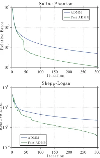
7.3. Fast split Bregman method for compressed sensing and deblurring. In this sec-tion, we consider the reconstruction of images from measurements in the Fourier domain. A common variational model for such a problem is
(44) minimize |∇u|+2∇u2+μ2RFu−f2
over u∈RNu, whereF denotes the discrete Fourier transform,R is a diagonal matrix, andf represents the Fourier information that we have obtained. The data term on the right enforces that the Fourier transform of the reconstructed image be compatible with the measured data, while the total variation term on the left enforces image smoothness. The parameter μ medi-ates the tradeoff between these two objectives. We also include an2 regularization term with parameter to make the solution smoother and to make the fast ADMM more effective. We consider two applications for this type of formulation: image deconvolution and compressed sensing.
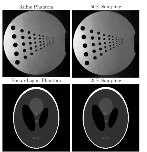
The reconstruction of an image from a subset of its Fourier modes is at the basis of mag-netic resonance imaging (MRI) [1, 28]. In classical MRI, images are measured in the Fourier domain. Reconstruction consists simply of applying the inverse FFT. Renewed interest in this area has been seen with the introduction of compressed sensing, which seeks to reconstruct high-resolution images from a small number of samples [8,7]. Within the context of MRI, it has been shown that high-resolution images can be reconstructed from undersampled infor-mation in the Fourier domain [29]. This is accomplished by leveraging the sparsity of images; i.e., the reconstructed image should have a sparse representation. This imaging problem is modeled by (44) if we choose R to be a diagonal “row selector matrix.” This matrix has a 1 along the diagonal at entries corresponding to Fourier modes that have been measured, and 0’s for Fourier modes that are unknown. The known Fourier data is placed in the vector f.
The next application we consider is image deblurring. In many imaging applications, we wish to obtain an image u from its blurred representation ˜u = K ∗u, where K represents
16/9 21/10 76/23 17/10 2839/162 178/112 15/9 23/10 68/22 15/9 1914/135 120/77 16/9 17/9 92/24 14/9 4740/184 296/171
Figure 3. Iteration count versus image scale. Images were denoised withμ= 0.1(left),μ= 0.05(center), and μ = 0.01 (right) to achieve varying levels of coarseness. The number of iterations required to reach a relative error tolerance of5×10−3 is reported below each image for both the fast/slow methods, with AMA on top and ADMM below.