A Comparison of Three Probabilistic Models of
Binary Discrete Choice Under Risk
by
Nathaniel T. Wilcox
* AbstractThis paper compares the “out-of-context” predictive success of three probabilistic models of binary discrete choice under risk. One of the models is the conventional homoscedastic latent index or “strong utility” model that is widespread in applied econometrics: This model is
“context-free” in the sense that its error part is homoscedastic with respect to decision sets. The other two models are also latent index models, but their error part is heteroscedastic with respect to decision sets, and in that sense are “context-dependent” models. Context-dependent models of choice under risk arise from several different theoretical perspectives. Here I consider my own “contextual utility” model (Wilcox 2009) and the “decision field theory” model (Busemeyer and Townsend 1993). A new experiment is performed on 80 subjects. Two-thirds of the data is used to estimate models at the individual level, and these estimates are used to predict the remaining third of choices. The data is divided up so that the decision sets in the estimating data and the prediction data have interestingly different contexts. The context-dependent error models consistently outperform the context-free error model in prediction.
JEL Classification Codes: C25, C91, D81
Keywords: risk, discrete choice, probabilistic choice, heteroscedasticity, prediction. Preliminary Draft, March 2010. Please do not cite without asking me.
Beginning with Mosteller and Nogee (1951), dozens of experiments on discrete choice under risk established that discrete choice under risk appears to have a strong probabilistic, random or stochastic component. These experiments involve repeated trials of binary choice pairs, and reveal substantial choice switching by the same subject between trials. In some cases, the trials span days (e.g. Tversky 1969; Hey and Orme 1994; Hey 2001) and one might worry that decision-relevant conditions may have changed between trials. Yet similarly substantial switching occurs even between trials separated by bare minutes, with no intervening change in wealth, background risk, or any other obviously decision-relevant variable (Camerer 1989; Starmer and Sugden 1989; Ballinger and Wilcox 1997; Loomes and Sugden 1998).
Since Kahneman and Tversky (1979) introduced Prospect Theory, most research on choice under risk has concerned its “structure,” that is the functional form or “representation” that describes how lottery characteristics (outcomes, events and their likelihoods) are
functionally combined to represent binary preference directions. Econometrically, that discussion concerns the functional form taken by the fixed part of the latent index in a traditional discrete choice model. However, there is resurgent interest in the stochastic part of decision under risk. This has been driven both by theoretical questions and empirical findings. Theoretically, some or all of what passes for “an anomaly” (say, an apparent violation of expected utility or EU theory) can be attributed to stochastic models rather than the structure in question (Wilcox 2008). This old point goes back at least to Becker, DeGroot and Marschak’s (1963a,1963b) observation that violations of the “betweenness” property of EU are precluded by some probabilistic versions of EU (random preferences) but allowed by others (strong utility). But this general concern has been resurrected by many writers; Loomes (2005), Gul and Pesendorfer (2006) and Blavatskyy
In this paper I compare three probabilistic models of choice under risk. One of the models is the conventional homoscedastic latent index or “strong utility” model that is widespread in applied econometrics: This model is “context-free” in the sense that its random part is
homoscedastic with respect to decision sets. The other two models are also latent index models, but their error part is heteroscedastic with respect to decision sets, and in that sense these two models are “context-dependent.” Context-dependent models of choice under risk arise from several different theoretical perspectives. Here I consider my own “contextual utility” model (Wilcox 2009) and the “decision field theory” model of Busemeyer and Townsend (1993). A new experiment is performed on 80 subjects. Two-thirds of the data is used to estimate models at the individual level, and these estimates are then used to predict the remaining third of choices. The data is divided up so that the decision sets in the estimating data and the prediction data have interestingly different contexts. The context-dependent error models consistently outperform the context-free error model in prediction.
1. Preliminaries
In my experiment, each choice pair is a set of two options , , , , . The option safe pays m dollars with certainty, while the option risky pays h dollars with
probability q and l dollars with probability 1 , where . Subjects choose between risky and safe in each pair presented to them. I call the vector of outcomes , , the context of each pair. Figure 1 shows an example pair where , 90,1/6,40 , 50 and the context of the pair is 40,50,90 . One familiar interpretation of each specific context is that it names a specific Machina/Marschak triangle (see e.g. Machina 1987) representing all possible
pairs of lotteries composed solely from the three possible outcomes 40, 50 and 90. Figure 2 shows this representation of the example pair in a Machina/Marschak triangle.
I consider a class of probabilistic choice models of the form
(1) , ) , ( ) ( ) ( ) Pr( safe risky D safe V risky V F risky P
where V(risky)V(safe) is a decision-theoretic representation of the difference between the values of the options risky and safe, is a scale (or inverse standard deviation) parameter,
) , (risky safe
D is an adjustment to the scale parameter in heteroscedastic models, and F is a
cumulative distribution function or c.d.f. where F(0) = 0.5 and F(x) = 1−F(−x).
While my focus is on assumptions about the function D(risky,safe), I first discuss the “value difference” V V(risky)V(safe). The function V needs to be a decision-theoretic representation of lottery value with theoretical breadth and empirical strength. Rank-dependent utility or RDU, developed by Quiggin (1982), Chew (1983) and many others, fits this bill. Under RDU, the values of two-outcome options like risky, and single outcome options like safe, are
(2) Vrisky w(q)u(h)[1w(q)]u(l) and Vsafe u(m), where
) (z
u is the utility of outcome z; and
) (q
w is the weight associated with the probability q of receiving the highest outcome h
in the pair {risky,safe}.
RDU nests the expected utility or EU representation: EU is just that special case of RDU where
q q
w( ) . Therefore we develop all choice models below in terms of RDU. To convert those
into EU-based models, just replace w(q) by q in 3 to get
(4) EU qu(h)(1q)u(l)u(m), the EU value difference between risky and safe.
Special experimental design choices also make the RDU representation indistinguishable from both Tversky and Kahneman’s (1992) cumulative prospect theory (or CPT) and Savage’s (1954) subjective expected utility (or SEU) representation. Cumulative prospect theory differs from RDU only in its treatment of negative outcomes or, more correctly, outcomes below some reference point (put differently, CPT posits loss aversion), and my experiment pairs contain only large positive outcomes of $40 to $120. In general, RDU is not a subjective expected utility model since the weight associated with an outcome will in general change when the rank order of an outcome differs in two different lotteries, regardless of whether the event(s) generating that outcome are held constant across those two lotteries. But if the mapping between events and outcome ranks is held constant across all lotteries, then SEU is indistinguishable from RDU. My experimental pairs intentionally satisfy this requirement as well.1
This implies that the RDU representation in eq. 2 will be very broad, equivalent to (or nesting) all of RDU, CPT, SEU, EU and EV (expected value). If we wished to distinguish
between these representations, this deliberate confounding would be a bug, but here it is a feature
1 More concretely: In the experiment, lotteries risky all have probabilities q of receiving their high outcome that are in sixths, generated by the roll of a six-sided die. All lotteries are constructed so that q = k/6 is always the roll “1 or 2 or…k”. So w(k/6), the weight on the high outcome h in risky, can always be thought of as the subjective
since my interest lies with the scale adjustment D(risky,safe). By experimental design, the RDU representation of V V(risky)V(safe)will encompass this wide set of decision-theoretic representations, so all inferences concerning D(risky,safe) will be robust for this set of decision-theoretic representations.
Decision theory knows the first probabilistic model as the “strong utility” or SU model (Debreu 1958; Block and Marschak 1960; Luce and Suppes 1965), and econometrics knows this as the homoscedastic latent index model. It imposes the restriction D(risky,safe)1 on eq. 1, and with RDU it is
(5) Prdsu Pr(risky)F(RDU).
As is well-known (Luce 1959 ), if we choose the logistic c.d.f. (x) as F(x), this is equivalent to a binary logit with RDU lottery values:
(6) ) exp( ) exp( ) exp( ) Pr( safe risky risky rdsu V V V risky P
, with Vrisky and Vsafe as given in eq. 2.
McFadden and others developed this model in economics, and it appears widely in
experimental/behavioral applied theory (e.g. McKelvey and Palfrey 1995; Camerer and Ho 1999). I use the logistic c.d.f. as F in all my estimations for this reason, so that my results speak clearly to these applications.
(7) ) ( ) (h u l u RDU F Prdcu .
Contextual utility makes comparative risk aversion properties of the RDU representation and its stochastic implications consistent within and across contexts. For representations such as RDU and EU, utility functions u(z) are only unique up to a ratio of differences: Intuitively, contextual utility exploits this uniqueness to create a correspondence between structural and stochastic definitions of comparative risk aversion. To see this, consider any pair on a context. Under RDU and contextual utility, the choice probability in eq. 7 can be rewritten as
(8) Prdcu F
[(l,m,h)w(q)]
, where (l,m,h)[u(m)u(l)]/[u(h)u(l)].This probability is decreasing in the ratio of differences (l,m,h). Consider two subjects Anne and Bob: Assume that they have identical weighting functions (which includes the case where both have EU preferences) and identical scale parameters . Also assume that Bob is globally more risk averse than Anne in Pratt’s sense—that Bob’s local absolute risk aversion
) ( / ) (z u z u
exceeds that of Anne for all z. The latter assumption, and simple algebra based on Pratt’s (1964) main theorem, then implies that Bob(l,m,h)Anne(l,m,h), on all contexts, and as a result (8) implies that Bob will have a lower probability than Anne of choosing risky on all contexts. Wilcox shows that it is mathematically impossible for strong utility to share this property, and this is the primary motivation behind the contextual utility model.
(9) )] ( 1 )[ ( )] ( ) ( [u h u l w q w q RDU F Prddft .
Note that eq. 9 is DFT only for pairs like those found in this experiment, where every pair consists of a two-outcome risk versus a sure outcome. In general, the function D(risky,safe) varies in a complex but theoretically well-specified manner with decision sets. Notice too that in this special case DFT shares CU’s main property: Holding constant scale parameters and
weighting functions, globally greater risk aversion (in the sense of Pratt) will imply a lower probability of choosing risky in all pairs on all contexts. DFT has another attractive property: As q approaches zero (or one)—that is, as safe (or risky) gets closer to stochastically dominating risky (or safe)—the probability of choosing the (nearly) stochastically dominating alternative approaches certainty.
Busemeyer and Townsend (1993) derive decision field theory from a sophisticated computational logic, but a simple intuition can be given for the model. Suppose that a decision maker’s computational resources can effortlessly and quickly provide utilities of outcomes, and also suppose the decision maker wishes to choose according to relative RDU value; but suppose she does not have an algorithm for effortlessly and quickly multiplying utilities and weights together. The decision maker could proceed by sampling the possible utilities in options in proportion to their decision weights, keeping running sums of these sampled utilities for each option, and stop (and choose) when the difference between the sums exceeds some threshold determined by the cost of sampling. In essence, the choice probability in eq. 9 results from this kind of sequential sampling decision procedure, which can be traced back to Wald (1947).
The superscripts in eqs. 5, 7 and 9 (rdsu, rdcu and rddft) index specific combinations of a decision-theoretic representation and a stochastic model: The prefix rd denotes a latent index based on the RDU representation, while the suffixes su, cu and dft denote the three probabilistic models. Corresponding EU-based denotations are eusu, eucu and eudft. Call these specifications, and let spec stand for any one of them. The purpose of this study is to compare the “out-of-context” predictive power of these specifications. The next section describes the experiment that collects the data for this purpose. After that, we will return to comparing the specifications.
2. Experimental Design and Protocol
The subjects in this summer 2008 experiment were 80 University of Houston undergraduate students, recruited widely from registered students by means of a single undergraduate listserv email announcement. Each subject was individually scheduled for three separate sessions on three separate days of their own choosing, almost always finishing all three sessions within one week. Only one subject had to be replaced due to noncompletion of the three-day protocol. On each day, each subject made choices from the 100 choice pairs shown in Table 1, so that each made 300 choices in all by the end of their third day. On each day, the 100 choice pairs were split into two halves of 50 pairs each, separated by about ten to fifteen minutes of other tasks (demographic surveys, item response surveys, short tests of arithmetic and problem-solving ability, and so forth). Only rarely did any day’s session last more than an hour, and most sessions were substantially shorter than this. At the conclusion of each subject’s third day, one of their 300 choice pairs was selected at random (by means of the subject drawing a ticket from a bag) and the subject was paid according to their choice in that pair (this is called random task selection). If the subject’s choice in the selected pair was risky, the subject selected a six-sided
die from a box of six-sided dice (rolling them until satisfied if they wished), and their selected die was then rolled by the attendant to determine the payment.
Here is the reasoning behind the protocol’s features. I want to estimate utilities and weights without aggregation assumptions. Decision theories are about individuals, not aggregates, and aggregation mutilates and destroys many observable properties of decision theories (Wilcox 2008). A large amount of choice data from each subject is needed to estimate utilities and weights with any precision at the individual level. A subject will become bored, and will become careless, if she makes hundreds of decisions at one sitting. So the decisions are divided up across three days, and on each day into two parts separated by unrelated tasks providing a break from decisions. The separation across three days, in particular, introduces a risk that some substantial event altering a subjects’ wealth or background risks will occur between days, which could arguably undermine the assumption that utilities of outcomes and hence choice probabilities are stationary throughout the protocol. This is a risk I am willing to run to mitigate subject boredom with hundreds of choice tasks, and I can check whether
distributions of risky choice proportions across subjects appear to be stationary across subjects’ three days of decisions. Figure 3 shows these distributions. Although the first day distribution appears to have slightly less dispersion, no parametric or nonparametric test finds any significant difference between these three daily distributions. The within-subject difference between risky choice proportions on the first and third day has a zero mean by all one-sample tests. Finally, the first principal component of risky choice proportions on the three days accounts for 95% of their collective variance, with no remotely significant second principal component associated with any particular day. There is no sign of nonstationarity of choice probabilities across the three days.
Random task selection is meant to result in truthful, motivated and unbiased revelation of preferences in each pair: That is, subjects should make each of their 300 choices as if it was the only choice being made, for real, and there should be no portfolio or wealth effects making choices interdependent across the tasks. Both the independence axiom of EUT and the “isolation effect” of prospect theory would imply this. To see this for EUT, notice that the independence axiom in its “unreduced compounds” form implies
(risky with Prob = 1/300; Z with Prob = 299/300)
if and only if
(safe with Prob = 1/300; Z with Prob = 299/300)
…where Z is any other outcome or risk, including the “grand lottery” created by the subject’s other 299 choices over the course of this experiment. Therefore, if subjects’ preferences satisfy independence in this unreduced compounds form, random task selection should be incentive compatible. Direct evidence does suggest that preferences generally satisfy the independence axiom in its unreduced compounds form (Kahneman and Tversky 1979; Conlisk 1989).
Moreover, empirical examinations of random task selection in binary lottery choice experiments find no systematic choices differences between tasks selected with relatively low or high
probabilities (Wilcox 1993) nor between tasks presented singly or under random task selection (Starmer and Sugden 1991), at least for relatively simple tasks like the pairs used here.
Two competing issues surround the resolution of risky lottery outcomes. On the one hand experimenters want random devices to be concrete, observable and credible. This is why we use dice, cards, bingo cages and so forth. We also want subjects to have good reason to believe these
devices are not rigged against them: This is why subjects select a die from an offered box of dice (and, if they wish, after rolling several to “test” them). However, the experimenter rolls the selected die because subjects may believe they exercise control over the die (whether they truly can or not; see e.g. Langer 1982). Here, the protocol compromises between the desire for credibility of randomizing devices and the possibility of subject beliefs in control over the die.
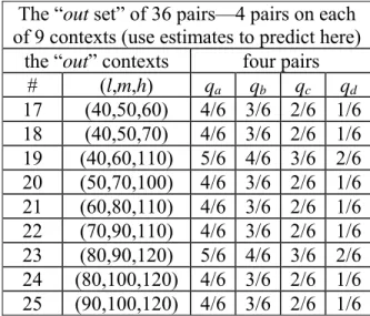
The choice pairs in Table 1 are organized into groups of four tasks (the rows of the table) by their shared outcome context. All risky lotteries are chances q and 1-q (in sixths, generated by a six-sided die) of receiving the high and low outcomes h and l on the context, respectively: Four values of q shown in each row in Table 1 (qa, qb, qc and qd) create four risky lotteries on each context, and each of these is paired with safe (the middle outcome m of the context with certainty) to create four pairs on the context. There are twenty-five distinct contexts, all constructed from nine positive money outcomes ($40 to $120 in $10 increments).
Multiple outcome contexts serve several purposes. Nonparametric identification of all utilities and weights is impossible unless the same events (the die rolls) are matched with a multiplicity of outcomes on different contexts. My nonparametric ambitions here are high: In principle, I want to be able to estimate the utilities and weights without functional form assumptions. Multiple contexts improves the separate identification of utilities and weights. Additionally, the major difference between the context-free strong utility or SU model and the context-dependent DFT and CU models is how the latter models depend on u(h)u(l)through the D(risky,safe) function. Therefore, the design deliberately creates a wide variety of contexts so that u(h)u(l) is expected to vary widely across contexts: For instance, monotonicity of utilities in outcomes z implies that u(h)u(l) must be greater on the context (40,60,110) than on
the context (50,70,100) (these are contexts 19 and 20 in Table 1, respectively). This kind of variation is key to distinguishing between the probabilistic models.
Note also that Table 1 divides the 25 contexts (and hence the 100 pairs) into two disjoint sets of contexts—the “in” set of 16 contexts (64 pairs) on the left, and the “out” set of 9 contexts (36 pairs) on the right. For prediction comparisons, I estimate specifications using each subject’s choices from the in choice pairs (this is 64 pairs, for 192 observations over three days), and use these estimates to predict each subject’s choices from the “out” pairs (this is 36 pairs, for 108 choices over three days). The prediction is, therefore, an “out-of-context” prediction since the contexts of the in pairs and the out pairs are wholly distinct.
Finally, the choice of “sixths” as the “probability unit” for constructing risks serves several purposes. First, the six-sided die is perhaps the most culturally familiar randomizing device: This reduces some of the artificiality of laboratory risks. Second, sixths are well-suited to revealing a widely-believed shape of weighting functions. Figure 4 shows Prelec’s (1998) single-parameter weighting function w(q|)exp([ln(q)]) q (0,1), w(0)=0 and w(1)=1, at various values of from 0.5 to 1, covering widely-held priors about the shape of the function. The linear function (heavy black line) is EU with = 1. Figure 4 shows that the maximum downward deflection of the nonlinear versions (from linearity) occurs very close to q = 5/6; and at q = 1/6 the upward deflection of nonlinear versions is about 75% of its maximum (which generally occurs at a somewhat smaller q). Finally, Monte Carlo simulations suggested that relatively coarse probability grids (fourths or sixths) over many different contexts permits relatively more precise estimation of utilities and weights.
3. Estimation
To discuss the estimation, it is helpful to define indices for pairs, trials (days) and subjects, as well as some important sets of indices:
i = 1,2,…I, indexing I distinct pairs. Here I = 100.
Pairs i are then {(hi,qi,li),mi}, or {riskyi,safei}; and also note that i = 1 to 64 are the in pairs, and i = 65 to 100 are the out pairs, in Table 1.
t = 1,2,…T, indexing T distinct trials (days) of each pair. Here T = 3 (the three days). s = 1,2,…S, indexing the S distinct subjects. Here S = 80.
it: A double subscript indicating the tth trial of choice pair i. 1
s it
r if subject s chose riskyi in her tth trial of pair i, and zero otherwise. )
| (rits it set s
set
r , the observed choice vector of subject s over those pairs and trials in set. The set will be in, out or all, where in = { it | i 64 } (the estimation pairs/trials), out = { it | i 65 } (the prediction pairs/trials) and all = {all it} is all 300 pairs/trials.
Let us(z) and ws(q) denote utilities of outcomes z and weights associated with probabilities q, respectively, of subject s. The experiment involves nine distinct outcomes
] 120 ,$ 110 ,...,$ 50 ,$ 40 [$
z across its 100 choice pairs, so there are nine utilities
)] 120 ( ), 110 ( ),..., 50 ( ), 40 ( [ s s s s u u u
u for each subject s.
Because of the affine transformation invariance property of RDU and EU utilities, we can arbitrarily choose s(40)0
)] 120 ( ), 110 ( ),..., 70 ( ), 60 ( [ s s s s s u u u u u .
The nonparametric treatment of utility makes each of those seven utilities a separate parameter to be estimated. I also examine a 2-parameter parametric alternative, the expo-power function (Saha 1993, Holt and Laury 2002) which blends the CARA and CRRA utilities in a flexible way,
…normalized so that s(40)0
u and us(50)1. The experiment also involves five distinct probabilities q[1/6,2/6,3/6,4/6,5/6], so there is a vector ws of five weights to be estimated for each subject,
)] 6 / 5 ( ), 6 / 4 ( ), 6 / 3 ( ), 6 / 2 ( ), 6 / 1 ( [ s s s s s s w w w w w w .
The nonparametric approach again makes each of those five weights a separate parameter to be estimated. There are several parametric weighting functions in the literature such as the Prelec (1998) one-parameter function discussed above, but none are very flexible. Instead, I use the Beta distribution’s c.d.f. (with two parameters and ) as my parametric alternative, that is
| , .
It is the right kind of function (taking the unit interval onto itself, and monotone increasing) from the viewpoint of the general RDU representation theorem. It is much more flexible and
(importantly) can take all major shapes suggested by the theorists who developed RDU and/or Cumulative Prospect Theory. It is also easily called in most nonlinear optimization software.
To summarize, the nonparametric latent index of the RDU representation, for subject s and pair i, is (10) )( , ) ( ) ( ) [1 ( )] ( ) ( i s i s i s i s i s s s i w q u h w q u l u m RDU u w , where )] 6 / 5 ( ), 6 / 4 ( ), 6 / 3 ( ), 6 / 2 ( ), 6 / 1 ( [ s s s s s s w w w w w w ,
Combining 10 with 5, 7 and 9, and choosing the logistic c.d.f. as F(x), we have the following choice probability specifications:
(11) ( , , )
( s, s)
i s s s s rdsu i RDU P u w u w . (12) ) ( ) , ( ) , , ( cu s i s s i s s s s rdcu i D RDU P u w u w u , where Dicu(us)us(hi)us(li). (13) ) , ( ) , ( ) , , ( rddft s s i s s i s s s s rddft i D RDU P w u w u w u , where )] ( 1 )[ ( )] ( ) ( [ ) , ( s i i s i s i s s s rddft i u h u l w q w q D u w Corresponding EU-based choice probabilities with either the strong utility or contextual utility model simply omit the vector of weights s
w from the function arguments and, in the case of DFT, set s i i
q q
w ( ) in the denominator expression.
Equations 10-13 define the probability of the event s 1 it
r (subject s chose risky in the tth trial of pair i). Letting spec( s, s, s)
i
P u w generically denote any of those probabilities, the generic log likelihood of s it r , given (us,ws,s), is (14) )]( | , , ) ln[ ( , , )] (1 )ln[1 spec( s, s, s i s it s s s spec i s it s s s s it spec P r P r r u w u w u w .
and estimation of s ( s, s,s)
w u
by maximum likelihood, for each subject, is straightforward. Beginning with Manski (1975), econometricians made substantial progress eliminating the need for choosing a specific c.d.f. for F(x) in latent index models (e.g. Cosslett 1983; Klein and Spady 1993; Lewbel 2000). To my knowledge, none of these innovative methods can work with the fully nonparametric latent index of RDU (as in eq. 10). In essence, all “regressors” in eq. 10 are dummy variables (or interactions of dummy variables) indicating the presence or absence of particular outcomes and events in any pair i. As is well-known in this literature, dispensing with knowledge of F(x) requires a so-called “special regressor” with several necessary properties: In particular, the special regressor must have an absolutely continuous distribution. I do not believe dummy regressors and their interactions, as in eq. 10, have that property, so I don’t believe I can use these innovative methods here. Moreover, in DFT, the logistic distribution arises as the limiting distribution of the sequential sampling process as the time interval between samples gets small, and this is a maintained assumption of DFT
(Busemeyer and Townsend 1993). In other words, the choice of the logistic c.d.f as F(x) has a good theoretical motivation, at least from the perspective of one of the probabilistic models.
There is some interest in estimating s ( s, s,s)
w u
using all of the data. This is particularly true for the fully nonparametric latent index models, since these provide a first look at function-free utilities and weights estimated simultaneously from discrete choice data. (I do not think this has been done before.) But for the purpose of comparing the probabilistic models, I prefer to compare their “out-of-context” prediction quality. To do that, I estimate s using just the in data, and use this estimate to predict choices on the out data. Let s
in
r and routs denote the in and out choice vectors for each of the 80 subjects s. Estimate each specification using just the
specifications spec1 and spec2, for each s. Then using these estimates, the out set of data s out r , and eq. 15, we can calculate log likelihoods of the predictions based on the in set estimates,
(16) 1( ) 1( | ˆspec1,s) in s out spec spec out s r , and 2( ) 2( | ˆspec2,s) in s out spec spec out s r .
I use Vuong’s (1989) test to compare these prediction log likelihoods for pairs of specifications spec1 and spec2. It allows non-nested specifications and neither needs to be “correct” (the test is against the null “The specifications are equally close to the true DGP”). Intuitively, the test treats differences between the log likelihoods of two specifications as normal variates and does a z test on them. Define
) ( ) ( ) 2 , 1 ( 1 2 s s spec
spec specout specout s out ,
( 1, 2) s801 s ( 1, 2)/80 outout spec spec spec spec , and
( 1, 2) ( 1, 2)
/80 ) 2 , 1 ( 80 1 2
s out s outout spec spec spec spec spec spec
SD .
Vuong’s test statistic is then
(17)
80 / ) 2 , 1 ( ) 2 , 1 ( ) 2 , 1 ( spec spec SD spec spec spec spec z out out out 4. Results
Table 2 shows the seven representations (and treatments of utilities and/or weights) that I combine with the three probabilistic models to generate twenty-one specifications. All seven representations of the latent index are nested within eq. 10, the fully nonparametric RDU latent index. By restricting eq. 10 to have either linear weights, linear utilities or both, we get
(respectively) expected utility or EU, Yaari’s (1987) Dual Theory or “Yaari,” and expected value. RDU, EU and Yaari may be further restricted by replacing the nonparametric treatment of their utilities and/or weights by the 2-parameter functions discussed earlier (the expo-power function for utilities and/or the Beta c.d.f. for weights).
Figures 5 and 6 graph the 80 weight and utility functions (respectively) estimated using all of the data, the fully nonparametric RDU latent index in eq. 10, and the eq. 12 (CU)
probability model. Figure 6 shows that the vast majority of utility functions are uniformly concave with perhaps a handful of exceptions. However, Figure 5 makes it clear that there is great heterogeneity of weight function shapes, so both Figures 5 and 6 employ a common color-coding for subjects with salient weight function shapes. Comparing Figures 4 and 5, it is curious but true that very few of the estimated weight functions appear to have the characteristic inverse-s inverse-shape poinverse-sited by many theoriinverse-stinverse-s. In Figure 5, thiinverse-s expected inverse-shape iinverse-s coded green: Although 14 of 80 weight functions have this general shape, most of those 14 cross the diagonal at a relatively high q above one-half, which is not true (for instance) of the one-parameter Prelec (1998)
function shown in Figure 4 (this function always crosses the diagonal at 0.37). The plurality of estimated weight functions (30 of the 80, coded blue in Figure 5) are uniformly concave and above the identity weights of EU, which Quiggin (1993) calls optimism. A very small number (4 of 80, coded red in Figure 5) are uniformly convex and below identity
weights, which Quiggin calls pessimism. Finally, the second-most-common estimated weight function (26 of 80, coded orange in Figure 5) is s-shaped. One interpretation is that these people tend to “round” low probabilities to zero and high probabilities to unity, so one might call these people “approximators.”
Comparison of Figures 5 and 6 suggests an odd relationship: The blue-coded optimists (concave weight functions) also tend to have the greatest concavity of their utility functions. This sounds counterintuitive since more concave utility means greater risk aversion while more concave weights (optimism) means less risk aversion. Part of the answer to this puzzle is undoubtedly poor identification for relatively risk-averse subjects. As a subject becomes
increasingly risk-averse overall (for whatever reason), there will be less variation in her choices and separate identification of weights and utilities will be relatively poor. For such subjects, a positive finite sample correlation between estimated utility and weights concavity will be expected. Monte Carlo simulations of information matrices of relatively risk-averse RDU/CU data-generating processes confirm this econometric intuition. Therefore I suggest that this apparent finding be taken with a grain of salt.
Figure 7 displays the prediction comparisons between specifications in a graphical manner. The figure displays a linearly transformed version of average prediction log likelihoods,
(18) “Percent prediction metric” = evsu out frontier out spec out frontier out , where
s spec( )/80 out spec out s .The specification evsu is an expected value latent index with the SU probability model: This model has just one estimated parameter for each subject (the scale parameter ) and I treat this as
the best possible out-of-context prediction likelihood with stationary choice probabilities. Since the experimental design involves repeated trials, and since there is some inconsistency of subject choices across repeated trials, this best possible likelihood is nonzero for each subject, and so is its average across subjects. No model with stationary probabilities can predict better than this. If this metric takes the value 100%, the specification predicts no better than a strong utility
expected value model. If this metric takes the value 0%, the specification predicts as well as any possible specification with stationary probabilities can predict.
Figure 7 shows that specifications with 2-parameter parametric treatments of utilities and/or weights, near the center of the figure, perform best in out-of-context prediction. This is not surprising since these specifications involve many fewer parameters than the fully
nonparametric specifications. Yet even the fully nonparametric specifications at the left almost always predict noticeably better than the maximally lean EV (expected value) specifications at the far right (the sole exception here being the nonparametric Yaari representation with DFT). There are two other important findings. First, notice that holding representations constant, the context-dependent probability models CU and DFT are almost uniformly better at prediction than the context-free strong utility or SU model. Second, examine Figure 7’s comparative results for EU and RDU representations with parametric utilities and weights (near the center of Figure 7, labeled “EU 3 parms para” and “RDU 5 parms para”). Consider the 3-parameter EU
specification with strong utility as a baseline. Notice that the improvement in prediction quality associated with changing from strong utility to CU or DFT (about 12% in both cases) exceeds the improvement in prediction quality associated with adding two parameters and changing to the 5-parameter RDU specification but staying with strong utility (about 9%). This confirms Wilcox’s (2008,2009) results using the well-known Hey and Orme (1994) data set: When we ask
“what matters for prediction?” it seems that the greatest marginal gains from a strong utility and EU starting point accrue from changing the probabilistic model rather than adopting a more expansive representation such as RDU.
Tables 3 (A, B, C and D) show the results of the Vuong (1989) tests that compare the probabilistic models. Each of these tables holds the representation constant and just compares changes in probabilistic models. Tables 3-A, 3-B, 3-C and 3-D show results for expected value, expected utility, Yaari’s dual model and rank-dependent utility, respectively. The tables all have left and right panels with in-context and out-of-context comparisons of log likelihoods.
Additionally, except for table 3-A (expected value representation), the tables all have top and bottom panels showing results for the parametric and nonparametric versions of each
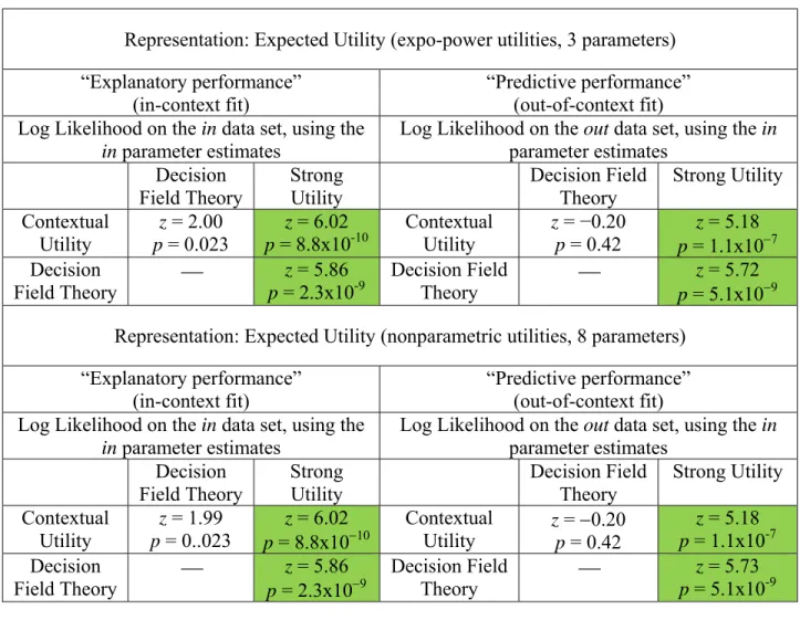
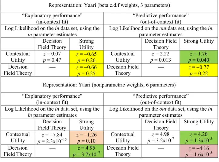
representation. With the exception of Table 3-C (the Yaari dual model representations), the Vuong tests overwhelmingly and uniformly reject strong utility in favor of both of the context-dependent probability models. Even in Table 3-C (the Yaari representation), where strong utility is occasionally directionally better than the context-dependent models, it is only significantly better in a single comparison against DFT. The contextual utility probability model is always significantly better than strong utility, regardless of the representation or parametric
expansiveness of the specifications.
The Vuong tests do not distinguish DFT and contextual utility in any consistent and persuasive way. Among the seven in-context comparisons between them, each is significantly best in three comparisons (with one insignificant comparison), and among the seven out-of-context comparisons, out-of-contextual utility significantly beats DFT in three comparisons and DFT significantly beats contextual utility in one comparison (with three insignificant comparisons).
5. Conclusions
For the purpose of predicting risky choices in new contexts, context-dependent models like contextual utility (Wilcox 2009) and decision field theory (Busemeyer and Townsend 1993) are overwhelmingly better than the traditional strong utility approach that dominates applied theoretical work in experimental and behavioral economics and much applied econometric work as well. Moreover, the greatest marginal gains in predictive success do not come from more expansive decision-theoretic representations that add parameters to be estimated: Instead they come from switching from context-free to context-dependent models, with no additional parameters to be estimated.
References
Ballinger, T. P., and N. Wilcox, 1997, Decisions, error and heterogeneity. Economic Journal 107, 1090-1105.
Becker, G. M., M. H. DeGroot and J. Marschak, 1963a, Stochastic models of choice behavior. Behavioral Science 8, 41–55.
Becker, G. M., M. H. DeGroot and J. Marschak, 1963b, An experimental study of some stochastic models for wagers. Behavioral Science 8, 199-202.
Blavatskyy, P. R., 2007, Stochastic expected utility theory. Journal of Risk and Uncertainty 34, 259-286.
Block, H. D. and J. Marschak, 1960, Random orderings and stochastic theories of responses, in I. Olkin et al., (Eds.), Contributions to probability and statistics: Essays in honor of Harold Hotelling. Stanford University Press, Stanford, pp. 97-132.
Busemeyer, J. and J. Townsend, 1993, Decision field theory: A dynamic-cognitive approach to decision making in an uncertain environment. Psychological Review 100, 432-59.
Camerer, C., 1989, An experimental test of several generalized expected utility theories. Journal of Risk and Uncertainty 2, 61-104.
Camerer, C. and T-H. Ho, 1999, Experience weighted attraction learning in normal-form games. Econometrica 67:827-74.
Chew, S. H., 1983, A generalization of the quasilinear mean with applications to the measurement of income inequality and decision theory resolving the Allais paradox. Econometrica 51, 1065-1092.
392-Cosslett, S. R., 1983, Distribution-free maximum likelihood estimator of the binary choice model, Econometrica 51, pp. 765-782
Debreu, G., 1958, Stochastic choice and cardinal utility. Econometrica 26, 440-444. Gul, F., and W. Pesendorfer, 2006, Random expected utility. Econometrica 74, 121-146. Hey, J. D., 2001, Does repetition improve consistency? Experimental Economics 4, 5-54. Hey, J. D. and C. Orme, 1994, Investigating parsimonious generalizations of expected utility
theory using experimental data. Econometrica 62, 1291-1329.
Holt, C. A. and S. K. Laury, 2002, Risk aversion and incentive effects. American Economic Review 92, 1644-1655.
Kahneman, D. and A. Tversky, 1979, Prospect theory: An analysis of decision under risk. Econometrica 47, 263-291.
Klein, R. W. and R. H. Spady, 1993, An efficient semiparametric estimator for binary response models. Econometrica 61, 387-421
Langer, E. J., 1982, The illusion of control. In D. Kahneman, P. Slovic and A. Tversky, eds., Judgment Under Uncertainty: Heuristics and Biases. New York: Cambridge University Press.
Lewbel, A., 2000, Semiparametric qualitative response model estimation with unknown heteroscedasticity or instrumental variables. Journal of Econometrics 97, 145-177.
Loomes, G., 2005, Modeling the stochastic component of behaviour in experiments: Some issues for the interpretation of data. Experimental Economics 8, 301-323.
Loomes, G. and R. Sugden, 1998, Testing different stochastic specifications of risky choice. Economica 65, 581-598.
Luce, R. D. and P. Suppes, 1965, Preference, utility and subjective probability, in R. D. Luce, R. R. Bush and E. Galanter, (Eds.), Handbook of mathematical psychology Vol. III. Wiley, New York, pp. 249-410.
Machina, M., 1987, Choice under uncertainty: Problems solved and unsolved. Journal of Economic Perspectives 1, 121-154.
Manski, C., 1975, Maximum score estimation of the stochastic utility model of choice, Journal of Econometrics 3, 205-228.
McKelvey, R. and T. Palfrey, 1995, Quantal response equilibria for normal form games. Games and Economic Behavior 10, 6-38.
Mosteller, F. and P. Nogee, 1951, An experimental measurement of utility. Journal of Political Economy 59, 371-404.
Pratt, J. W., 1964, Risk aversion in the small and in the large. Econometrica 32, 122-136. Prelec, D., 1998, The probability weighting function. Econometrica 66, 497-527.
Quiggin, J, 1982, A theory of anticipated utility. Journal of Economic Behavior and Organization 3, 323-343.
Quiggin, J, 1993. Generalized Expected Utility Theory: The Rank-Dependent Model. Norwell, MS: Kluwer.
Saha, A, 1993, Expo-Power Utility: A ‘Flexible’ Form for Absolute and Relative Risk Aversion. American Journal of Agricultural Economics 75, 905-913.
Savage, L. J., 1954. The Foundations of Statistics. New York: Wiley.
Starmer, C. and R. Sugden, 1989, Probability and juxtaposition effects: An experimental investigation of the common ratio effect. Journal of Risk and Uncertainty 2, 159-78.
Starmer, C. and R. Sugden, 1991, Does the random-lottery incentive system elicit true preferences? An experimental investigation. American Economic Review 81, 971-978. Tversky, A., 1969, Intransitivity of preferences. Psychological Review 76, 31-48.
Tversky, A. and D. Kahneman, 1992, Advances in prospect theory: Cumulative representation of uncertainty. Journal of Risk and Uncertainty 5, 297–323.
Vuong, Q., 1989, Likelihood ratio tests for model selection and non-nested hypotheses. Econometrica 57, 307–333.
Wald, A., 1947. Sequential Analysis. New York: Wiley.
Wilcox, N., 1993, Lottery choice: Incentives, complexity and decision time. Economic Journal 103, 1397-1417.
Wilcox, N., 2008, Stochastic models for binary discrete choice under risk: A critical stochastic modeling primer and econometric comparison. In J. C. Cox and G. W. Harrison, eds., Research in Experimental Economics Vol. 12: Risk Aversion in Experiments pp. 197-292. Bingley, UK: Emerald.
Wilcox, N., 2009, ‘Stochastically more risk averse:’ A contextual theory of stochastic discrete choice under risk. Journal of Econometrics doi:10.1016/j.jeconom.2009.10.012.
Table 1: The 100 Choice Pairs—the “in set” for estimation, and the “out set” for prediction. The “in set” of 64 pairs—4 pairs on each
of 16 contexts (for estimation) of 9 contexts (use estimates to predict here) The “out set” of 36 pairs—4 pairs on each the “in” contexts four pairs the “out” contexts four pairs
# (l,m,h) qa qb qc qd # (l,m,h) qa qb qc qd 1 (40,50,80) 5/6 4/6 3/6 2/6 17 (40,50,60) 4/6 3/6 2/6 1/6 2 (40,50,90) 5/6 4/6 3/6 2/6 18 (40,50,70) 4/6 3/6 2/6 1/6 3 (40,60,100) 5/6 4/6 3/6 2/6 19 (40,60,110) 5/6 4/6 3/6 2/6 4 (40,60,120) 5/6 4/6 3/6 2/6 20 (50,70,100) 4/6 3/6 2/6 1/6 5 (50,60,90) 5/6 4/6 3/6 2/6 21 (60,80,110) 4/6 3/6 2/6 1/6 6 (50,70,110) 5/6 4/6 3/6 2/6 22 (70,90,110) 4/6 3/6 2/6 1/6 7 (50,70,120) 5/6 4/6 3/6 2/6 23 (80,90,120) 5/6 4/6 3/6 2/6 8 (60,70,90) 4/6 3/6 2/6 1/6 24 (80,100,120) 4/6 3/6 2/6 1/6 9 (60,80,120) 5/6 4/6 3/6 2/6 25 (90,100,120) 4/6 3/6 2/6 1/6 10 (70,80,100) 4/6 3/6 2/6 1/6 11 (70,80,110) 5/6 4/6 3/6 2/6 12 (70,80,120) 5/6 4/6 3/6 2/6 13 (80,90,100) 4/6 3/6 2/6 1/6 14 (80,90,110) 4/6 3/6 2/6 1/6 15 (90,100,110) 4/6 3/6 2/6 1/6 16 (100,110,120) 4/6 3/6 2/6 1/6
Table 2. The seven representations estimated, including the treatment of utility and/or weigh functions and the resulting number of parameters estimated. Each of these is combined with one of the three probability models to produce twenty-one specifications in all, and each specification involves the estimation of one extra parameter, the scale parameter .
Structure Utility function treatment Weight function treatment
Expected Value (EV)
Expected Utility (EU) nonparametric (7 parms.)
Expected Utility (EU) expo-power (2 parms.)
Yaari Dual Theory (Yaari) nonparametric (5 parms.)
Yaari Dual Theory (Yaari) beta c.d.f. (2 parms.)
Rank-Dependent Utility (RDU) nonparametric (7 parms.) nonparametric (5 parms.) Rank-Dependent Utility (RDU) expo-power (2 parms.) beta c.d.f. (2 parms.)
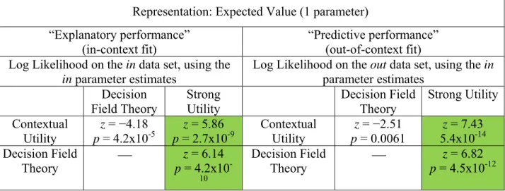
Table 3-A. Voung comparisons between the specifications: Expected value representation.
Representation: Expected Value (1 parameter) “Explanatory performance”
(in-context fit)
“Predictive performance” (out-of-context fit) Log Likelihood on the in data set, using the
in parameter estimates
Log Likelihood on the out data set, using the in parameter estimates Decision Field Theory Strong Utility Decision Field Theory Strong Utility Contextual Utility z = −4.18 p = 4.2x10⁻⁵ z = 5.86 p = 2.7x10⁻⁹ Contextual Utility z = −2.51 p = 0.0061 z = 7.43 5.4x10⁻¹⁴ Decision Field Theory z = 6.14 p = 4.2x10 -10 Decision Field Theory z = 6.82 p = 4.5x10⁻¹² Notes: All comparisons are based on parameters estimated from the 192 observations of the in data. The in-context fit comparisons compare the maximized log likelihoods of those 192 observations. The out-of-context fit comparisons use the parameter estimates to calculate log likelihoods in the out data, and compare those log likelihoods. In each cell, Vuong’s z statistic is based on the difference between the row and column probability models’ log likelihood, so negative z indicates that the column model fits best while positive z indicates that the row model fits best.
Table 3-B. Vuong comparison between the specifications: Expected utility representation. Representation: Expected Utility (expo-power utilities, 3 parameters) “Explanatory performance”
(in-context fit)
“Predictive performance” (out-of-context fit) Log Likelihood on the in data set, using the
in parameter estimates Log Likelihood on the out data set, using the in parameter estimates Decision
Field Theory Strong Utility Decision Theory Field Strong Utility Contextual
Utility p = 0.023 z = 2.00 p = 8.8x10z = 6.02 -10 Contextual Utility z = p = 0.42 −0.20 z = 5.18
p = 1.1x10⁷ Decision Field Theory z = 5.86 p = 2.3x10⁻⁹ Decision Field Theory z = 5.72 p = 5.1x10⁹
Representation: Expected Utility (nonparametric utilities, 8 parameters) “Explanatory performance”
(in-context fit) “Predictive performance” (out-of-context fit) Log Likelihood on the in data set, using the
in parameter estimates Log Likelihood on the out data set, using the in parameter estimates Decision Field Theory Strong Utility Decision Field Theory Strong Utility Contextual Utility z = 1.99 p = 0..023 z = 6.02 p = 8.8x10¹⁰ Contextual Utility z = 0.20 p = 0.42 z = 5.18 p = 1.1x10⁻⁷ Decision Field Theory p = 2.3x10z = 5.86 9 Decision Field Theory p = 5.1x10z = 5.73 -9 Notes: All comparisons are based on parameters estimated from the 192 observations of the in data. The in-context fit comparisons compare the maximized log likelihoods of those 192 observations. The out-of-context fit comparisons use the parameter estimates to calculate log likelihoods in the out data, and compare those log likelihoods. In each cell, Vuong’s z statistic is based on the difference between the row and column probability models’ log likelihood, so negative z indicates that the column model fits best while positive z indicates that the row model fits best.
Table 3-C. Vuong comparison between the specifications: Yaari’s “dual theory” representation.
Representation: Yaari (beta c.d.f weights, 3 parameters) “Explanatory performance”
(in-context fit) “Predictive performance” (out-of-context fit) Log Likelihood on the in data set, using the
in parameter estimates Log Likelihood on the out data set, using the in parameter estimates Decision Field Theory Strong Utility Decision Field Theory Strong Utility Contextual Utility z = 0.07 p = 0.47 z = 0.65 p = 0.26 Contextual Utility z = 2.22 p = 0.013 z = 1.76 p = 0.040 Decision Field Theory z = 0.66 p = 0.25 Decision Field Theory z = 0.77 p = 0.22 Representation: Yaari (nonparametric weights, 6 parameters)
“Explanatory performance” (in-context fit)
“Predictive performance” (out-of-context fit) Log Likelihood on the in data set, using the
in parameter estimates Log Likelihood on the out data set, using the in parameter estimates Decision
Field Theory Strong Utility Decision Theory Field Strong Utility Contextual
Utility p = 2.3x10z = 7.84 15 z = 1.26 p = 0.10 Contextual Utility p = 3.2x10z = 4.98 -7 p = 1.3x10z = 4.20 -5
Decision
Field Theory p = 3.7x10z = 4.95 7
Decision Field
Theory p = 1.6x10z = 4.16 -5 Notes: All comparisons are based on parameters estimated from the 192 observations of the in data. The in-context fit comparisons compare the maximized log likelihoods of those 192 observations. The out-of-context fit comparisons use the parameter estimates to calculate log likelihoods in the out data, and compare those log likelihoods. In each cell, Vuong’s z statistic is based on the difference between the row and column probability models’ log likelihood, so negative z indicates that the column model fits best while positive z indicates that the row model fits best.
Table 3-D. Vuong comparison between specifications: Rank-dependent utility representation.
Representation: Rank-Dependent Utility (expo-power utility, beta c.d.f. weights, 5 parameters) “Explanatory performance”
(in-context fit)
“Predictive performance” (out-of-context fit) Log Likelihood on the in data set, using the
in parameter estimates
Log Likelihood on the out data set, using the in parameter estimates Decision Field Theory Strong Utility Decision Field Theory Strong Utility Contextual Utility z = 4.63 p = 1.8x10⁻⁶ z = 6.63 p = 1.6x10⁻¹¹ Contextual Utility z = −0.13 p = 0.45 z = 6.35 p = 1.0x10⁻¹⁰ Decision
Field Theory p = 1.5x10z = 4.17 -5 Decision Field Theory p = 1.5x10z = 5.54 -8
Representation: Rank-Dependent Utility (nonparametric utilities and weights, 13 parameters) “Explanatory performance”
(in-context fit) “Predictive performance” (out-of-context fit) Log Likelihood on the in data set, using the
in parameter estimates Log Likelihood on the out data set, using the in parameter estimates Decision Field Theory Strong Utility Decision Field Theory Strong Utility Contextual Utility p = 0.0022z = 2.85 z = 5.82 p = 3.0x10⁻⁹ Contextual Utility z = 1.78 p = 0.037 z = 4.32 p = 7.9x10⁻⁶ Decision Field Theory p = 9.6x10z = 6.37 11 Decision Field Theory p = 0.0011z = 3.05 Notes: All comparisons are based on parameters estimated from the 192 observations of the in data. The in-context fit comparisons compare the maximized log likelihoods of those 192 observations. The out-of-context fit comparisons use the parameter estimates to calculate log likelihoods in the out data, and compare those log likelihoods. In each cell, Vuong’s z statistic is based on the difference between the row and column probability models’ log likelihood, so negative z indicates that the column model fits best while positive z indicates that the row model fits best.
Figure 1. An example pair, showing its display to subjects. The context in this example is (40,50,90) (in U.S. dollars).
Left option [“
risky
”]
Generally,
risky
is
(
h
,
q
,
l
)
,
where
h > l
,
q
= Pr(
h
) and 1
q
= Pr(
l
)…
Here,
h
= $90,
q
= 1/6 and
l
= $40.
Right option [“
safe
”]
Generally,
safe
is
m
with Prob 1,
where
h
>
m
>
l…
Figure 2. The example pair as a pair of coordinates in a Machina/Marschak triangle. example pair safe risky 0 1/6 1/3 1/2 2/3 5/6 0 1/6 2/6 3/6 4/6 5/6 1
p
h=
pro
b
a
b
il
it
y
o
f recei
v
ing
hi
g
h
o
u
tco
m
e 9
0
pl= probability of receiving low outcome 40
Example Pair in the Machina Marschak triangle
representing all pairs on its context
1ph
pl= probability of receiving middle outcome 50.Figure 3: Cumulative Distributions of Risky Choice Proportions Across Subjects, by Day. 0 25 50 75 100 0 0.25 0.5 0.75 1 Pe rc e n ta ge of 80 Su b je ct s
Proportion of Choices of Risky from the 100 Pairs
Cumulative
Distributions
of
Risky
Choice
Proportions
by
Day
day 1 day 2 day 3
Figure 4. The Prelec one-parameter weighting function with values of from 0.5 to 1.
0
0.2
0.4
0.6
0.8
1
0
0.2
0.4
0.6
0.8
1
probabilit
y
w
e
ight
on
highes
t out
c
om
e in
pair
probability of highest outcome in pair
Prelec-type one-parameter weighting functions
5/6
1/6
Figure 5: 80 individually estimated probability weighting functions. 0 0.2 0.4 0.6 0.8 1 0 0.2 0.4 0.6 0.8 1 W e ight as s o c iat ed w it h probabilit y q
Probability q of receiving high outcome in risky
Blue
= 30 “Optimists”
(above identity line).
Red = 4 “Pessimists” (below
identity line).
Green
= 14 “Prospect
Theorists” (initially above,
then below identity line).
Orange
= 26
“Approximators” (initially
below, then above identity
line).
Figure 6: 80 individually estimated utility functions, color-coded to denote weighting function type in Figure 5. 0 0.2 0.4 0.6 0.8 1 40 60 80 100 120 U tilit y of out c o m e z w it h u(40)= 0 and u(120)= 1
Outcomes z in U.S. Dollars
Blue
= 30 “Optimists” (above
identity line).
Red = 4 “Pessimists” (below
identity line).
Green
= 14 “Prospect
Theorists” (initially above,
then below identity line).
Orange
= 26 “Approximators”
(initially below, then above
identity line).
Yellow = 6 “Others” (crosses
identity line more than once).
Figure 7: Percent prediction metric for twenty-one specifications, by representation and probability model.
co
nt
ex
tu
al
dft
st
ro
ng
45
55
65
75
85
95
105
Pe
rc
en
t
Pr
ed
ic
ti
on
Me
tr
ic
(l
o
w
er
is
be
tt
er
)
Structure
(utility
function
treatment,
weighting
function
treatment)
Comparison
of
prediction
(out
‐
of
‐
sample)
negative
log
likelihoods
of
various
specifications:
Average
of
individual
estimations