REMOVAL OF DIFFERENT TYPES OF ARTIFACTS AND
IMPULSE NOISE IN GRAY SCALE IMAGES
1 S.SURESH KUMAR, 2 DR. H. MANGALAM
1
Assistant Professor, Department of ECE, Coimbatore
Institute of Engineering and Technology, Tamilnadu, India
2
Professor and Head, Sri Krishna College of Engineering & Technology,
Tamilnadu, India
E-mail: [email protected], [email protected]
ABSTRACT
An adaptive based artifacts removal algorithm is proposed for removal of blocking artifacts, strip lines, drop lines, blotches and impulses in images. The algorithm detects noise variance level and then proper method is selected depending upon the variance. The algorithm changes the maximum size of window during the filtering operation depending on noise level. The output of the filter is a particular value which replaces the current pixel value at that point on which the value is centered at that time. Thus window size is automatically modified based on the density of noise in the image. It replaces a number of independent algorithms required for removal of blocking and other different artifacts and gives better result. The performance of the algorithm is evaluated in terms of Mean Square Error (MSE), Peak Signal to Noise Ratio (PSNR), Correlation, Feature Similarity (FSIM), Mean Structural Similarity (MSSIM) and Visual signal-to-noise ratio (VSNR). The computation time is compared with other algorithms that already exist.
Keywords: Strip Lines, Blotches, Blocking Artifacts, Noise Variance, Adaptive Based Artifact Removal Algorithm, Feature Similarity.
1. INTRODUCTION
It is proven that linear filters are not quite effective in the presence of non Gaussian noise. At present, some of the limitations of linear filters are overcome by non-linear filters [1].Simple median filters (SMF) are a class of non linear filters and had produced excellent results when linear filters had generally failed [2].The main advantage of median filters is removal of impulse noise with no information loss of edge information. In remote sensing, white and black strip lines, blotches and drop lines and impulse noise occur along with the results of an aggressive data compression scheme applied to an image that discards some data that is determined by an algorithm to be of lesser importance to the overall content but which is perceptible and objectionable to the client. Compression artifacts occur in many common file formats such as Joint Pictures Experts Group (JPEG) and Moving Pictures Experts Group (MPEG). Standard median
filters are not useful to remove these artifacts. This paper describes the adaptive based artifacts removal (ABAR) algorithm to remove all blocking and various artifacts. This paper is organized as follows. Section 2 discusses the previous work. Section 3 discusses the proposed method to remove impulse noise, blocking and various artifacts. Section 4 compares the results of the proposed work with other techniques and Section 5 gives the conclusion.
2. RESEARCH BACKGROUND
does not work properly. Due to disturbing microwave energies in the sensors, impulse noises appear and make the system to degrade continuously. To overcome these artifacts, generally different methods are employed. According to Corte-Real et al [4], a positive type film is suffered from bright scratches and a negative type film is suffered from dark scratches. It gives a solution to remove the blotches and line scratches in images but considered only vertical narrow lines and with constant intensity irregular shape blotches. By using temporal filtering, Kokaram [5] has given a remedy for removal of scratches and restoration of missing data in the image sequences. In spatial filtering, the gradient energy is used to classify the image into homogeneous and highly textured regions. Homogeneous regions are heavily smoothed to
reduce staircase blocking artifacts [6].
Decision based algorithm (DBA) is one of the fastest and efficient algorithm to remove impulse noise. The corrupted pixels are replaced by median or the immediate neighborhood pixel [7][8].Improved adaptive statistic estimation filter to remove salt and pepper noise with a value estimated by using Lorentzian estimator as an influence function is used to remove salt and pepper noise but the computation time is more [8].
Due to the huge data requirements for multimedia, the attention is focused towards getting more compression and less visual defects. To remove the blocking effects, several deblocking techniques have been proposed in the literature as post process mechanisms after JPEG compression, depending on the perspective from which the deblocking problem is dealt with. Reeves and Lim [10] have suggested that the easiest way of looking at this problem is to low-pass the blocky JPEG
image. Crouse and Kannan [11] have dealt with
the approach which will reduce the effect of high
frequency tendency but the image will be blurry and some details will be wiped out. Going further step in complexity and applying a simple nonlinear smoothing to the pixels will add another obstacle to
the solution. Zhigang and Fu [12] have dealt with
more sophisticated approach which involves segmentation and smoothing that will reduce the
ringing artifacts due to sharp variations. Yung-Kai
et al [13] have dealt with the classification of small local boundary regions according to their intensity
distribution and to employ this information in designing proper predictors. Images with sharp variations cannot be easily configured with low order predictive filters. To improve the accuracy of the classified patterns, an iterative method for block removal using block classification and space frequency filtering is proposed.
The features of the wavelet theory add another tool of exploration to the blocking problem; several ideas based on soft threshold approach in the wavelet domain are successfully implemented for deblocking JPEG coded images Gopinath et al [14].The principle of these techniques is to make use of Donho’s algorithm for denoising Gaussian noise and modifying the denoised wavelet coefficients to remove the effect of other types of noise. Direct application of Donoh’s algorithm for removing blocking effect can be found [15]. The further step has been adopted by presenting a simple and efficient denoising algorithm that exploits correlations among cross-scale wavelet coefficients to extract edge information and protect these edges during threshold operation [16].Several algorithms are available for removal of impulse noises, blocking and different artifacts in images as mentioned above. However none of the algorithms addressed these problems of artifacts in images. The objective of the proposed adaptive based artifacts removal algorithm is to remove all the artifacts simultaneously with preserving edge. The advantage of the proposed algorithm is that a single algorithm is capable of replacing several independent algorithms required for removal of different artifacts with less computation time.
3. PROPOSED ALGORITHM
are impulse type artifacts. It is not possible to propose a common mathematical model for the effect of the abrasion of the image causing the scratches due to the high number of variables that are involved in the process [9]. Line scratches can be categorized based on i) a considerable higher or lower luminance than their neighborhoods ii) their tendency to extend over most of the vertical length of the image and are not curved and iii) quiet narrower with widths of 10 pixels for an image. These make to create a degraded model as
f(x,y) =g(x,y)-g(x,y).d(x,y) +d(x,y).c(x,y) (1)
where g(x,y) is the pixel intensity of the uncorrupted signal, d(x,y) is a variable which is set to one whenever pixels are corrupted and zero otherwise, c(x,y) is the observed intensity in the corrupted region. This model is applied in this paper to images degraded by blocking artifacts, strip lines, drop lines and blotches
if d(x,y) = 1 then f(x,y)=c(x,y)
Observed pixel value in the corrupted region else
f(x,y) = g(x,y)
Observed pixel value in the uncorrupted region end.
An image containing impulsive noise can be modeled as follows
cx, y nx, y wit yx, ywith probability 1 ph probability p (2)
where , is the impulse corrupted pixel that
takes the minimum or maximum pixel value with
probability and 1 . However, the existing
impulse filtering methods do not remove blotches and scratches effectively. In section 3.1, an adaptive based artifacts removal filter algorithm is developed that removes different artifacts along with impulse noise.
3.1 Noise variance calculation and appropriate filter selection
Let consider an image corrupted with impulse and different artifacts.
for x = 1 to row for y=1 to column
Set the window size is 3.Processing pixels are stored in cx,y.
h=hist (cx,y) // finding the histogram value of the
current window.
Find the maximum value in h.
Determine the estimated value by using the value of h & size of the h.
χ = estimated value*0.2661-0.787
If χ >T
Process of adaptive based artifacts removal algorithm
else
Process of edge preserving adaptive based algorithm
end end end
A threshold value is chosen which is normally varies for different images. If the calculated noise variance is greater than this threshold a dynamic artifacts removal algorithm is
used. Otherwise edge preserving adaptive
algorithm is used. Threshold value of 33 is found after doing many simulations on variety of images. The block diagram of proposed algorithm is shown in Fig.1.
3.2Proposed algorithm
Step 1: Initialize W, Smax maximum allowed size,
find the Pmin , Pmed , Pmax value from Sx,y.
Step 2: Determine the value of Pmed-Pmin & Pmed -Pmax.
Step 3: If the value Pmin<Pmed<Pmax.Pmed is not a noise pixel then go to step 5.
Step 4: Pmed is a noise pixel then increases W size.
if w<= Smax then go to step 2
else replace with Px,y value.
Step 5: Determine the value of Px,y- Pmin& Px,y-Pmax. Step 6: If the value Pmin <Px,y<Pmax. Px,y is not an impulse then replace with Px,y.
else replace with Pmed value.
Step 7: Repeat step 2 through 6 for all the pixels in the image.
Step 8: Find the edge information for the denoised image from Step 1-7 and then do one to one correspondence between them.
Output
denoised
Image
Input
noisy
Low
Pass
Filtering
Proposed
Algorithm
Edge
detection
Proposed
Algorithm
Choose
appropriate
filter
depends on
χ
value
variance is less than threshold value, then edge preserving adaptive algorithm is processed as follows. First edge detection is applied for the image. It refers to the process of identifying and locating sharp discontinuities in an image. The discontinuities are abrupt changes in pixel intensity which characterize boundaries of objects in a scene. A popular gradient magnitude computation is the Sobel operator. Based on this one-dimensional analysis, the theory can be carried over to two-dimensions as long as there is an accurate approximation to calculate the derivative of a two-dimensional image. The Sobel operator
performs a 2-D spatial gradient measurement on an image. Typically, it is used to find the approximate absolute gradient magnitude at each point in an input grayscale image. The kernels can be applied separately to the input image to produce separate measurements of the gradient component in each orientation [18]. These can then be combined together to find the absolute magnitude of the gradient at each point and the orientation of that gradient. The gradient magnitude is given by:
|| (3)
Fig.1.Block Diagram Of The Proposed Method
Typically, an approximate magnitude is
computed using:
|| || || (4)
This is much faster to compute. The angle of orientation of the edge (relative to the pixel grid) giving rise to the spatial gradient is given by
tan|
(5)
3.3 Steps in edge detection
(1) Smooth the input image
(ˆf (x, y) = f (x, y) * G(x, y))
(2) ˆf x = ˆf (x, y) * Gx (x, y) (3) ˆf y = ˆf (x, y) * Gy(x, y) (4) magn(x, y) = | ˆf x | + | ˆf y| (5) dir(x, y) = tan-1(ˆf y/ ˆf x)
(6) If magn(x, y) > T, then possible edge point.
Gaussian filters isthat the Fourier transform of a Gaussian is also a Gaussian, so the filter has the same response shape in both the spatial and frequency domains. The form of a Gaussian low pass filter in two-dimensions is given by
, ! "^$, /2'^2" (6)
Where D(x,y) is the distance from the origin in the frequency plane. The parameter σ measures the spread or dispersion of the Gaussian curve. Larger the value of σ, larger the cutoff frequency and milder the filtering is. The important point to keep in mind is that the filtering process is based on modifying the transform of an image (frequency) in some way via a filter function, and then taking the inverse of the result to obtain the filtered image
Filtered Image = ) -1[G (u, υ)]
(7)
Third, ABAR filter is applied for the same image then finally reconstruction is done by combining the above three steps such as edge detection, low pass filtering and ABAR filtering. Finally, the output image is retrieved in a better manner.
4. EXPERIMENTAL RESULTS
AND ANALYSIS
The algorithm is tested with different types of artifacts, namely, blocking artifacts, strip lines, drop lines, blotches and impulse noise. The results are compared with those of standard median filter (SMF), adaptive median filter (AMF), Decision based algorithm (DBA), trimmed median filter (TMF), non linear decision based filter (NDBF).In this section, results are presented to illustrate the performance of the proposed algorithm. Two images are selected. They are lena and baboon. The result of the removal of impulse noise with 30% and 70% densities along with degradations are shown in Fig.2 and Fig.3.
(a)Original image
(b)Noisy image
(c) SMF
(d) AMF
(e) PSMF
(f) TMF
(g) NDBF
(h) DBA
(i) PA
Fig.2.Results of different filters Lena image corrupted by 30% impulse noise along with different artifacts.
In Fig.2 and Fig.3, the simple median filter [1] causes blur in the images and do not remove the blotches (Fig.2(c) and Fig.3(c)). Adaptive median filter [6] removes strip and drop lines but the edges are not preserved properly (Fig.2(c) and Fig.3 (c)).The output of Progressive Switching Median Filter (PSMF) [19] has improved performance but its noise removing capacity is very poor at higher noise densities. Trimmed Median Filter (TMF) [20] has improved performance than AMF but is not removing blotches and the edges are not preserved (Fig.3 and Fig.3). Decision based algorithm (DBA) [8] has very good noise
removing capability and excellent edge
measures. It is observed that proposed algorithm gives better results than other conventional algorithms that already available.Fig.7 represents the computation time required for different algorithms with various noise densities for lena image and the results are also tabulated in Table 8.
(a)Original image
(b)Noisy image
(c) SMF
(d) AMF (e) PSMF (f) TMF
(g) NDBF
(h) DBA
(i) PA
Fig.3. Results of different filters Lena image corrupted by 70% impulse noise along with different artifacts.
A quantitative comparison is done between several filters and the proposed algorithm in terms of Mean Square Error (MSE), Peak Signal to Noise Ratio (PSNR), Correlation, and Feature SIMilarity (FSIM), Mean Structural SIMilarity (MSSIM) and Visual signal-to-noise ratio (VSNR), computational time of the algorithms. The results showed improved performance in terms of these measures.
Table 1: Noise Density vs MSE
Noise + Different artifacts
MSE
SMF AMF PSMF TMF DBA NDBF PA
20 17.33 6.07 4.74 10.47 2.60 3.58 3.22
30 19.89 8.48 7.01 11.75 3.60 5.10 3.97
40 21.19 11.11 10.70 14.13 4.86 7.12 5.20
50 21.31 13.94 15.98 18.58 7.27 10.41 7.20
60 21.05 17.38 39.02 24.61 8.99 13.34 8.63
70 23.72 23.45 58.40 37.54 12.29 18.72 10.97
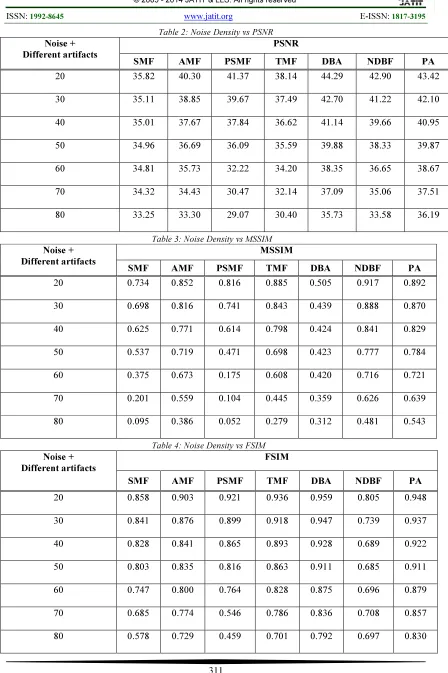
[image:6.595.89.287.231.382.2]Table 2: Noise Density vs PSNR Noise +
Different artifacts
PSNR
SMF AMF PSMF TMF DBA NDBF PA
20 35.82 40.30 41.37 38.14 44.29 42.90 43.42
30 35.11 38.85 39.67 37.49 42.70 41.22 42.10
40 35.01 37.67 37.84 36.62 41.14 39.66 40.95
50 34.96 36.69 36.09 35.59 39.88 38.33 39.87
60 34.81 35.73 32.22 34.20 38.35 36.65 38.67
70 34.32 34.43 30.47 32.14 37.09 35.06 37.51
80 33.25 33.30 29.07 30.40 35.73 33.58 36.19
Table 3: Noise Density vs MSSIM Noise +
Different artifacts
MSSIM
SMF AMF PSMF TMF DBA NDBF PA
20 0.734 0.852 0.816 0.885 0.505 0.917 0.892
30 0.698 0.816 0.741 0.843 0.439 0.888 0.870
40 0.625 0.771 0.614 0.798 0.424 0.841 0.829
50 0.537 0.719 0.471 0.698 0.423 0.777 0.784
60 0.375 0.673 0.175 0.608 0.420 0.716 0.721
70 0.201 0.559 0.104 0.445 0.359 0.626 0.639
80 0.095 0.386 0.052 0.279 0.312 0.481 0.543
Table 4: Noise Density vs FSIM Noise +
Different artifacts
FSIM
SMF AMF PSMF TMF DBA NDBF PA
20 0.858 0.903 0.921 0.936 0.959 0.805 0.948
30 0.841 0.876 0.899 0.918 0.947 0.739 0.937
40 0.828 0.841 0.865 0.893 0.928 0.689 0.922
50 0.803 0.835 0.816 0.863 0.911 0.685 0.911
60 0.747 0.800 0.764 0.828 0.875 0.696 0.879
70 0.685 0.774 0.546 0.786 0.836 0.708 0.857
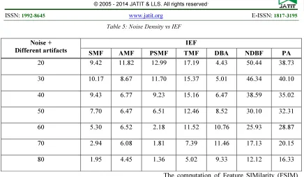
Table 5: Noise Density vs IEF
Noise + Different artifacts
IEF
SMF AMF PSMF TMF DBA NDBF PA
20 9.42 11.82 12.99 17.19 4.43 50.44 38.73
30 10.17 8.67 11.70 15.37 5.01 46.34 40.10
40 9.43 6.77 9.23 15.16 6.47 38.59 35.02
50 7.70 6.47 6.51 12.46 8.52 30.10 32.31
60 5.30 6.52 2.18 11.52 10.76 25.93 28.87
70 2.94 6.08 1.81 7.39 11.46 17.13 20.15
80 1.95 4.45 1.36 5.02 9.33 12.12 16.33
The metric for comparison are defined as follows:
PSNR 10/0110 23 (8)
MSE ∑ ∑
o r (9)
Correlation
∑ ∑ .
∑ ∑ .∑ ∑
(
10)
99:;0, < σ
σ
σ (11)
MSSIM ∑ SSIM o ,r (12)
Where oij is the original image, rij is the
reconstructed image and o> is the mean of oij,r̅ is the mean of rij, σo and σr are standard deviations
of original and restored images, oij and rij are the
image contents of qth local window and G is the
number of local windows in the image. T1 and T2
are positive constant and both values are fixed for all the images. The Structure SIMilarity (SSIM) index between the original image and reconstructed image is discussed in SSIM [22].
20 30 40 50 60 70 80 0 10 20 30 40 50 60 70 80 90 Noise Density(%) M e a n S q u a re E rr o r( M S E )
Noise Density VS MSE
SMF AMF PSMF TMF DBA NDBF PA
20 30 40 50 60 70 80
28 30 32 34 36 38 40 42 44 46 Noise Density(%) P e a k S ig n a l to N o is e R a ti o (P S N R )
Noise Density VS PSNR
SMF AMF PSMF TMF DBA NDBF PA
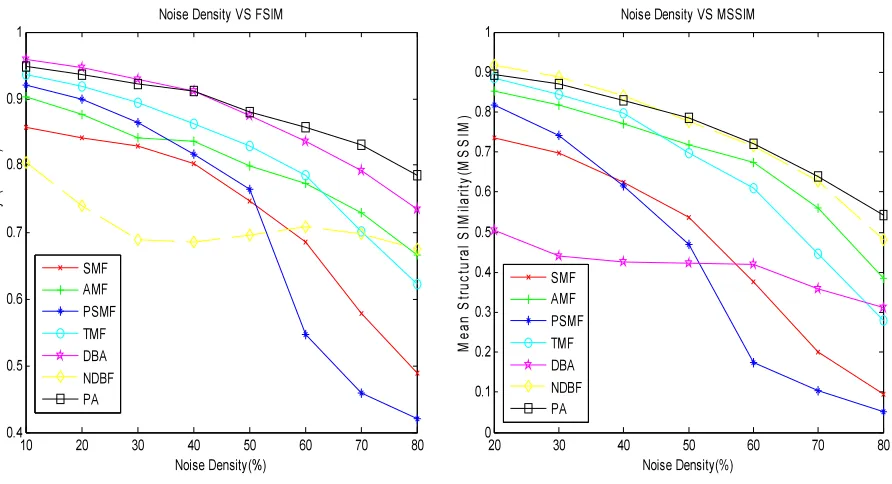
20 30 40 50 60 70 80 0 0.1 0.2 0.3 0.4 0.5 0.6 0.7 0.8 0.9 1 Noise Density(%) M e a n S tr u c tu ra l S IM il a ri ty (M S S IM )
Noise Density VS MSSIM
SMF AMF PSMF TMF DBA NDBF PA
10 20 30 40 50 60 70 80
0.4 0.5 0.6 0.7 0.8 0.9 1 Noise Density(%) F e a tu re S IM ila ri ty ( F S IM )
Noise Density VS FSIM
[image:9.595.84.517.81.395.2]SMF AMF PSMF TMF DBA NDBF PA
Fig. 4.Comparison Graphs Of MSE And PSNR At Different Noise Densities
[image:9.595.79.525.457.699.2]20 30 40 50 60 70 80 0 10 20 30 40 50 60 Noise Density(%) Im a g e E n h a n c e m e n t F a c to r( IE F )
Noise Density VS IEF
SMF AMF PSMF TMF DBA NDBF PA
20 30 40 50 60 70 80
0.1 0.2 0.3 0.4 0.5 0.6 0.7 0.8 0.9 1 Noise Density(%) C o rr e la ti o n
Noise Density VS Correlation
SMF AMF PSMF TMF DBA NDBF PA
20 30 40 50 60 70 80
-5 0 5 10 15 20 25 30 Noise Density(%) V is u a l S ig n a l-to -N o is e R a ti o ( V S N R )
Noise Density VS VSNR
SMF AMF PSMF TMF DBA NDBF PA
20 30 40 50 60 70 80
0 1 2 3 4 5 6 7 8 Noise Density(%) T im e ( S e c o n d s )
Noise Density VS Time
SMF AMF PSMF TMF DBA NDBF PA
Fig.6 Comparison Graphs Of IEF And Correlation At Different Noise Densities
Table 7: Noise Density vs VSNR
Noise + Different artifacts
VSNR
SMF AMF PSMF TMF DBA NDBF PA
20 13.58 13.63 15.68 16.11 9.23 25.57 24.24
30 13.09 11.60 13.06 14.32 7.50 22.79 21.98
40 11.62 10.08 11.02 13.02 7.49 19.12 19.88
50 8.60 9.25 6.49 11.75 7.40 17.52 18.07
60 5.25 8.21 1.50 8.47 8.08 13.39 15.48
70
1.67 6.36 -0.69 5.81 7.88 10.42 12.53
80 -0.79 5.28 -1.66 2.86 6.03 7.46 10.57
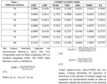
Table 8: Noise Density vs Computation Time
Noise + Different artifacts
COMPUTATION TIME
SMF AMF PSMF TMF DBA NDBF PA
20 0.0886 0.3420 0.1816 0.2109 0.6202 4.9422 0.3040
30 0.0894 0.3612 0.1972 0.2089 0.6635 6.6055 0.3025
40 0.0892 0.4012 0.2306 0.2091 0.6086 5.3661 0.3034
50 0.0889 0.4679 0.1953 0.2175 0.5983 6.0670 0.3112
60 0.0894 0.6330 0.1408 0.2251 0.6100 6.0891 0.3377
70 0.0977 0.9938 0.1532 0.2260 0.6137 7.0378 0.3539
80 0.1105 1.7512 0.1361 0.2190 0.6604 7.1847 0.3757
The Feature Similarity separates the
measurement between oij and rij into Two
Components, each for Phase congruency (PC)or
Gradient magnitude (GM). The FSIM index between oij and rij is defined as
FSIM ∑∈Ω".#$"
∑∈Ω#$"
(13)
Where, SL (x) = SPC (x) · SG (x).
S#$x #$#$".#$"
"#$
"
(14)
Sx "."
"
"
(15)
[image:11.595.77.512.411.752.2]image are visible. If the distortions are below the threshold of detection, the distorted image is considered to be of perfect visual fidelity. If the distortions are above threshold, then it operates based on the low-level visual property of perceived contrast, and the mid-level visual property of global precedence [24].VSNR is computed based on a simple linear sum of these distances.
4. CONCLUSION
An adaptive based artifacts removal algorithm for removal of strip lines, drop lines, blotches and impulse noise is developed. The proposed algorithm detects noise variance level and then proper method is selected depending upon the variance. The output of the filter is a particular value which replaces the current pixel value at that point on which the value is centered at that time. The performance of this algorithm is evaluated in terms of MSE, PSNR, MSSIM, FSIM, IEF and VSNR. The results show that the algorithm is more efficient to remove strip lines, drop lines, blotches along with impulse noise varying up to 80%. The improvement in this algorithm is that it replaces the several independent algorithms required to remove different artifacts. The proposed algorithm gives better result for low to high noise densities and preserves edges satisfactorily. It can be further improved for the application in video.
REFERENCES
[1] J.Astola and P.Kuosmanen, Fundamentals
of Nonlinear Digital Filtering, CRC Press,
New York, NY, USA, 1977.
[2] I.Pitas and A.N.Venetsanopoulos, Nonlinear
Digital Filters: Principles and Applications,
Kluwer Publishers, Boston, Mass, USA, 1990.
[3] S.M.Shahrokhy,”Visual and statistical
quality assessment and improvement of
remotely sensed images,” in Proceedings of
the 20th Congress of the International Society for Photogrammetry and Remote
Sensing (ISPRS’04), pp.1-5.Istanbul,
Turkey, July 2004.
[4] A.U.Silva and L.Corte-Real,”Removal of
blotches and line scratches from film and video sequences using a digital restoration
chain,” in Proceedings of the
IEEE-EURASIP workshop on Nonlinear Signal
and Image Processing (NSIP ‘ 99)
,pp.826-829,Antalya,Turkey,June 1999.
[5] A.Kokaram,”Detection and removal of line
scratches in degraded motion picture
sequences, “in Proceedings of the 8th
European Signal Processing Conference
(EUSIPCO’ 96), vol.1, pp.5-8, Trieste, Italy,
September 1996.
[6] H.Hwang and R.A.Haddad,”Adaptive
median filters: new algorithms and results,
“Transactions on Image Processing, vol.4,
no.4, pp.499-502, 1995.
[7] Raymond H.Chan, Chung-wa, and Mila
Nikolova.”Salt-and-pepper noise removal by median-type noise detectors and detail
preserving regularization”, IEEE
Transaction on Image Processing, vol.14,
no.10, pp.1479-1485, oct.2005.
[8] K.S.Srinivasan and D.Ebenezer,”A new fast
and efficient decision-based algorithm for
removal of high density impulse
noises,”IEEE signal processing Letters,
vol.14, no.3, pp.189-192, March 2007.
[9] S.Manikandan and D.Ebenezer,”A
Nonlinear decision-based algorithm for removal of strip lines, drop lines, blotches, band missing and impulses in images and
videos,” in proceedings of EURASIP
Journal on Image and Video Processing,
Article ID 485921, 2008.
[10] V.Jayaraj, D.Ebenezer and
K.Aiswarya,”High density salt and pepper noise removal in images using improved
adaptive statistics estimation filter “in
proceeding of International Journal on
Computer Science and Network Security,
vol.9, no.11, pp.170-176.
[11] H. C. Reeves and J. S. Lim,
“Reduction of blocky effect coding,” Opt.
[12] C. J. Crouse and M. R. Kannan, “Simple algorithm for removing blocking artifacts in block-transform coded images,” IEEE Signal Processing Letter, vol. 5, pp. 33-35, Feb. 1998.
[13] F. Zhigang and L. Fu, “Reducing
artifacts in JPEG decompression by
segmentation and smoothing,” in Int. Conf.
Image Processing ’96, vol. 2, Sept. 1996,
pp. 17-20.
[14] L. Yung-Kai, L. Jin, and C.-C. J.
Kuo, “Image enhancement for low-bit-rate
JPEG and MPEG coding via post
processing,” Proc. SPIE, vol. 2727, no. 3,
pp. 1484-1494, Mar. 1996.
[15] R. A. Gopinath, H. Guo, M. Lang, and
J. E. Odegard, “Wavelet-based post-processing of low bit rate transform coded,”
in Proc. IEEE Int. Conf. Image Processing,
1994, pp. 913-917.
[16] D. L. Donho, “De-noising by soft
thresholding,” IEEE Trans. Inform. Theory,
vol. 41, pp. 613–627, May 1995.
[17] Z. Xiong, M. T. Orchard, and Y.
Zhang, “A deblocking algorithm for JPEG compressed images using over complete
wavelet representations,” IEEE Trans.
Circuits Syst. Video Technol., vol. 7, pp.
433-437, 1997.
[18] Gonzalez and woods, “Digital image
processing”, Prentice hall, 2nd Edition,
2001.
[19] Wang.Z and Zhang.D,”Progressive
Switching Median Filter for removal of
impulse noise for highly corrupted
Images,”IEEE Transaction Circuits and
Systems, vol.46, no.1, pp.78-80.
[20] Jiang Bo, Huang Wei. “Adaptive
threshold median filter for multiple-impulse
noise,” Journal of Electronic Science and
Technology of China, vol. 5 no.1, pp. 70-74,
2007.
[21] P.Tamilselvam, M.V.Mahesh and
G.Prabhu,”Blotches and impulse removal in colour scale images using non-linear
decision based algorithm,” International
journal of scientific research publications,
vol.3, no.4, pp.1-5, 2013.
[22] Z. Wang, A. C. Bovik, H. R. Sheikh,
and E. P. Simoncelli, "Image quality
assessment: From error visibility to
structural similarity,"IEEE Transactions on
Image Processing, vol. 13, no. 4, pp.
600-612,Apr. 2004.
[23] Lin Zhang, Lei Zhang, Xuanqin Mou,
and David Zhang,"FSIM: a feature
similarity index for image quality
assessment", IEEE Transactions on Image
Processing, vol. 20, no. 8, pp. 2378-2386,
2011.
[24] D. M. Chandler and S. S. Hemami,”
VSNR: A Wavelet-Based Visual
Signal-to-Noise Ratio for Natural Images,”IEEE
Transactions on Image
Processing, Vol. 16 (9), pp.