PARIS RESEARCH LABORATORY
d i g i t a l
March 1992 Fran¸cois Bourdoncle
Abstract Interpretation by
Dynamic Partitioning
Fran¸cois Bourdoncle
This paper has also been published in the Journal of Functional Programming.
c
Digital Equipment Corporation 1992
The essential part of abstract interpretation is to build a machine-representable abstract domain expressing interesting properties about the possible states reached by a program at run-time. Many techniques have been developed which assume that one knows in advance the class of properties that are of interest. There are cases however when there are no a priori indications about the “best” abstract properties to use. We introduce a new framework that enables non-unique representations of abstract program properties to be used, and expose a method, called dynamic partitioning, that allows the dynamic determination of interesting abstract domains using data structures built over simpler domains. Finally, we show how dynamic partitioning can be used to compute non-trivial approximations of functions over infinite domains and give an application to the computation of minimal function graphs.
R ´esum ´e
2 Widening operators 2
3 Representations 5
4 Dynamic partitioning 9
4.1 Basic partitioning : : : : : : : : : : : : : : : : : : : : : : : : : : : : : 9 4.2 Basic functional partitioning : : : : : : : : : : : : : : : : : : : : : : : : 12 4.3 Functional partitioning : : : : : : : : : : : : : : : : : : : : : : : : : : : 16
5 Applications 22
5.1 Multi-intervals : : : : : : : : : : : : : : : : : : : : : : : : : : : : : : : 22 5.2 Minimal function graphs : : : : : : : : : : : : : : : : : : : : : : : : : : 23
6 Conclusion 28
1 Introduction
Abstract interpretation, as defined in Cousot [2, 4, 6], provides a general framework aimed at computing invariance properties of programs. These properties describe the run-time states that can be reached from a set of initial states P
0 by means of a transition function over the subsets of the set of run-time statesS, which defines the operational semantics of a given program. When is continuous over the lattice (P(S);), the invariant I=
S n2N
n
(P 0) is also the least fixed point lfp(Φ) of the functionΦ=P :(P
0
[ (P)). In most cases however, S is infinite, and methods must be developed to determine a safe and finitely represented approximation of this least fixed point. Patrick and Radhia Cousot introduced the notion of Galois connection (;) as a general tool for building such approximate frameworks. The
abstraction functionmaps a set of statesP to an elementP
#of a finitely represented abstract
(approximate) lattice (P#(S);v) whereas the concretization functionmaps an abstract state
P
#to a set of states, called its meaning. Then, by defining a safe approximationΦ#ofΦ, i.e.,
a function such thatΦ#wΦ, one can determine an approximate invariant I
#
=lfp(Φ
#)
which is a safe approximation of I, i.e.,(I
#)
I.
However, when the approximate lattice is of infinite height, the iterative computation of the approximate invariant may not finitely converge, and speedup techniques, such as widening and narrowing, must be used to determine a safe approximation of I#. But in many cases, there is not even a clear indication about how to build a good and finitely represented abstract lattice. This happens when there is no indication about what the least fixed point will “look like”, and therefore no advance knowledge of the properties that should be expressed in the abstract lattice P#(S) to precisely describe the invariant I. Differently stated, there is a gap between the exact lattice P(S) and the abstract lattices that one can a priori build or think about. This is true in particular when functions over infinite domains are approximated. Moreover, most implementations of abstract interpretation have to deal with the problem of testing the equivalence of the data structures used to represent lattice elements (i.e., testing the equality of their meaning). This test is often very costly and difficult to implement, as with the abstract interpretation of functional or logic programs for instance, and it would be desirable to design a framework that avoids such a test.
The aim of this paper is to discuss a technique, which we call dynamic partitioning, that can be used to compute non-trivial, safe approximations of program invariants in the above cases, by dynamically selecting interesting and finitely represented abstract properties without having to test the equality of their meaning.
practical applications and show how dynamic partitioning can be used to effectively compute non-trivial, safe approximations of minimal function graphs.
2 Widening operators
The Galois connection approach described above is perfectly adequate when the abstract lattice P#(S) is of finite height, since the iterative computation of the least fixed point ofΦ
#
over P#(S) will necessarily converge in a finite amount of time. However, some interesting program properties, such as the range of integer variables, are expressed in a lattice of infinite height. Even if the integer variables were bounded, choosing for instance Z=f! ;. . .;!
+
g, ! = 2
w 1 ,!
+
=2 w 1
1, the interval lattice I(Z) is still of height2 w
, and fixed point computations may in theory require up to the same number of iterations. A speedup technique has been proposed in Cousot [2] that uses so called widening operators to transform infinite iterative computations into finite but approximated ones. So let us suppose for instance that one has a program functionLoopdefined in ML as follows:
fun Loop i = if i < 100 then Loop (i + 1) else
i
Suppose now that one wants to compute the values returned byLoopfor a set of input data
specifications. Loop being recursive, this computation may require computing the value returned byLoopfor arguments that were not present in the initial data set. Therefore, the goal of an interprocedural abstract interpretation framework will be to determine this minimal
function graph describing the minimal information aboutLoopneeded to compute its value for every argument in the original specification. This notion of minimal function graph was first introduced in Jones and Mycroft [10], but was in essence already present in Cousot [5]. A program stateha;bi2 ZZ
? therefore consists of an input value
aand a return value b=Loop(a), where the special value?denotes nontermination. Generalizing the idea used by Jones and Mycroft for constant propagation, we can approximate the minimal function graph ofLoopby a pair of intervals representing an approximation of all ofLoop’s arguments and all ofLoop’s results. This approximate minimal function graph is therefore the least fixed pointX
#of the monotonic functionΦ#over the lattice I(Z)
I(Z) defined as follows:
Φ#
hi;vi = hi 0
;?i_hΦ
#
1( i);Φ
#
2( i;v)i wherei
0is the input data specification, and the two functionsΦ
#
1andΦ
#
2are defined by:
Φ#
1(
i) = incr
#(
i^[! ;99])
Φ#
2(
i;v) = v_(i^[100;!
+])
where the strict abstract function incr#is defined by:
incr#(?) = ?
incr#[a;b] = [min(a+1;!
+)
;min(b+1;!
The least fixed pointX
#is known to be the upper limit of the increasing chain:
( X
#
0
= h?;?i X
#
n+1
= Φ
#(
X
#
n)
But this limit can take a very long time to compute. For instance, ifi 0
=[0;0], this least fixed point is equal toh[0;100];[100;100]iand is reached after 102 iterations. One must therefore find a way to speedup this computation in order for it to be tractable. To this end, we introduce the widening operatorrIover I(Z), taken from Cousot [2] p. 247, or [6] p. 334:
?rIx = xrI ? = x [a
1 ;b
1]
rI [a 2
;b 2]
= [ifa 2
<a 1then
! elsea 1 ; if b 2 >b 1then ! +else b 1]
This non-commutative operator generalizes “unstable” bounds of its right argument. It is a safe approximation of the join operator, and is such that for every increasing chain (x
n) n2N, the increasing chain (y
n)
n2Ndefined by: ( y 0 = x 0 y
n+1
= y n
rIx n+1 is always eventually stable, i.e., there exists an
0 such that:
8n n 0 :
y n
= y n
0. Under these assumptions, it is well known ([6], theorem 10-30, p. 334) that the upper limitY
#of the
increasing chain: 8 > < > : Y # 0
= h?;?i Y
#
n+1
= Y
#
n rIΦ
#(
Y
#
n) if :(Φ
#( Y # n) Y # n) Y #
n+1
= Y
#
n if Φ
#( Y # n) Y # n
where the widening operator is applied componentwise, is a post fixed point of Φ#, i.e., Φ#(
Y
#)
Y
#, and, therefore, is a safe approximation of
X
#, i.e.,
X
#
Y
#. Note that since
here:
yx =) xrIy=x this chain could be simply defined by:
( Y
#
0
= h?;?i Y
#
n+1
= Y
#
n rIΦ
#(
Y
#
n) So for example, with input data specification i
0
= [0;0], one can compute the increasing chain:
Y
#
0
= h?;?i Y
#
1
= h[0;0];?i Y
#
2
= h[0;!
+] ;?i Y # 3 = Y #
= h[0;!
+]
;[100;!
+]
i whose limitY
#is a safe approximation of the least fixed point:
X
#
This result could also be improved by using the narrowing operator∆Idefined by:
?∆Ix = x∆I? = ? [a
1 ;b
1] ∆I [ a
2 ;b
2]
= [ifa 1
=! thena
2else min( a
1 ;a
2) ;
ifb 1
=!
+then
b
2else max( b
1 ;b
2)]
This operator satisfies the canonical condition:
8x;y2I(Z) : xy =) x x∆I y y and is such that for every decreasing chain (y
n)n2N, the chain ( z
n)n2Ndefined by: (
z 0
= y 0 z
n+1
= z n∆I
y n+1
is always eventually stable. It is known that the lower limitZ
#of the decreasing chain:
( Z
#
0
= Y
#
Z
#
n+1
= Z
#
n∆IΦ
#(
Z
#
n)
starting from the post fixed pointY
#, is a safe approximation of
X
#. On our example, this
gives, after only 2 iterations:
Z
#
0
= h[0;!
+]
;[100;!
+]
i Z
#
1
= Z
#
= h[0;100];[100;!
+]
i
This example shows how good results can be obtained by using very na¨ıve and “brute force” widening and narrowing operators. Of course, it might be argued that the interval [0;100] inferred by the computation could have been easily determined by simply looking at the text of the program, and that a finite abstract lattice could thus have been built a priori. We shall see, in section 5.2, an example that shows that this is not always the case, and in practice, building ad-hoc approximate functional lattices is simply not feasible. However, since we already know how to deal with intervals, it is very tempting to describe minimal function graphs by sets of interval pairs, instead of a single pair of intervals. The advantage of such a representation is that it is very flexible, and does not establish in advance any particular tradeoff between complexity and precision.
3 Representations
Definition 1 Let (D ;?;v) be a countable complete partial order (cpo), R a set, and
:R!Da meaning function. Then (R;;;r) is said to be a representation ofDif:
i) (R;?;) is a partial order
ii) The meaning functionis monotonic
iii) Each elementd2Dcan be safely abstracted by an element(d)2R, i.e.:
((d)) w d
iv) Each binary operatorr i:
RR!Rof the sequencer=(r i)
i2Nis such that:
8r;r 0
2R: (
r rr
i r
0
(r 0
) v (rr i r
0 )
v) For everyfr i
g i2N
R, the chain (r 0 i
)i2Ndefined by:
( r
0 0
= r 0 r
0 i+1
= r 0 i
r i r
i+1
has an upper bound.
A representation is said to be complete if (R;) is a cpo, finite if every element ofRhas a
finite encoding, and tractable if the chain (r 0 i)
i2Nis always eventually stable.
This definition has some similarities with the definition of the upper approximation (D
#
;) of a complete lattice (D ;v) using a Galois connection, i.e., a pair of monotonic functions (;),
:D!D
#and
:D
#
!Dsuch that:
8(d;d
#)
2DD
# :
(d)d
#
() dv(d
#)
The difference between the two definitions is that our framework makes very weak assumptions aboutR and D and generalizes the case where R and D are both complete lattices, since we only require that be safe. As a matter of fact, is not even needed in the framework, and only the existence of a safe approximation for every concrete element is required. This allows in particular different representations to have the same meaning and one can choose arbitrarily between them, hence the term representation. Therefore, the traditional inequality
Id
R, which becomes an equality when
is one-to-one, does not hold in this framework.
Each elementary widening operator r
i of the widening operator
r = (r i)
i2N is an alternative to a join operator over the abstract latticeD
#which does not necessarily exist if
R is a partial order. The conditions imposed onr
overRcan be built from increasing chains over D, as we shall see below. WhenRand D are both complete lattices, the operatorr of a tractable representation is a straightforward generalization of the classical widening operator, in the sense that(rr
i r
0
)w(r)t(r 0
) and every increasing chain built usingris eventually stable.
Another remark concerning this framework is that condition (v) is trivially satisfied for any complete representation, for every increasing chain has a least upper bound. Differently stated, the widening operatorris not necessary in a complete representation to prove the existence of a least upper approximation. But even so, it can be very interesting to have such a widening operator to define finite and tractable frameworks, as we have seen in section 2. Also, note that the use of widening operators over non-complete lattices was already present in Cousot and Halbwachs [3], where the lattice of finitely represented convex hulls is not complete.
Finally, it should be noted that our framework can be very easily generalized to cases where (R;) is only a preorder
1
, in which case the meaning function need not be monotonic and the conditions imposed on the elementary widening operators must be:
8r;r 0
2R : (
(r) v (rr i r
0 )
(r 0
) v (rr i r
0 )
Preorders have been used for instance in Stransky [12]. However, the problem with such very general frameworks is that not much can be said about them, for they are essentially defined by the properties of the widening operator r. Moreover, preorders are not very easy to work with, for representations having the same meaning can “oscillate” during the computation and one must be able to finitely compute the equivalence of representations (i.e.,
(r)=(r 0
)) to detect the stabilization of increasing chains. As we noted earlier, this is not necessary here since stabilization is detected by the equality of representations (i.e.,r=r
0 ). Hence, our framework is perfectly suited to cases whereRis implemented using very complex
data structures for which the equivalence test is intractable or very costly, since we require that equivalent representations be comparable only when they are “similar enough”. It is
interesting to note that a comparable idea, which was only a heuristic at the time, was used in the design of the widening operator of Cousot and Halbwachs [3] which preserves as much as possible the representations of convex hulls during iterative computations.
So let (R;;;r) be a representation ofD, and Φ2 D! Dbe a continuous function, that is, a monotonic function such that for every directed subsetC D: Φ(
F C)=
F
Φ(C). It is well known that the least fixed point ofΦis:
= lfp(Φ) = G
i2N
Φi (?)
If the elements ofD do not have a finite encoding, it may be impossible to compute this increasing chain. So let us suppose that one can define a safe approximationΦ#ofΦoperating over the set of (supposedly finitely encoded) representationsR, that is, a function Φ
# such
that:
Φ
#
w Φ
1
One can choose in particular2
any functionΦ#such thatΦ#
Φ, for by monotonicity ofand property (iii):
Φ
#
w ()Φ w Φ
but this is not mandatory. The only thing we really need is any safe approximation ofΦ. Our problem is now: how can we compute a safe representation ofusingΦ
#which is the only
function that we can possibly compute? To this end, let us define the chain (r i)
i2Nby: (
r 0
= ? r
i+1
= r i r iΦ #( r i)
Theorem 2 The chain (r i)
i2N is an increasing chain over
R that has an upper bound r !
which is a safe representation of the least fixed point ofΦ, that is:
(r !)
w
Proof. Let us first define the increasing chain ( i)
i2Nby
0
=?and i+1
=Φ( i). It is clear that(r
0)
w?=
0. Suppose by induction that (r
i) w
i. Then by definition of the widening operatorr:
(r i+1)
= (r i r iΦ #( r i))
w (Φ
#(
r i))
ButΦ#being a safe approximation ofΦ, and by monotonicity ofΦ:
(Φ
#(
r i))
w Φ((r i))
w Φ( i)
=
i+1
which proves that eachr
iis a safe approximation of
i. But thanks to the first property of r,r
i+1 r
i, and ( r
i)
i2Nis an increasing chain which has an upper bound r
!. Finally, by monotonicity of: 8i:
i v(r
i) v(r
!), which implies that
v(r !).
Using a finite and tractable representation, one can therefore compute a non-trivial, safe and finitely represented approximation of the least fixed pointof any continuous functionΦover
D, even if the representationRdoes not have a maximum element (which would be of course a trivial safe approximation of any element ofD).
However, as in section 2, it is possible to compute an even better representation r 0 ! of the least fixed point of Φ by defining a narrowing operator ∆ = (∆
i)i2N such that every elementary narrowing operator∆isatisfies:
8r;r 0
2R; 82D : v(r); (r 0 ) =) ( r∆ i r 0 r v(r∆
i r
0 )
2
and computing the lower limit of the decreasing chain (r 0 i)
i2Ndefined as follows: ( r 0 0 = r ! r 0 i+1
= r 0 i∆ i Φ #( r 0 i)
Note that, once again, the first condition imposed on∆i enforces the chain condition whereas the second condition enforces the safeness of the computation, that is, this condition ensures that the narrowing operator will not “jump below” the least fixed point, as shown by the following theorem.
Theorem 3 When the decreasing chain (r 0 i)
i2Nis eventually stable, its lower limit is a safe
representation of the least fixed point ofΦ.
Proof. We first note thatr 0 0
=r
!being a safe representation of
, we have:
(r 0 0)
w
Now, suppose by induction that:
(r 0 i)
w
then obviously, by monotonicity ofΦ:
(Φ
#(
r 0 i))
w Φ((r 0 i))
w Φ() =
and therefore:
(r 0 i+1)
= (r 0 i∆ i Φ #( r 0 i)) w
which shows that the lower limitr 0 !
=r 0 i0
for somei 0
2N is a safe representation of.
Note that, contrary to the classical widening/narrowing approach, we do not require that the meaning of the first elementr
0 0
=r
! be a post fixed point ofΦ, which, consequently, avoids comparing(r
i) withΦ( (r
i)) at each stage of the iterative computation of r
!, as in section 2. This property is very important if, as stated in the introduction, comparing the meaning of representations is very costly. However, if the elementary widening operatorr
i satisfies the natural stability condition:
8r;r 0
2R : (r 0
) v (r) =) rr i
r 0
= r
as does the widening operatorrIover the interval lattice I(Z), then(r
!) will always be a post fixed point ofΦ. Elementary widening operators satisfying this condition will be called stable. Note that complex widening operators, such as the ones that will be presented in the following sections, will not generally be stable. Intuitively, since we require that two representations
randr 0
be comparable only when they are “similar enough”, the stability test(r 0
) v(r) will be approximated, and, therefore, redundant informationr
0
added to a representationrwill sometimes lead to a loss of precision.
4 Dynamic partitioning
The aim of this section is to build generic representations based on the idea of “non-redundancy”. We shall first talk about what we call basic partitioning, which is a technique that can be used to build representations of a concrete complete lattice (L;?;>;v;t;u) using well chosen subsets ofAwhenAis an upper approximation ofL. We shall then discuss two other methods, called basic functional partitioning and functional partitioning used to build representations of functionsF :C !B over an infinite setC, using subsets ofAB when
Ais an upper approximation of P(C) andB is a lattice. We start by defining two notions of non-redundancy for the subsets of a latticeA.
Definition 4 A subsetP of a latticeA is said to be non-redundant if it does not contain?
and:
8a;a 0
2P : aa 0
=) a=a 0
P is said to be strongly non-redundant if it does not contain?and:
8a;a 0
2P : a6=a 0
=) a^a 0
=?
Non-redundant subsets are often called crowns or antichains. The set of non-redundant and strongly non-redundant subsets of A will be noted respectively Pnr(A) and Psnr(A). Two elements of a non-redundant subset are either equal or not comparable, whereas they are equal or have “nothing in common” if they belong to the same strongly non-redundant subset. Note that strong non-redundancy implies non-redundancy.
4.1 Basic partitioning
So let us suppose thatAis an upper approximation of a complete lattice Land let (;) denote the Galois connection between the two lattices. We wish to build a representation ofL using the subsets ofA. The most natural meaning of a subsetP ofAis of course:
Γ(P) = G
a2P (a)
that is, the least upper bound of the set of concrete elements denoted by the abstract elements ofP. Let us define the binary relationover P(A) by:
P P 0
() 8a2P ; 9a 0
2P 0
: aa 0
This relation is similar to the preorder used to build the lower powerdomain (see Gunter and Scott [8] p. 653), sometimes called the Hoare powerdomain, or the relational powerdomain (see Schmidt [14], p. 295). The originality of our framework is that using well chosen subsets of P(A), we can turn this preorder into a partial order and avoid using principal ideals and complex power domains, as in Mycroft and Nielson [11] for instance.
Proof. is obviously a preorder. So letP P 0
,P 0
P, anda2P. Then there exists a 0 2 P 0 and a 00
2 P such that: a a 0
a 00
, and by non-redundancy: a = a 00
, which implies that: a=a
0 2P
0
, and henceP P 0
. But similarlyP 0
P, and thusis a partial order. Finally, it is easy to show that the monotonicity ofimplies the monotonicity ofΓ.
Under more restrictive conditions, we can show that (Psnr(A);) is a complete partial order.
Theorem 6 IfAis meet-continuous 3
, then (Psnr(A);) is a cpo.
Proof. To show that (Psnr(A);) is complete, let (P i)
i2Nbe an increasing chain. Using the diagonal argument and the definition of, one can build a (possibly infinite) set of increasing chainsfC
j g
j2J,
J N,C j
=(c ji)
i2N, such that for all
i2N :P i
=fc ji
g j2J
f?g. But Abeing a complete lattice, each increasing chainC
j has a limit l
j
2A. The only possible candidate to the upper limit of the chain (P
i)
i2Nis therefore fl
j g
j2J. But then for all j 6=j
0 : l j ^l j 0 = W C j ^ W C j 0 = W i ( c ji ^ W C j 0) = W i;i 0 ( c ji ^c j 0 i 0) = W i;i
0 ? = ?
which shows that fl j
g
j2J is strongly non-redundant and is the least upper bound of the chain (P
i) i2N.
Under the light of this theorem, one might think that it is a good idea to limit oneself to the strongly non-redundant subsets of A, since they form a complete partial order, and appear to be “less arbitrary” than the general non-redundant subsets ofA. But it depends a lot on the “shape” of the abstract latticeA. Intuitively, for strongly non-redundant subsets to be useful, every abstract elementa2Ashould be the least upper bound of a set of atoms. This can be formalized by saying that A should be an algebraic atomic lattice with a strongly non-redundant basisAof atoms such that:
8a2A : a= _
(A\#a)
where# a =fa 0
2A : a 0
agis the principal ideal generated bya. Standard examples of such lattices are (P(S);) and the interval lattice I(Z), with bases ffsgg
s2S and
f[i;i]g i2Z respectively. Counter-examples are complete total orders, for which every subset with more than two elements is necessarily redundant. More generally, one can prove the following theorem.
3
A complete latticeLis meet-continuous (see Gierz [7] p. 30) if for every directed subsetDLand every
elementx2L:x^
W D=
W
Theorem 7 Let (A;?;>;;_;^) be an upper approximation of P(S), such thatis
one-to-one,(?)=;, and:
[s]6=[s 0
] =) [s]^[s 0
]=? (where [s]=(fsg))
ThenAis an algebraic atomic lattice,A =f[s] : s2 Sgis a strongly non-redundant basis
ofA, andf(a) : a2 Agis a partition of S. Moreover, if is _-continuous, thenA is
meet-continuous.
Proof. We first note that being one-to-one, =Id A,
is ^-continuous and is [-continuous (Cousot [4], theorem 4.2.7.0.3, p. 4.33). Suppose now that there existss2S such that [s] = ?. Then [s] = (fsg) ? and by definition of Galois connections,
fsg(?)=;which is impossible. ThusAis strongly non-redundant. But:
x2A\#a () 9s2S : x=(fsg) a () 9s2S : x=[s]^fsg(a) () 9s2(a) : x=[s]
ThereforeA\#a=(a) =f[s] : s2(a)g. In order to show thata= W
(a), we shall first show that(a)=
S a2(a)
(a). ButId
P(S)and thus: S
a2(a)
(a) = S
s2(a)(
)(fsg)
S
s2(a)
fsg = (a)
Conversely, letx 2 S
s2(a)
([s]). Then there existsfsg(a) such that fxg([s]), and hence by monotonicity of:
(fxg) [s] = (fsg) ((a)) = a
which implies thatfxg(a), that is,x2(a). Therefore:
a = ()(a) = ( S
a2(a) (a)) =
W a2(a)(
)(a) = W
(a)
Now, whenis_-continuous, then for everya2Aand every subsetX A:
(a^ W
X) = (a)\ S
f(x) :x2Xg =
S
f(a)\(x) :x2Xg =
S
f(a^x) :x2Xg and therefore,being[-continuous:
a^ W
X = ()(a^ W
X) =
W
f()(a^x) :x2Xg =
W
fa^x:x2Xg
which shows thatA is meet-continuous. Finally,([s]) 6=([s 0
]) implies that [s] 6=[s 0
], andbeing^-continuous,([s])\([s
0
])=([s]^[s 0
])=(?)=;, which proves that
What we need now in order to complete our framework is to define elementary widening operatorsrsuch that: P P rP
0
andΓ(P 0
)vΓ(PrP 0
). There are of course many ways to define these operators. When working with Pnr(A), the most precise widening operator can be defined by:
P rP 0
= (P [P 0
) fa 0
2P 0
; 9a2P : a 0
<ag
In fact, this widening operator behaves rather like a join operator. More generally, at each step of the computation, one can choose (either deterministically or not) a subsetP
0 of the current invariantP to coalesce. The idea of such a generalization is to replaceP by:
P [fa 0
g
fa2P : a<a 0
g
wherea
0is any element greater than W
P
0. Of course, one might choose to define a very poor widening, which does not improve the expressible properties of the framework, by:
P rP 0
= n
_ (P [P
0 )
o
It is easy to see that these definitions turn Pnr(A) into a representation framework abstracting the latticeLwhenever the “generalizations” are properly used. It is difficult to say more about these generalizations since widening operators are well known to be highly lattice-dependent. When working with Psnr(A), widening operators are even more difficult to define in the general case, and we shall only develop an example in section 5.1. Note that in practice, one will always work with the set of finite strongly non-redundant subsets ofAwhich is generally not a cpo, so the completeness of Psnr(A) will not help. Finally, note that the definition of the widening operator has a great influence over the quality of the result of the computation, as we shall see in section 5.2. Therefore, the general idea one should follow in the definition of a widening operator (r
i)
i2Nshould be to use very precise elementary operators (i.e., join-like) at the beginning of an iteration sequence, and to generalize only after these operators have precisely defined the “shape” of the least fixed point. However, as we shall see in section 5.2, there are also cases where it can be a good idea to alternate join-like operators and generalizations.
4.2 Basic functional partitioning
A central problem in abstract interpretation is to find a safe approximation of a least fixed pointF that belongs to a functional latticeC!B, where (B;?;>;v;t;u) is itself a lattice. For instance, for very simple, non-recursive programming languages,C is usually the finite set of lexical control points, andB the powerset of run-time memory states. But for more complicated, recursive languages, a control point is more naturally defined as a subpart of the run-time stack, andC is infinite. More generally, there are cases where it can be interesting to consider that control points are indeed execution traces and not only static control points. Finally, in the minimal function graph approach,C is the set of admissible inputs of program functions, andB is the lattice of possible outputs, the bottom value ofBbeing used to denote nontermination. In this paper, we shall refer to the elements of the possibly infinite setC as
Very often however, there is no need to know the value ofF for every control point, and it is sufficient to determine a safe approximationF
i w
F
fF(c) :c 2C i
g, of the values taken byF over each subset of a given partitionfC
i g
i2I of
C. This partition can be defined in a very natural way by assigning a token to each control point. This method has been proposed for instance in Sharir and Pnueli [13] and Jones [9], where tokens are used to group execution traces and coalesce the memory states associated with them.
If the set of tokens is finite, then the framework is said to be partitioned (see Cousot [6] p. 315) and the problem is equivalent to the resolution of a finite system of semantic equations. This is the case for instance in Bourdoncle [1], where a token is assigned to each run-time stack. These tokens model the “shape” of the stack (pointers, control stack. . . ) and generalize the tokens used in Sharir and Pnueli [13] that only took into account the control part of the run-time stacks.
However, if the set of tokens is infinite (or very large) and one has no idea of a good way of defining a finite partition, then the original problem of finding a safe and finitely represented approximation ofF remains to be solved. The idea is then to “lift”F so that it operates on sets of control points, and to dynamically calculate a partition ofC, instead of it being “hard wired”.
We are going to study two general methods for doing this dynamic partitioning. For each of these methods, we suppose that there is a basic (and supposedly not satisfactory) way of finitely representing sets of control points, and we intend to build a representation from this initial approximation. We shall therefore suppose that (A;?;>;;_;^) is an upper approximation of (P(C);;;C ;;[;\), and call (;) the Galois connection between the two lattices. We shall also suppose that is one-to-one and that(?) =;, which implies that is^-continuous. The elements ofA will be called abstract control points and the elements ofT =f[c] : c2Cg, where [c] =(fcg), will be called the tokens. Theorem 7 shows that wheneverT is strongly non-redundant, thenAis an algebraic atomic lattice, andT defines a partition ofC, but this hypothesis will not be necessary. Our definition therefore generalizes the classical notion of token. Finally, the elements ofBwill be called abstract values.
The first representation that we shall define is based on the very na¨ıve observation that every abstract control pointa2A implicitly defines a (possibly infinite) set of control points(a) that we shall informally call a “region”. Therefore, an easy way to approximate a function fromCintoB is to “cover” the region over which this function is different from?by a finite subset ofA, and to associate an abstract valuebwith each elementaof this subset.
If the regions of such a representationP AB do not overlap, the natural meaning of
study, in the next section, a different and non standard meaning of overlapping representations that is better suited to generalization.
Definition 8 A subsetP ofABis said to be normalized if:
8ha;bi2P ; 8ha 0
;b 0
i2P : a=a 0
=) b=b 0
For every normalized subsetP, anda;a 1
;a 2
2A, we define:
A(P) = fa2A:9b2B :ha;bi2Pg C(P) =
S
f(a) :ha;bi2Pg P(a) =
F
fb2B :ha;bi2Pg P
\ (a
1 ;a
2)
= fb:ha;bi2P ^ a 1
aa 2
g
The setA(P) is called the domain ofP, and the abstract value P(a) is the image ofabyP. The setC(P) is the concrete domain ofP, i.e., the “region” ofC covered by the domain of
P. For a normalized subsetP ofAB, the imageP(a) of every element of the domain of P is the unique elementbsuch thatha;bi2P. We call P(A;B) the set of normalized subsets P whose domains do not contain ?, and Pnr(A;B) (resp. Psnr(A;B)) the set of normalized subsets which have a non-redundant (resp. strongly non-redundant) domain. Obviously:
Psnr(A;B) Pnr(A;B) P(A;B)
We then define the meaningΓ(P) of a representationP 2P(A;B) by:
Γ(P)(c) = M P[
c]
where the monotonic functionM P :
A!Bis defined by:
M P(
x) = G
a2A(P) a^x6=?
P(a)
WhenT is a strongly non-redundant basis ofA, we obviously have:
8 2T; 8a2A : a^ 6=? () a
and therefore:
Γ(P)(c) = G
fb:ha;bi2P ^ [c]ag
which states that each control pointcis mapped to the union of the abstract valuesbattached to the elements ofA(P) by which its token [c] is “covered”, or to?if its token is not covered. Note that ifA(P) is strongly non-redundant, then an element of the basis is at most covered by a single element inA(P). It is worth mentioning at this stage that although any set of tokens can be chosen, it seems reasonable to impose thatT be strongly non-redundant. To see the problem, let us chose C = Z, A = Z
?, and [
c] =c. Then (c) = f! ;. . .;cg, the lattice (A;?;!
+
;;max;min) is totally ordered, and:
8a;a 0
2A:a6=? ^ a 0
6=? () a^a 0
which shows thatΓ(P) is constant overCand:
Γ(P)(c) = G
fb:ha;bi2Pg
Intuitively, all the “regions” defined by the abstract control points overlap, and therefore, there is no way to distinguish between the different abstract valuesb2Bof the representation. We are now going to show that Pnr(A;B) and Psnr(A;B) can be turned into partial orders.
Theorem 9 Pnr(A;B) and Psnr(A;B) are partial orders for the binary relation:
P P 0
() 8ha;bi2P ; 9ha 0
;b 0
i2P 0
: aa 0
^ bvb 0
and the meaning functionΓis monotonic over Pnr(A;B) and Psnr(A;B).
The proof is straightforward. Note that every functionF inC ! B can always be finitely abstracted byfh>;>ig and, when T is non-redundant, it can also be safely abstracted by
fh[c];F(c)i : c 2 Cg. Therefore, defining a widening operator over Pnr(A;B) will turn
Pnr(A;B) into a representation ofC !B. Elementary widening operators can be defined as follows:
We first define the domain ofPrP 0
by:
A(PrP 0
) = A(P)r b
A(P 0
)
wherer
b is any basic partitioning widening operator defined in section 4.1.
Then, for everyain the domain ofPrP 0
, we define the image ofaby:
(PrP 0
)(a) = b
whereb2Bis any abstract value such that:
b w M P(
a)tM P
0( a)
To prove thatP PrP 0
, we remark that by definitionA(P)A(PrP 0
), and therefore:
8ha;bi2P ; 9a 0
2A(PrP 0
) : aa 0
hence:
b = P(a) v M P(
a) v M P(
a 0
) v M P(
a 0
)tM P
0( a
0
) v (PrP 0 )(a 0 ) and thus: 9ha 0 ;b 0
i2PrP 0
: aa 0
^ bvb 0
Let us now prove that Γ(P 0
) v Γ(P rP 0
). So let ha 0
;b 0
i 2 P 0
and x 2 A be such that
x^a 0
6=?. By construction, we have:
C(P 0
) = [
a2A(P 0
)
(a)
[
a2A(PrP 0
)
(a) = C(P rP 0
and therefore, there exists a pairha;bi2P rP 0
such thata^x^a 0
6=?, otherwise,being ^-continuous:
(x^a 0
) = (x^a 0
) \ (a 0
)
(x^a 0
) \ S
a2A(P 0
)(a)
S
a2A(PrP 0)(
(x^a 0
) \ (a))
S
a2A(PrP 0
)(a^x^a 0
) = ;
and thus,being one-to-one, x^a 0
=?, which is absurd. Consequently,a^a 0
6=?, and therefore:
b w M P(
a)tM P
0(
a) w M P
0( a^a
0
) w b 0
which shows that:
M P
0( x) =
G ha 0 ;b 0 i2P 0 x^a 0 6=? (b 0 ) v G
ha;bi2PrP 0 x^a6=?
(b) = M PrP
0( x)
and hence:
Γ(P 0
) v Γ(PrP 0
)
Provided that condition (v) of definition 1 is satisfied, (Pnr(A;B);;Γ;r) is thus a represen-tation of the functional latticeC!B.
4.3 Functional partitioning
The main interest of basic functional partitioning is that it is indeed very natural and easy to understand: the value mapped to a control pointcby the meaning of a representation P is defined as the union of the abstract valuesb associated with the abstract control pointsa which have “something in common” with its token [c], i.e., [c]^a6=?. But basic functional partitioning has several shortcomings.
Firstly, as we noted earlier, basic functional partitioning is reasonably applicable only when the latticeAis an algebraic atomic lattice with a strongly non-redundant basis. This can be very annoying when approximating higher order functions for instance, since abstract functional lattices do not generally have a strongly non-redundant basis.
Secondly, there are cases where the ordering over Pnr(A;B) is not appropriate, and one would like abstract control points of representations to be maintained during iterative computations. This happens to be the case for interprocedural abstract interpretation since abstract control points naturally correspond to function calls in the fixed point computation algorithm, and the abstract call graph, which is generally needed to determine the set of recursive procedures, is therefore defined in terms of abstract control points. Of course, this goal can be easily achieved by slightly modifying the definition ofas follows:
8ha;bi2P ; 9ha 0
;b 0
i2P 0
: a=a 0
^ bvb 0
b1
2
b
3
b
b1
2
b
3
b
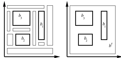
[image:25.612.156.404.73.192.2]b
Figure 1: Basic functional partitioning vs. functional partitioning.
much information is to “pave”C using strongly non-redundant subsets ofA, because every extra elementha
0 ;b
0
iadded toP leads to a loss of information for every token “covered” by a
0
. This is illustrated by the left part of figure 1 in the case of the interval lattice I(Z2
). But this pavement can turn out to be much too complicated when working with sophisticated lattices such as the linear inequalities lattice for instance. Worse, it can even be impossible to define such a pavement for atomic lattices that do not have a strongly non-redundant basis. What we would like to do is therefore to map small regionsfa
i g
i2I of
Cto a given set of valuesfb i
g i2I, while defining some kind of default valueb
0
for a larger and possibly overlapping areaa 0
, as illustrated by the right part of figure 1. This can be achieved by generalizing the definition of the meaning functionΓto every elementP of P(A;B) by:
Γ(P)(c) = M P[
c]
whereM P :
A!Bis defined by:
M P(
x) = F
a2A(P) a^x6=?
D P(
a^x;a)
and D
P(
u;v) = uP \
(u;v)
Given two abstract control pointsu andv,D P(
u;v) is equal to the greatest lower bound of the abstract valuesbassociated with the abstract control pointsathat belong to the (possibly empty) convex subset fx : u x vg. It is easy to see that this function is increasing in its first argument and decreasing in its second argument. The functionM
P is therefore monotonic and maps every abstract control pointx 2 A to the union of the abstract values
b associated with the minimum elementsa 2 A(P) such that x^a 6= ?. The meaning of a representation in Pnr(A;B) is thus identical to the meaning defined in the previous section, since every element of a non-redundant domain A(P) is minimum. The meaning of M
P for the representationP = fha;bi;ha
0 ;b
0 i;ha
00 ;b
00
igand three particular valuesa =[2;13], a
0
=[10;18] anda 00
=[6;21], is illustrated in figure 2 in the case of the interval lattice I(Z). The functionM
P maps an abstract control point, represented by a point on the plane using the usual encoding of intervals:
b
b
0 2 5 6 9 10 13 14 18 19 21 22
a,b
[image:26.612.94.506.67.256.2], a b ,b a b b b b b b b b b b
Figure 2: Meaning ofM P for
P =fha;bi;ha 0 ;b 0 i;ha 00 ;b 00 ig.
to an abstract value inB. The functionΓ(P) : Z ! B maps every integer kto M P[
k], where the token [k] = [k ;k] is the one-point interval. Note how the intervals belowa
0 are “protected” from the valueb
00
associated with the abstract control pointa 00
.
The problem however with this new meaning function Γ is that it is not monotonic over P(A;B). Intuitively, non-monotonicity arises when an element ha
0 ;b
0
i is added to a representationP anda
0
“masks” a region previously mapped to a value greater thanb 0
. This would be the case for instance in figure 2 ifha
0 ;b
0
iwas added tofha;bi;ha 00
;b 00
igandb 0
<b 00
. In order to avoid this situation, one can require that b
0
be greater than S P(
a 0
), where the
smallest safe valueS P(
x) is defined by:
S P(
x) =
G
a2A(P) ?<xa
D P(
x;a)
Intuitively, this condition ensures that the new valueb 0
is at least the union of every value that
a 0
could mask, i.e., the values associated with the minimum elements inA(P) that are above
a 0
. This intuition can be formalized by defining the relationover P(A;B) as follows:
P P 0
() (
8ha;bi2P ; 9ha 0
;b 0
i2P 0
: a=a 0
^ bvb 0
8ha 0
;b 0
i2P 0
: a 0
62A(P) =) b 0 wS P( a 0 )
Note that sinceS P(
a) =P(a) for every ain the domain of P, this condition could also be written as follows:
P P 0
() (
A(P)A(P 0 ) 8ha 0 ;b 0
i2P 0 : b 0 wS P( a 0 )
Proof. Let us first show thatΓis monotonic over P(A;B). So let us suppose thatP P 0
. ThenA(P) A(P
0
), and for everyx2Asuch thatx6=?:
8 < : S P 0(
x) w F
a2A(P) ?<xa
D P
0(
a^x;a)
M P
0( x) w
F a2A(P) a^x6=?
D P
0(
a^x;a)
But for everya2A(P) such that eitherx^a6=?or?<xa:
D P
0(
a^x;a) = u ha 0 ;b 0 i2P 0 a^xa 0 a (b 0 )
Let us now suppose that there exists ha 0
;b 0
i 2 P 0
such that a^x a 0
a. Then by hypothesis: b 0 w S P( a 0 ) = G a 00
2A(P) a 0 a 00 D P( a 0 ;a 00 ) w G a 00
2A(P) a 0 a 00 a D P( a 0 ;a 00 )
Buta^xa 0
a 00
aimplies thatD P(
a^x;a)vD P(
a 0
;a 00
), and sincea2A(P), the setfa
00
2A(P) :a 0
a 00
agis non-empty and thus:
b 0
w D P(
a^x;a)
which implies that:
D P
0(a^x;a) w D P(
a^x;a)
and therefore: (
S P
0(
x) w S P(
x) M
P 0(
x) w M P(
x) Consequently, sinceS
Q(
?) =M Q(
?)=?for every representationQ, thenM P vM P 0, S P v S P
0, and Γ is monotonic over P(
A;B). Finally, being trivially reflexive and antisymmetric, let us prove that it is also transitive. So letP P
0 P
00
. Then for every
ha 00
;b 00
i2P 00
such thata 00
62A(P), eithera 00
2A(P 0
), and thusb 00 wb 0 wS P( a 00
), or else:
b 00 w S P 0( a 00
) w S P(
a 00
)
which proves thatP P 00
.
We have proven that (P(A;B);) is a partial order, but we must note that the meaning function is not strictly monotonic, i.e., one can find two distinct representations such thatP
1 P
2 and
Γ(P 1)
=Γ(P
2). This holds for instance whenever b 1 <b 2 for: P i
= fh[1;1];bi;h[2;3];b 0
i;h[1;3];b i
ig (i2f1;2g)
since:
Γ(P 1)
= Γ(P 2)
= f17!b;27!b 0
;37!b 0
g
b b b b b1 b2 b3 b1 b2 b3 b3 b1 b2 b3 b1 b2 b3 a
a) = a3
b b b b b a >
a < < a and
c) 2 3 a a d) a <2 a < a3
a 3
2
[image:28.612.112.480.78.285.2]b) a < < a and a =a
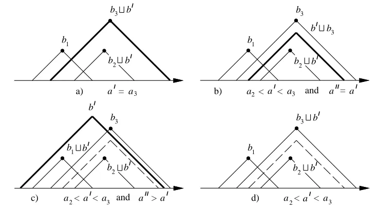
Figure 3: Widening in a functional partitioning framework.
control points are added and never removed during a given computation. Moreover, the information associated with each control point is only allowed to increase. Finally, we have a very easy criterion to check whether or not a pairha;bi2AB can be safely added to a representation, which is very important if one wishes to be able to generalize at some point of the computation. What we need now is to define elementary widening operators, i.e., operators such that: P P rP
0
andΓ(P 0
)vΓ(P rP 0
).
In the rest of this section, we shall only consider finite representations, for they have the greatest practical interest, and for the sake of simplicity, we start by definingP
00
=PrP 0
for a singletonP
0 =fha
0 ;b
0
ig. There are basically three cases in the definition ofP 00
. Each one is illustrated in figure 3, where we have takenA=I(Z), andP =fha
1 ;b
1 i,ha
2 ;b
2 i,ha
3 ;b 3 ig. Ifa 0
2A(P), then for everyha;bi2P such thataa 0
, the replacement ofbby any element greater thanb
0
tbensures that the meaning ofP 00
is greater than the meaning offha
0 ;b
0
ig, and at the same time thatP P 00
(fig. 3a).
Ifa 0
62A(P). Suppose one wishes to add this new abstract control point to the domain of the current representationP. Obviouslyha
0 ;b
0
icannot simply be added to P. But adding any pairha
00 ;b
00
isuch thata 00 a 0 andb 00 wb 0 tS P( a 00
) will ensure thatP P 00
. However, as in the previous case, everyha;bi2P such that aa
00
may “mask” the valueb
0
to several elements of the basis. Hence, each valuebmust be replaced by an element greater thanb
0
tbto ensure that the meaning ofP 00
is greater than the meaning offha
0 ;b
0
ig(fig. 3b and 3c).
There are cases however where a 0
62 A(P) but one does not want to add a 0
representations. There are then two subcases to consider. If (a 0
) C(P), every control pointcrepresented bya
0
is already represented by at least one elementasuch thatha;bi2P and [c]a, and replacingbbybtb
0
will ensure that the meaning ofP 00 is greater than the meaning offha
0 ;b
0
ig— provided of course that, as in the previous cases, everyb
00
such that ha 00
;b 00
i 2P anda 00
abe replaced by an element greater thanb
0 tb
00
(fig. 3d). But if(a 0
)6C(P), then the region defined bya 0
contains “new” control points, and there is no way to avoid the addition ofa
0
toA(P). The previous case must thus be applied, choosing for instancea
00 =>. Note that, in practice, the test(a
0
) C(P) will always be approximated, and a given abstract control point a
0
will not be added to the domain of P only if there exists
ha;bi 2 P such that a 0
a. Such an approximation will thus generally imply the non-stability of the widening operator (cf. section 3).
This definition shows that functional partitioning is well suited to generalization processes, for it enables one to easily generalize without losing too much information. In order to complete our framework, we now defineP rQfor any finite representationQ2P(A;B) by arbitrarily numbering the elementsha
i ;b
i
i,i2[1;k] ofQ, and adding them one at a time toP, i.e.:
PrQ = ((PrQ 1)
)rQ k whereQ i =fha i ;b i
ig. This definition trivially implies that:
PrQ ((PrQ 1)
)rQ k 1
P
and thanks to the next theorem:
Γ(P rQ) = Γ(((P rQ 1)
)rQ k) w Γ(Q
1)
ttΓ(Q k) w Γ(Q
1
[[Q k) = Γ(Q)
which shows that condition iv) of definition 1 is satisfied.
Theorem 11 For everyQ 1
;Q 2
2P(A;B) such thatQ 1
[Q 2
2P(A;B):
Γ(Q 1
[Q 2)
v Γ(Q 1)
tΓ(Q 2)
Proof. We first remark that for everyu;v2A:
(Q 1
[Q 2)
\
(u;v) = Q 1
\
(u;v)[Q 2
\ (u;v)
thus: D Q 1 [Q 2
(u;v) = D Q
1
(u;v)uD Q
2
(u;v) v D Q
1
(u;v); D Q
2 (u;v)
and therefore: M Q 1 [Q 2( x) =
F a2A(Q
1 [Q 2 ) a^x6=? D Q 1 [Q 2(
a^x;a)
= F
a2A(Q 1) a^x6=?
D Q1[Q2(
a^x;a)t F
a2A(Q 2) a^x6=?
D Q1[Q2(
a^x;a)
v M
Q1(
x)tM Q2(
x) which proves thatΓ(Q
1 [Q
2) vΓ(Q
1) tΓ(Q
a) b)
c) d)
a a
1 2
3
[image:30.612.189.411.74.261.2]a a
Figure 4: Widenings over Pnr(I(Z
2 )).
5 Applications
We are now going to present two possible applications of dynamic partitioning. The first one is simply the application of basic partitioning to the bi-dimensional interval lattice I(Z2
). Its interest is rather academic, but we shall use this example to illustrate how widening operators can be effectively built. In the second example, we will show how a precise description of the input/output behavior of a program function can be computed using functional partitioning. This example will exemplify the case where the shape of a program invariant cannot be predicted and has to be considered as an output of the fixed point computation itself.
5.1 Multi-intervals
The aim of this section is to show how sets of bi-dimensional intervals can be used to represent sets of integer pairs. Following the method developed in section 4.1, we can either use non-redundant subsets or strongly non-redundant subsets of I(Z2
). Note that strongly non-redundant subsets of I(Z2
) are always larger than non-redundant subsets. We are going to illustrate the ideas that can be used to build elementary widening operators over such subsets. Figure 4a shows an elementP =fa
1 ;a
2 ;a
3
gof Psnr(I(Z 2
)) plus an extra elementa 0
2I(Z 2
). We wish to calculateP
0
= P rfa 0
g. Figure 4b illustrates how P 0
can be defined using a join-like operator. Note that such an operator might be very difficult to implement. So let us focus on Pnr(I(Z
2
)). We shall define two elementary operators. The first oner
j (fig. 4c) behaves like a join operator and shall be used in the first steps of a computation. The second oner
g (fig. 4d) computes a generalization as follows. Using the widening operator
rIover
I(Z2
) defined in section 2, one first computesa 00
=( W
P) rIa 0
. Intuitively, W
P is used as a reference to determine in “which direction”a
0
is “moving”. Of course, different references can be used, such as the most recently added elements ofP for instance. Finally,P
0
Figure 5: Safe representation of lfp(Φ).
by removing the redundant elements ofP[fa 00
g. We shall use these two elementary widening operators to compute a non-trivial, safe and finitely represented approximation of the least fixed point ofΦ: P(N2
)!P(N 2
) defined by:
Φ(M) = fh2;1i;h2;2ig[fhbxy=2c;x+yig hx;y i2M
This least fixed point cannot be finitely represented in any usual lattice used for modeling sets of integer pairs, such as the linear inequalities lattice of Cousot and Halbwachs [3] for instance. But one can very easily define a safe approximationΦ#ofΦby:
Φ#(
P) = fh[2;2];[1;2]ig[fΦ
#
1( X ;Y)g
hX ;Yi2P
where:
Φ#
1([ i;s];[i
0 ;s
0
]) = h[bii 0
=2c;bss 0
=2c];[i+i 0
;s+s 0
]i
Then, using the framework of section 3 with the widening operator:
r = (r j 3
r g !
) = (r j
;r j
;r j
;r g
)
one can finitely compute the following non-trivial approximation displayed in figure 5:
n
h[2;2];[1;2]i; h[1;2];[3;4]i; h[1;4];[4;6]i;h[2;12];[5;10]i; h[5;!
+]
;[7;!
+]
i o
5.2 Minimal function graphs
We are now going to present an application of functional partitioning to interprocedural abstract interpretation, which in fact originally motivated this work. Let us suppose that one has a program functionΦ : Z ! Z
? such as the
fun Mc n = if (n > 100) then n-10
else
Mc(Mc(n + 11))
We wish to determine a safe approximation of the minimal function graph ofΦfor a given set of input data specifications. We are not going to formally describe a minimal function graph semantics but rather give an intuition about the way finite representations of minimal function graphs can be computed using functional partitioning. As hinted at the end of section 2, we shall abstract minimal function graphs using representations in P(I(Z);I(Z)), and input data specifications using representations in Pnr(I(Z)). So let us suppose that we have an initial
representationI
0 of the set of input data specifications. We can define the first representation of the minimal function graph ofΦwith respect to the input data specificationI
0by:
P 0
= fhi 0
;?ig i
0 2I
0
The meaning of a representationP is the one introduced in section 4.3, that is:
Γ(P)(n) = M P[
n;n]
where:
M P(
x) =
_^
hi;v i2P x^i6=?
fv 0
: (x^i)i 0
ig hi
0 ;v
0 i2P
Note that, contrary to what is proposed in Jones and Mycroft [10], we have not introduced a special value “!” to denote non-termination. Therefore, at the end of the computation, Γ(P)(n) =?either means thatΦhas never been called withnas argument or that it has been called and looped. Note that this is not too important since these two interpretations can be easily distinguished by looking at the domain of the representation. The approximate minimal function graph is therefore the limit of the increasing chain defined by:
P k+1
= Φ
#(
P k) whereΦ#(P) is defined as follows:
1) For everyhi;viinP, an updated valuev 0
wvofvis computed by applying the definition ofΦ to the set of values denoted byi and replacing the values of the recursive calls
Φ(i 0
) byM P(
i 0
). The latter is the best approximation ofΦ(i 0
) that can be given using the current approximation ofΦ.
2) ThenΦ#(P) =fhi;vrIv 0
ig hi;v i2P
r k
fhi 0
;?ig i
0 2I
0, where I
0
is the set of new abstract control points over whichΦhas been called in step 1.
In other words, we compute an updated approximation v 0
that recursive calls have generated new abstract control pointsi 0
by inserting these intervals into the representation.
The insertion of the updated value v 0
can be done for instance in a fairly simple way by using the usual widening operatorrIover I(Z) defined in section 2, and replacinghi;viin the initial representation byhi;vrIv
0
i, in order to make sure that the increasing chain of abstract values (v;v rI v
0
;. . .) will be eventually stable. Of course, at the beginning of the iteration sequence, it is also safe to replacehi;vibyhi;v_v
0 i. The insertion of the new abstract control pointsi
0
into the representation is more subtle, and uses the elementary widening operatorrdefined in section 4.3. Obviously, it is generally unsafe to add directly hi
0
;?i into the representation since, as discussed in section 4.3, i 0 might “mask” one of the intervalsiin the domain of the representation and thus invalidate its meaning. The smallest pair that can be safely inserted is thereforehi
0 ;S
P( i
0
)i. But abstract control points themselves need to be generalized in order to enforce a finite computation, and at some point of the iteration sequence, we will have to replace the intervali
0
by a greater one
i 00
, e.g., the maximum element >. This can be formalized by introducing three elementary widening operators defined as follows.
(r
a) Add the pair hi 0 ;S P( i 0
)i. This is the most precise, join-like, widening operator.
(r
b) When it is safe not to add i
0
, i.e., when the region covered byi 0
is already covered by the domain ofP, then do nothing, otherwise generalize by addinghi
00 ;S
P( i
00
)i, where
i 00
i 0
. A good choice can be for instancei 00
=( W
A(P))_i 0
, i.e., the smallest interval representing all the values over which Φ has been computed so far, in which case
S P( i 00 )=?. (r
c) Finally, to avoid adding an infinite number of abstract control points, one can use the widening operator over the intervals and addh(
W
A(P))rI i 0
;?i.
Of course, the choice of the sequence of elementary widening operators is essential. The first elementary widening operatorr
awill generally be used at the beginning of the computation, and r
c will systematically be used at the end. Moreover, it is often useful, after having generalized usingr
c, to make a few more precise steps using r
aor r
b. The motivation behind this choice is that once the domain of the minimal function graph has been delimited, a few more precise steps are generally needed to determine the abstract control points that are useful to precisely describe this graph and allow these intervals to “propagate” along recursive calls.
Finally, note that the insertion of the updated abstract valuesv 0
and the insertion of the new abstract control pointsi
0
can be freely mixed in pratice, and newly generated control points can be added on the fly to the representation without problem.
The widening operator that we have described turns the functional partitioning framework into a tractable framework. So for instance, using the widening operator (r
c r a r c !
), one can
graph ofLoopfor the input data specificationf[0;0]g:
n
h[0;0];[100;100]i;h[0;!
+]
;[100;!
+]
i;h[1;1];[100;100]i;h[1;100];[100;100]i o
which has the following meaning:
i Loop(i) 0n100 [100;100]
100<n [100;!
+]
This result is interesting in that it shows that the exact information:Loop[0;100]=[100;100] has been obtained, as opposed to section 2, and this has been achieved without the help of a narrowing operator. However, contrary to the result of section 2, the approximate minimal function graph seems to indicate that the computation ofLoop(0) might require computing
Loop for values greater than 100, but starting this time from the input data specification f[0;100]g, and using the “brute force” widening operator (r
c !
) we can compute the following representation:
n
h[0;100];[100;100]i o
which invalidates this interpretation. Similarly, using the widening operator (r c
r a
2 r
c !
) one can compute, after 4 iterations, the following representation of the minimal function graph of
Mcfor the input specificationf[0;50]g:
n
h[0;50];[91;91]i;h[0;!
+
10];[91;!
+]
i;h[11;111];[91;101]i;h[11;61];[91;91]i;
h[22;72];[91;91]i;h[22;111];[91;101]i;h[91;101];[91;91]i o
This representation has the following meaning:
n Mc(n) n<0 ? 0n72 [91;91] 73n90 [91;101] 91n101 [91;91] 102n111 [91;101]
112n [91;!
+
10]
which is a good and safe approximation of the exact meaning ofMc, i.e.:
Mc(n) = (
n 10 if n>101 91 otherwise
call toMc, that is, the main call toMcand the two recursive calls. This formally corresponds to having three mutually recursive functionsMc1,Mc2andMc3with the following definition:
if (n > 100) then n-10
else
Mc3(Mc2(n + 11))
and describing each of these functions by a pair of intervals representing all of the function’s inputs and all of the function’s outputs. The result obtained is the following:
Mc1 : h[0;50];[91;!
+
20]i Mc2 : h[11;!
+]
;[91;!
+
10]i Mc3 : h[91;!
+
10];[91;!
+
20]i
This quite mediocre result can be explained by noting that the induction property:
8n2[91;101] : Mc(n)=91
has not been inferred by the framework because the number of interval pairs was fixed in
advance. This phenomenon can be worked around by using an ad-hoc input data specification,
namelyf[0;100]g, which gives the following, optimum, result:
Mc1 : h[0;100];[91;91]i Mc2 : h[11;111];[91;101]i Mc3 : h[91;101];[91;91]i
However, this “trick” is not necessary when using the functional partioning framework, since this framework infers the interesting program properties by itself, and automatically determines the number of interval pairs needed to describe the program invariant. Howevever, it is worth mentioning that the widening operator has a major impact on the result’s quality, and for instance, the “brute force” widening operator would only compute, after 2 iterations, the following, mediocre but concise, representation:
n
h[0;50];[91;!
+
10]i;h[0;!
+]
;[91;!
+
10]i o
with the obvious meaning:
8n2[0;!
+] :
Mc(n) 2[91;!
+
10]
This example shows that the data-oriented approach of dynamic partitioning is much more versatile than the syntax-oriented approach of static partitioning, and generally gives better results. But on the other hand, static partitioning guarantees the size of the least fixed point’s representation, and can lead to faster analyses. Finally, note that the two approaches can be easily mixed. For example, using the widening operator (r
c r
a r
c !
Mc1 : fh[0;50];[91;91]ig
Mc2 : fh[11;61];[91;91]i;h[11;!
+]
;[91;!
+
10]i; h[22;72];[91;91]i;h[22;111];[91;101]ig Mc3 : fh[91;101];[91;91]ig
which have the following, coalesced meaning, obtained by intersecting their individual meanings:
n Mc(n) n<0 ? 0n72 [91;91] 73n90 [91;101] 91n101 [91;91] 102n111 [91;101]
112n [91;!
+
10]
6 Conclusion
We have presented a technique that enables rich abstract interpretation frameworks to be built from simpler ones even in cases when one has no indication about what such frameworks should look like. We believe in particular that functional partitioning is of great interest to interprocedural abstract interpretation for it incrementally builds finite, non-trivial representations of minimal function graphs and monotonic functions. More generally, the representation framework can be used every time there is no canonical representation of abstract program properties and the equivalence test over these properties is intractable or very costly.
References
1. Fran¸ccois Bourdoncle: “Interprocedural Abstract Interpretation of Block Structured Lan-guages with Nested Procedures, Aliasing and Recursivity”, Proc. of the International
Workshop PLILP’90, Lectures Notes in Computer Science 456, Springer-Verlag (1990)
2. Patrick and Radhia Cousot: “Abstract Interpretation: a unified lattice model for static analysis of programs by construction of approximative fixpoints” in Proc. of the 4th ACM
Symp. on POPL (1977) 238–252
3. Patrick Cousot and Nicolas Halbwachs: “Automatic discovery of linear constraints among variables of a program”, in Proc. of the 5th ACM Symp. on POPL (1978) 84–97
4. Patrick Cousot: “M´ethodes it´eratives de construction et d’approximation de points fixes d’op´erateurs monotones sur un treillis. Analyse s´emantique de programmes”, Ph.D. Thesis, Universit´e Scientifique et M´edicale de Grenoble (1978)
5. Patrick and Radhia Cousot: “Static determination of dynamic properties of recursive procedures”, Formal Description of Programming Concepts, North Holland Publishing Company (1978) 237–277
6. Patrick Cousot: “Semantic foundations of program analysis” in Muchnick and Jones Eds.,
Program Flow Analysis, Theory and Applications, Prentice-Hall (1981) 303–343
7. G. Gierz, K.H. Hofmann, K. Keimel, J.D. Lawson, M. Mislove, D.S. Scott: “A Com-pendium of Continuous Lattices”, Springer-Verlag (1980)
8. C.A. Gunter, D.S. Scott, “Semantic Domains”, in Handbook of Theoretical Computer
Science, Chapter 12, Elsevier Science Publishers B.V. (1990) 635–673
9. Neil D. Jones and Steven Muchnick: “A Flexible Approach to Interprocedural Data Flow Analysis and Programs with Recursive Data Structures”, in Proc. of the 9th ACM Symp.
on POPL (1982)
10. Neil D. Jones and Alan Mycroft: “Data flow analysis of applicative programs using minimal function graphs” in Proc. of the 13th ACM Symp. on POPL (1986) 296–306
11. Alan Mycroft and Flemming Nielson: “Strong Abstract Interpretation Using Power Domains (Extended Abstract)”, Proc. 10th ICALP, Lectures Notes in Computer Science 154, Springer-Verlag (1983) 536–547