WRL 89 13 pdf

WRL

Research Report 89/13

The Distribution of

Instruction-Level and

Machine Parallelism

and Its Effect on

Performance

research relevant to the design and application of high performance scientific computers. We test our ideas by designing, building, and using real systems. The systems we build are research prototypes; they are not intended to become products.

There is a second research laboratory located in Palo Alto, the Systems Research Cen-ter (SRC). Other Digital research groups are located in Paris (PRL) and in Cambridge, Massachusetts (CRL).

Our research is directed towards mainstream high-performance computer systems. Our prototypes are intended to foreshadow the future computing environments used by many Digital customers. The long-term goal of WRL is to aid and accelerate the development of high-performance uni- and multi-processors. The research projects within WRL will address various aspects of high-performance computing.

We believe that significant advances in computer systems do not come from any single technological advance. Technologies, both hardware and software, do not all advance at the same pace. System design is the art of composing systems which use each level of technology in an appropriate balance. A major advance in overall system performance will require reexamination of all aspects of the system.

We do work in the design, fabrication and packaging of hardware; language processing and scaling issues in system software design; and the exploration of new applications areas that are opening up with the advent of higher performance systems. Researchers at WRL cooperate closely and move freely among the various levels of system design. This allows us to explore a wide range of tradeoffs to meet system goals.

We publish the results of our work in a variety of journals, conferences, research reports, and technical notes. This document is a research report. Research reports are normally accounts of completed research and may include material from earlier technical notes. We use technical notes for rapid distribution of technical material; usually this represents research in progress.

Research reports and technical notes may be ordered from us. You may mail your order to:

Technical Report Distribution

DEC Western Research Laboratory, UCO-4 100 Hamilton Avenue

Palo Alto, California 94301 USA

Reports and notes may also be ordered by electronic mail. Use one of the following addresses:

Digital E-net: DECWRL::WRL-TECHREPORTS

DARPA Internet: [email protected]

CSnet: [email protected]

UUCP: decwrl!wrl-techreports

Machine Parallelism and Its Effect on Performance

Norman P. Jouppi

July, 1989

This paper examines non-uniformities in the distribution of instruction-level and machine parallelism. Non-uniformities in instruction-instruction-level paral-lelism include variations between benchmarks, variations within benchmarks, and variations by instruction class. Non-uniformities in machine-level parallelism include variations in latency between different operations, and variations in parallel execution capability depending on the instruction opcode. The results presented in this paper were obtained with a parameterizable code reorganization and simulation system.

The discussion of machine parallelism is based on the concepts of super-scalar and superpipelined machines. Supersuper-scalar machines can issue several instructions per cycle. Superpipelined machines can issue only one instruc-tion per cycle, but they have cycle times shorter than the latencies of their functional units. These two techniques are shown to be roughly equivalent ways of exploiting instruction-level parallelism. The average degree of

superpipelining metric is introduced to account for the non-unit operation

latencies present in most machines.

In this paper a methodology for quickly estimating machine performance is developed. A first order estimate is based on the average degree of super-pipelining. A second order model corrects for the effects of non-uniformities in instruction-level and machine parallelism and is shown to be accurate within 25% for three widely different machine pipelines: the CRAY-1, the MultiTitan, and a dual-issue superscalar machine.

This is a preprint of a paper that will appear in the

IEEE Transactions on Computers, Special

1960’s and early 1970’s [14, 12, 2]. Recently approaches to exploiting instruction-level paral-lelism have again become increasingly popular areas of research [9, 11, 13, 17, 1], as well as an emerging area of practice [8].

Much of this research has focused on the effects of adding parallel instruction issue capability to a specific pipeline. These results are not necessarily broadly applicable because of the specific machine-dependent timing assumptions made in the context of a specific machine pipeline. For example, in studies which start from a CRAY-1 baseline, the latency of scalar addition is three cycles and the load latency is eleven cycles. But what do parallel issue studies for these pipeline characteristics imply for a machine with a one-cycle add and a two-cycle load? By fixing the machine latencies and pipeline characteristics, these studies are restricted to a single line of increasing parallelism in what is actually a multidimensional space. In this work we attempt to present data which covers a large portion of the potential machine design space. Based on this data a methodology is developed that yields accurate performance estimates for a wide range of machine pipelines.

Another limitation of previous work is that many times the result data is presented in terms of averages. Average parallelism can provide a first approximation to machine performance, but non-uniformities in instruction and machine parallelism can also play a significant part in deter-mining machine performance. For example, consider a machine that requires an average of one addition per cycle for good performance on a benchmark. Is one adder enough for a machine to obtain good performance on this benchmark? If the additions are distributed such that in half the cycles there are no additions required, but in the other half there are two additions required, and such that in the non-addition cycles there are other instructions which use the results of the ad-ditions, then it makes sense to consider machines built with two adders. Thus the distribution of instruction-level parallelism is also an important area of work. In this paper we consider several non-uniformities in the distribution of instruction-level and machine parallelism and their effects on machine design and the estimation of a machine’s performance.

inter-block parallelism accessible, and these techniques are beyond the scope of this paper. However, once the inter-block instruction-level parallelism made available by these techniques is quan-tified, the performance estimation techniques developed in this paper are applicable based on the instruction-level parallelism present.

Section 2 describes the parameterizable compilation and simulation environment used to

*

measure the parallelism in benchmarks. In Section 3 we present a machine taxonomy helpful for understanding the duality of operation latency and parallel instruction issue. It also presents simulation data showing the duality of superscalar and superpipelined machines. Section 4 intro-duces important non-uniformities in instruction and machine parallelism. Typical distributions of these non-uniformities are presented from simulations using the parameterizable compilation and simulation system. In conjunction with the investigation of these non-uniformities a methodology for quickly estimating machine performance is developed. Resulting estimates are compared with simulated performance for several machines and differences are discussed. The importance of cache miss latencies and other memory system related effects are briefly con-sidered in Section 5. Section 6 summarizes the results of the paper.

2. Machine Evaluation Environment

The language system originally designed for the MultiTitan consists of an optimizing compiler (which includes the linker) and a fast instruction-level simulator. The compiler includes an inter-module register allocator and a pipeline instruction scheduler [15, 16]. For this study, we gave the system an interface that allowed us to alter the characteristics of the target machine. This interface allows us to specify details about the pipeline, functional units, cache, and register set. The language system then optimizes the code, allocates registers, and schedules the instructions for the pipeline, all according to this specification. The simulator executes the program accord-ing to the same specification.

To specify the pipeline structure and functional units, we need to be able to talk about specific instructions. We therefore group the MultiTitan operations into fourteen classes, selected so that operations in a given class are likely to have identical pipeline behavior in any machine. For example, integer add and subtract form one class, integer multiply forms another class, and single-word load forms a third class.

For each of these classes we can specify an operation latency. If an instruction requires the result of a previous instruction, the machine will stall unless the operation latency of the previous instruction has elapsed. The compile-time pipeline instruction scheduler knows this and schedules the instructions in a basic block so that the resulting stall time will be minimized.

Superscalar machines may have an upper limit on the number of instructions that may be issued in the same cycle, independent of the availability of functional units. We can specify this upper limit. If no upper limit is desired, we can set it to the total number of functional units.

We use our programmable reorganization and simulation system to investigate the perfor-mance of various machine organizations. We typically run eight different benchmarks on each different configuration. All of the benchmarks are written in Modula-2 except for yacc.

ccom Our own C compiler.

grr A printed-circuit board router.

linpack Linpack, double precision, unrolled 4x.

livermore The first 14 Livermore Loops, double precision, not unrolled. met Metronome, a board-level timing verifier.

stan The collection of Hennessy benchmarks from Stanford (including puzzle, tower, queens, etc.).

whet Whetsones.

yacc The Unix parser generator.

Unless noted otherwise, the effects of cache misses and systems effects such as interrupts and TLB misses are ignored in the simulations. For more information on the parameterizable com-pilation and simulation system see [6].

3. A Machine Taxonomy

There are several different ways to execute instructions in parallel. Before we examine these methods in detail, we need to start with some definitions:

operation latency The time (in cycles) until the result of an instruction is available for use as an operand in a subsequent instruction. For example, if the result of an Add instruction can be used as an operand of an instruction that is issued in the cycle after the Add is issued, we say that the Add has an operation latency of one.

simple operations The vast majority of operations executed by the machine. Operations such as integer add, logical ops, loads, stores, branches, and even floating-point addition and multiplication are simple operations. Not included as simple operations are instructions which take an order of magnitude more time and occur less frequently, such as divide and cache misses.

instruction class A group of instructions all issued to the same type of functional unit. issue latency The time (in cycles) required between issuing two instructions. This can

vary depending on the instruction classes of the two instructions.

3.1. The Base Machine

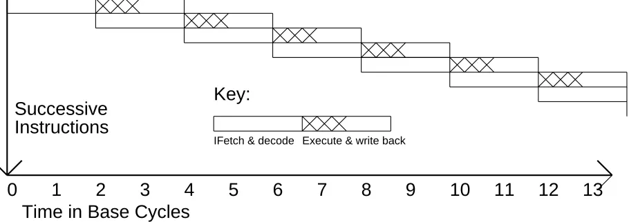
In order to properly compare increases in performance due to exploitation of instruction-level parallelism, we define a base machine that has an execution pipestage parallelism of exactly one. This base machine is defined as follows:

•Instructions issued per cycle = 1

•Simple operation latency measured in cycles = 1

•Instruction-level parallelism required to fully utilize = 1

satis-fying the requirements of a base machine is shown in Figure 1. The execution pipestage is cross-hatched while the others are unfilled. Note that although several instructions are executing con-currently, only one instruction is in its execution stage at any one time. Other pipestages, such as instruction fetch, decode, or write back, do not contribute to operation latency if they are bypassed, and do not contribute to control latency assuming perfect branch slot filling and/or branch prediction.

Successive

Instructions

9

Key:

12

11

10

8

7

6

5

4

3

2

1

0

Time in Base Cycles

Execute WriteBack Decode

IFetch

13

Figure 1: Execution in a base machine

3.2. Underpipelined Machines

The single-cycle latency of simple operations also sets the base machine cycle time. Although one could build a base machine where the cycle time was much larger than the time required for each simple operation, it would be a waste of execution time and resources. This would be an

underpipelined machine. An underpipelined machine that executes an operation and writes back

the result in the same pipestage is shown in Figure 2.

IFetch & decode

Key:

Execute & write back

Successive

Instructions

Time in Base Cycles

0

1

2

3

4

5

6

7

8

9

10

11

12

13

The assumption made in many paper architecture proposals is that the cycle time of a machine is many times larger than the add or load latency, and hence several adders can be stacked in series without affecting the cycle time. If this were really the case, then something would be wrong with the machine cycle time. When the add latency is given as one, for example, we assume that the time to read the operands has been piped into an earlier pipestage, and the time to write back the result has been pipelined into the next pipestage. Then the base cycle time is simply the minimum time required to do a fixed-point add and bypass the result to the next instruction. In this sense machines like the Stanford MIPS chip [4] are underpipelined, because they read operands out of the register file, do an ALU operation, and write back the result all in one cycle.

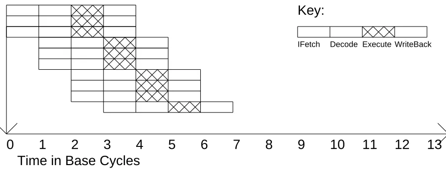
Another example of underpipelining would be a machine like the Berkeley RISC II chip [7], where loads can only be issued every other cycle. Obviously this reduces the instruction-level parallelism below one instruction per cycle. An underpipelined machine that can only issue an instruction every other cycle is illustrated in Figure 3. Note that this machine’s performance is the same as the machine in Figure 2, which is half of the performance attainable by the base machine.

IFetch Decode ExecuteWriteBack

Successive

Instructions

Time in Base Cycles

Key:

0

1

2

3

4

5

6

7

8

9

10

11

12

13

Figure 3: Underpipelined: issues < 1 instruction per cycle

In summary, an underpipelined machine has worse performance than the base machine be-cause it either has:

•a cycle time greater than the latency of a simple operation, or

•it issues less than one instruction per cycle.

For this reason underpipelined machines will not be considered in the rest of this paper.

3.3. Superscalar Machines

Time in Base Cycles

Key:

0

1

2

3

4

5

6

7

8

9

10

11

12

IFetch Decode ExecuteWriteBack

13

Figure 4: Execution in a superscalar machine (n=3)

In order to fully utilize a superscalar machine of degree n, there must be n instructions ex-ecutable in parallel at all times. If an instruction-level parallelism of n is not available, stalls and dead time will result where instructions are forced to wait for the results of prior instructions.

Formalizing a superscalar machine according to our definitions:

•Instructions issued per cycle = n

•Simple operation latency measured in cycles = 1

•Instruction-level parallelism required to fully utilize = n

A superscalar machine can attain the same performance as a machine with vector hardware. Consider the operations performed when a vector machine executes a vector load chained into a vector add, with one element loaded and added per cycle. The vector machine performs four operations: load, floating-point add, a fixed-point add to generate the next load address, and a compare and branch to see if we have loaded and added the last vector element. A superscalar machine that can issue a fixed-point, floating-point, load, and a branch all in one cycle achieves the same effective parallelism.

3.3.1. VLIW Machines

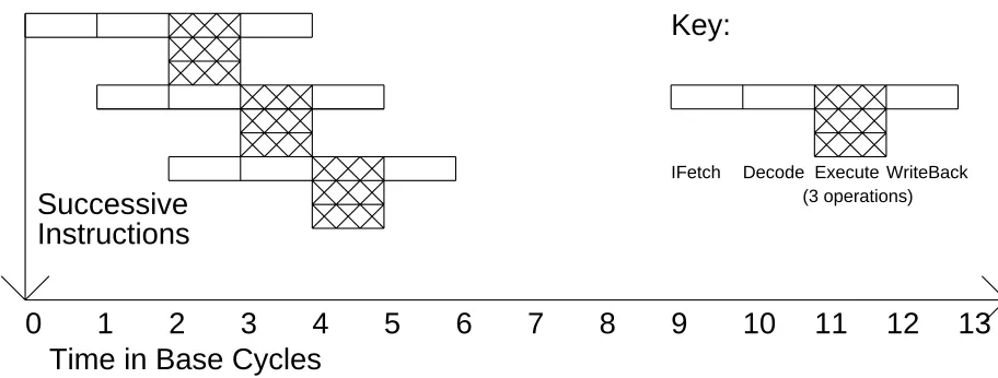
VLIW, or very long instruction word, machines typically have instructions hundreds of bits long. Each instruction can specify many operations, so each instruction exploits instruction-level parallelism. Many performance studies have been performed on VLIW machines [9]. The ex-ecution of instructions by an ideal VLIW machine is shown in Figure 5. Each instruction specifies multiple operations, and this is denoted in the Figure by having multiple crosshatched execution stages in parallel for each instruction.

VLIW machines are much like superscalar machines, with three differences.

(3 operations) IFetch Decode Execute WriteBack

Key:

Time in Base Cycles

13

12

11

10

9

8

7

6

5

4

3

2

1

0

Successive

Instructions

Figure 5: Execution in a VLIW machine

unit must look at a sequence of instructions and base the issue of each instruction on the number of instructions already issued of each instruction class, as well as checking for data dependencies between results and operands of instructions. In effect, the selection of which operations to issue in a given cycle is performed at compile time in a VLIW machine, and at run time in a super-scalar machine. Thus the instruction decode logic for the VLIW machine should be much simpler than the superscalar.

A second difference is that when the available instruction-level parallelism is less than that exploitable by the VLIW machine, the code density of the superscalar machine will be better. This is because the fixed VLIW format includes bits for unused operations while the superscalar machine only has instruction bits for useful operations.

A third difference is that a superscalar machine could be object-code compatible with a large family of non-parallel machines, but VLIW machines exploiting different amounts of parallelism would require different instruction sets. This is because the VLIW’s that are able to exploit more parallelism would require larger instructions.

In spite of these differences, in terms of run time exploitation of instruction-level parallelism, the superscalar and VLIW will have similar characteristics. Because of the close relationship between these two machines, we will only discuss superscalar machines in general and not dwell further on distinctions between VLIW and superscalar machines.

3.3.2. Class Conflicts

There are two ways to develop a superscalar machine of degree n from a base machine. 1. Duplicate all functional units n times, including register ports, bypasses, busses,

and instruction decode logic.

2. Duplicate only the register ports, bypasses, busses, and instruction decode logic.

same functional unit. If the busy functional unit has not been duplicated, the superscalar machine must stop issuing instructions and wait until the next cycle to issue the second instruc-tion. Thus class conflicts can substantially reduce the parallelism exploitable by a superscalar machine. (We will not consider superscalar machines or any other machines that issue instruc-tions out of order. Techniques to reorder instrucinstruc-tions at compile time instead of at run time are almost as good [2, 3, 16], and are substantially simpler than doing it in hardware.)

3.4. Superpipelined Machines

Superpipelined machines exploit instruction-level parallelism in another way. In a super-pipelined machine of degree m, the cycle time is 1/m the cycle time of the base machine. Since a fixed-point add took a whole cycle in the base machine, given the same implementation tech-nology it must take m cycles in the superpipelined machine. Figure 6 shows the execution of instructions by a superpipelined machine. Note that by the time the third instruction has been issued there are three operations in progress at the same time.

Formalizing a superpipelined machine according to our definitions:

•Instructions issued per cycle = 1, but the cycle time is 1/m of the base machine

•Simple operation latency measured in cycles = m

•Instruction-level parallelism required to fully utilize = m

IFetch Decode ExecuteWriteBack

Time in Base Cycles

Key:

Successive

Instructions

0

1

2

3

4

5

6

7

8

9

10

11

12

13

Figure 6: Superpipelined execution (m=3)

3.5. Superpipelined Superscalar Machines

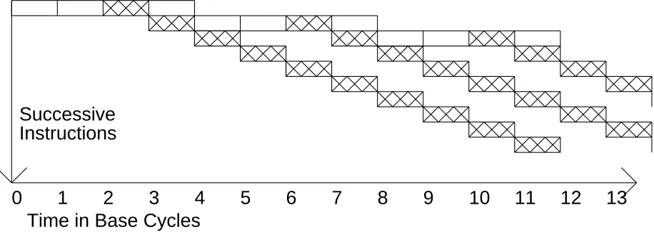
Since the number of instructions issued per cycle and the cycle time are theoretically or-thogonal, we could have a superpipelined superscalar machine. A superpipelined superscalar machine of degree (m,n) has a cycle time 1/m that of the base machine, and it can execute n instructions every cycle. This is illustrated in Figure 7.

Key:

Time in Base Cycles

13

12

11

10

9

8

7

6

5

4

3

2

1

0

Execute WriteBack Decode

IFetch

Figure 7: A superpipelined superscalar (n=3,m=3)

Formalizing a superpipelined superscalar machine according to our definitions:

•Instructions issued per cycle = n, and the cycle time is 1/m that of the base machine

•Simple operation latency measured in cycles = m

•Instruction-level parallelism required to fully utilize = n*m

3.6. Vector Machines

Although vector machines also take advantage of (unrolled-loop) instruction-level parallelism, whether a machine supports vectors is really independent of whether it is a superpipelined, su-perscalar, or base machine. Each of these machines could have an attached vector unit. However, to the extent that the highly parallel code was run in vector mode, it would reduce the use of superpipelined or superscalar aspects of the machine to the code that had only moderate instruction-level parallelism. Figure 8 shows serial issue (for diagram readability only) and parallel execution of vector instructions. Each vector instruction results in a string of operations, one for each element in the vector.

3.7. Supersymmetry

The most important thing to keep in mind when comparing superscalar and superpipelined machines of equal degree is that they have basically the same performance.

Successive

Instructions

Time in Base Cycles

0

1

2

3

4

5

6

7

8

9

10

11

12

13

Figure 8: Execution in a vector machine

three instructions in successive cycles. Each of these machines issues instructions at the same rate, so superscalar and superpipelined machines of equal degree have basically the same perfor-mance.

So far the assumption has been that the latency of all operations, or at least the simple opera-tions, is one base machine cycle. As we discussed previously, no known machines have this characteristic. For example, few machines have one cycle loads without a possible data interlock either before or after the load. Similarly, few machines can execute floating-point operations in one cycle. What are the effects of longer latencies? Consider the MultiTitan [5], where ALU operations are one cycle, but loads, stores, and branches are two cycles, and all floating-point operations are three cycles. The MultiTitan is therefore a slightly superpipelined machine. If we multiply the latency of each instruction class by the frequency we observe for that instruction class when we perform our benchmark set, we get the average degree of superpipelining. The average degree of superpipelining is computed in Table 1 for the MultiTitan and the CRAY-1. To the extent that some operation latencies are greater than one base machine cycle, the remain-ing amount of exploitable instruction-level parallelism will be reduced. In this example, if the average degree of instruction-level parallelism in slightly parallel code is around two, the Mul-tiTitan should not stall often because of data-dependency interlocks, but data-dependency inter-locks should occur frequently on the CRAY-1.

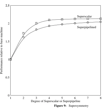
To confirm the duality of latency and parallel instruction issue we simulated the eight benchmarks on an ideal base machine, and on superpipelined and ideal superscalar machines of degrees 2 through 8. Figure 9 shows the results of this simulation. The superpipelined machine actually has less performance than the superscalar machine, but the performance difference decreases with increasing degree.

instruc-Instr. Fre- MultiTitan CRAY-1

class quency latency latency

logical 6% x 1 = 0.06 x 1 = 0.06 shift 9% x 1 = 0.09 x 2 = 0.18 add/sub 21% x 1 = 0.21 x 3 = 0.63 load 34% x 2 = 0.68 x11 = 3.74 store 15% x 2 = 0.30 x 1 = 0.15 branch 10% x 2 = 0.20 x 3 = 0.30

FP 5% x 3 = 0.15 x 7 = 0.35

Average Degree

of Superpipelining 1.7 5.4

Table 1: Average degree of superpipelining

1 2 3 4 5 6 7 8

Degree of Superscalar or Superpipeline 0

2.5

0.5 1 1.5 2 2.5

Performance relative to base machine

Superpipelined Superscalar

Figure 9: Supersymmetry

tions executing at the same time in the steady state, the superpipelined machine has a larger startup transient and it gets behind the superscalar machine at the start of the program and at each branch target. This effect diminishes as the degree of the superpipelined machine increases and all of the issuable instructions are issued closer and closer together. This effect is seen in Figure 9 as the superpipelined performance approaches that of the ideal superscalar machine with in-creasing degree.

IFetch Decode ExecuteWriteBack

Time in Base Cycles

Key:

Superpipelined

Superscalar

11

10

9

8

7

6

5

4

3

12

2

1

0

13

Figure 10: Start-up in superscalar vs. superpipelined

operations which can be performed in less time than a base machine cycle set by the integer add latency, such as logical operations or register-to-register moves. In a base or superscalar machine these operations would require an entire clock because that is by definition the smallest time unit. In a superpipelined machine these instructions might be executed in one super-pipelined cycle. Then in a superscalar machine of degree 3 the latency of a logical or move operation might be 3 times longer than in a superpipelined machine of degree 3. Since the latency is longer for the superscalar machine, the superpipelined machine will perform better than a superscalar machine of equal degree. In general, when the inherent operation latency is divided by the clock period, the remainder is less on average for machines with shorter clock periods.

overall preference to superpipelined machines for small degrees of machine parallelism, and a larger preference for increasing degrees of machine parallelism.

1 2 3 4 5 6 7 8

Multiple to which latencies are rounded 0

0.2 0.4 0.6 0.8 1

Relative performance

ideal superpipelined performance

ccom grr linpack livermore metronome stanford whetsones yacc

Figure 11: Loss in performance due to increased latency granularity

1 2 3 4 5 6 7 8 Instruction issue multiplicity

0 120

20 40 60 80 100

Performance (MIPS)

all latencies = 1

actual CRAY-1 latencies

Figure 12: Parallel issue with unit and real latencies

3.8. A First-Order Performance Approximation

An understanding of the average degree of superpipelining of a machine leads to a simple first-order method of estimating the performance of a machine. First, by multiplying the average degree of superpipelining (S ) by the degree of parallel issue (i.e., superscalar degree S ), we get_{P S} the average degree of machine parallelism (MP).

MP = S * S_{P S}

If the average parallelism in the benchmark (BP) exceeds the average parallelism of the machine, then usually most of the parallelism of the machine will be utilized and the perfor-mance will be limited by the parallelism of the machine. Similarly, if the average parallelism in the benchmark is less than the average parallelism of the machine, then the performance will be limited by the parallelism inherent in the benchmark. We can approximate the overall perfor-mance as two piecewise linear regions (see Figure 13). In the region on the left the perforperfor-mance is limited by the machine parallelism, and on the right the performance is limited by the benchmark parallelism. In other words, relative to a base machine with an equivalent cycle time,

if (BP >= MP) then performance = MP if (MP >= BP) then performance = BP

1 2 3 4 5 6 7 8 9 10 Average degree of machine parallelism

1 3

2

Performance relative to base machine performance limited by machine parallelism

performance limited by program parallelism

Figure 13: Piecewise linear approximation to performance vs. machine parallelism

a benchmark with BP equal to 2. From this information we can derive an estimate of the ab-solute performance of the processor (neglecting cache misses and other memory system or I/O factors). We can calculate the average CPI (cycles per instruction) of the machine by dividing its average degree of superpipelining by its performance relative to the base machine. For example, if a machine has an average degree of superpipelining of 4 and twice the performance of a base machine, then the machine will have an average CPI of 2. Similarly, if a superscalar machine has a average degree of superpipelining of 1 and outperforms a base machine by a factor of two, then it achieves 0.5 CPI on the average. Finally by dividing the number of cycles per second by the CPI we can get an absolute performance estimate in instructions per second. Since the ab-solute cycle time is a simple multiplicative factor in our performance comparisons, in the remainder of this paper we will discuss machine performance relative to a base machine with an equivalent cycle time.

As a second example, consider a dual-issue superscalar machine with the same pipeline latencies as the MultiTitan. Its average machine parallelism would then be twice that of the MultiTitan (assuming no class conflicts), giving MP = 3.4. This machine’s performance should be limited by the benchmark parallelism, since its average machine parallelism is larger than the average benchmark parallelism, 2.16. This would give an estimated speedup of 2.16 over a base machine with a cycle time 1.7 times larger. This would make its estimated CPI 0.79 (i.e., 1.7 / 2.16). The simulated performance was 0.91 CPI when ignoring cache misses. Thus the es-timated performance is about 15% less than the simulated performance.

As a third example consider the CRAY-1. It has an average degree of superpipelining of 5.4 on the eight benchmarks. This is greater than the average instruction-level parallelism present in the benchmarks. This means the performance will be limited by the benchmark parallelism, and a significant amount of the parallelism available in the machine will go unused. The CRAY-1 performance on the benchmarks should be 2.16 times that of a base machine with a cycle time 5.4 times that of the CRAY-1. This means that the average CPI of the CRAY-1 executing the benchmarks is estimated to be 2.50. Actual simulation of the benchmarks on the CRAY-1 yields a CPI of 3.75. This is 50% larger than the estimate.

What can cause this large error? Up to now the analysis has only considered averages. Unfor-tunately machine and instruction-level parallelism within benchmarks is not uniformly dis-tributed. For example, most of the latencies of the CRAY-1 are relatively short compared to the load latency of 11 cycles. Imagine three instructions that can be executed in parallel, and the instructions are a load, an add, and a logical operation. Although we could issue the load fol-lowed by the add and the logical operation in successive cycles, a wait for the result of the load would stall the issue of instructions for 8 more cycles. Thus the CPI for these three instructions is 11 (the delay of the load) divided by 3 (the number of instructions executed), or 3.67. This is much closer to the simulated performance.

1 2 3 4 5 6 7 8 9 10 Average degree of machine parallelism

1 3

2

Performance relative to base machine

Figure 14: Performance vs. machine parallelism with non-uniformities

4. Non-uniformities in Instruction-Level Parallelism

4.1. Variations in Parallelism by Benchmark

1 2 3 4 5 6 7 8 Benchmark

1 5

2 3 4

Average instruction-level parallelism

ccom grr

linpack

liver

met stan whet

yacc

Figure 15: Average instruction-level parallelism by benchmark

4.2. Variations in Machine Operation Latency

execution complete complete execution 7,8 execution complete 5,6 Parallel Non-uniform Serial Non-uniform Uniform 7,8 5,6 3,4 1,2

Operations <= 4 have latency = 3, operations > 4 have latency = 1 Odd operations have latency=3, even operations have latency=1 7 5 3,8 6 4 1,2 All operations have latency=2 13 12 11 10 3,4 1,2 8 7 6 5 4 3 2 1 9 8 7 6 5 4 Cycle 3 2 1

Figure 16: Variations in machine operation latency

To get a better understanding of the effects of non-uniform latencies, imagine a machine where the latency for one operation is much larger than the others. In the limit, the performance is not given by the long operation latency divided by the benchmark parallelism, but rather by the long latency divided by the parallelism between long latency operations (as was illustrated in Figure 16). For example, consider a machine where the latency of all operations is 1 except one operation has a latency of 1,000. Then the number of short latency instructions in parallel with a large latency instruction is basically insignificant for typical amounts of instruction-level paral-lelism (e.g., <4). The only important factor is the paralparal-lelism of these long latency operations between themselves. The first-order approximation which divides the latency of an operation by the benchmark parallelism (e.g., 2.16) will underestimate the time required for program execu-tion. In the limit, with no long latency operations in parallel with each other, the first-order approximation underestimates performance by a factor equal to the benchmark parallelism.

Figure 17 shows the average parallelism within typical instruction classes. This data was ob-tained by simulating an unlimited issue superscalar machine. For most benchmarks except the unrolled version of linpack, if an operation in a particular instruction class is executed, then the average number of instructions in the same class executable in parallel with the first operation is between 0.1 and 0.25. For example, the data for loads shows that on cycles in which there were a non-zero number of loads issued there were 1.25 loads issued on average. Note that this is not saying that on every cycle an average of 1.25 loads were issued, but only that whenever a load was issued there were 0.25 other loads in parallel with the load. The standard version of Linpack used has its inner loop unrolled four times, and so there are many operations of the same class executable at the same time in the inner loop. Similar behavior is expected in other unrolled benchmarks, but has not yet been verified.

1 2 3 4 5 6 7 8

Benchmark 1

4

1.5 2 2.5 3 3.5

Average parallelism by class

ccom grr linpack liver met stan whet yacc iadd/sub logic iload istore ext fload fstore fmul

Figure 17: Average parallelism within instruction classes by benchmark

Given the data in Figure 17 we can correct our performance estimate for time that the machine is stalled waiting for the completion of an operation with significantly larger than average latency. For example, consider the performance estimate of the CRAY-1 in section 3.8. The only operations with latency larger than the average degree of superpipelining in the CRAY-1 are load and FP operations. Table 2 shows the result of the correction calculation. (WCP is the within-class parallelism.)

be-Instr. Fre- x [ [CRAY-1 / avg.] - [Cray-1 / avg.]] = correction class quency [ [latency WCP ] [latency BP ]] to 1st order load 34% x ( ( 11 / 1.25 ) - ( 11 / 2.16) ) = 1.26 FP 5% x ( ( 7 / 1.25 ) - ( 7 / 2.16) ) = 0.12

Total common-class parallelism correction 1.38

Table 2: Calculation of non-uniform latency correction factor

tween different classes will increase the divider to a value larger than the common-class paral-lelism of 1.25 used in the calculation. This will reduce the magnitude of the overall CPI correc-tion. To the extent that the load latency is much larger than the other latencies, however, the importance of cross-class parallelism within long operations is reduced.

To summarize, when the performance is limited by the benchmark parallelism, non-uniformities in machine parallelism (e.g., latency) can cause errors in the estimated performance. By properly accounting for these non-uniformities in machine parallelism, we can lower the asymptote for this region and improve the accuracy of the performance estimate.

4.3. Variations in Aggregate Instruction Parallelism

The third non-uniformity we consider is non-uniformity in the cycle-by-cycle amount of in-struction parallelism. For example, consider the situation in Figure 18. Here the average num-ber of instructions executed in parallel is two. A machine with unlimited machine parallelism could execute this expression in three cycles. However, because this parallelism is not uniformly distributed with two instructions in parallel at each level in the expression graph, a machine that can only issue two instructions per cycle would take four cycles to execute the expression. Thus non-uniformities in instruction-level parallelism will decrease the performance achieved. This is especially true in the region where the machine parallelism is approximately equal to the average benchmark parallelism.

1 2 3

4 5

6

Instructions issued

Unlimited superscalar

1 2 3 4 Cycle

Degree 2 superscalar

1,2,3 4,5 6

1,2 3,4 5 6

Figure 18: Variations in the number of instructions executable in parallel

issue parallelism. We call this the single-issue bottleneck, and will discuss it further. The issue of more than three instructions per cycle is relatively rare. The notable exception to this is lin-pack which had a cycle with eight instructions issue in the inner loop. There were only a negli-gible number of cycles where more than ten instructions were issued in a cycle, so they are omitted from the graph.

Averaging the number of instructions executed in parallel for each benchmark from Figure 19 gives the average parallelism by benchmark shown in Figure 15. The spike at 2.16 is the hypothetical uniform distribution of parallelism at the average parallelism on the eight benchmarks. If a machine could issue exactly 2.16 instructions per cycle and the benchmark parallelism was a constant 2.16, then the performance would be 2.16 times that obtained by a base machine with the same cycle time. This performance point would be at the intersection of the two piecewise linear approximations.

1 2 3 4 5 6 7 8 9 10

Number of instructions issued 0

100

10 20 30 40 50 60 70 80 90

Instruction issue frequency percentage

hypothetical uniform distribution

ccom

PCBrouter

linpack

livermore

met

stanford

whetstones

yacc

Figure 19: Distribution of parallel instruction issue frequency

1 2 3 4 5 6 7 8 Instruction issue multiplicity

1 4

2 3

Superscalar performance realtive to base machine

ccom grr

linpack.unroll4x

livermore

metronome stanford

whetsones

yacc

Figure 20: Instruction-level parallelism by benchmark

One of the largest components of non-uniformity in instruction-level parallelism are single-issue bottleneck cycles where data dependencies neck down to a single instruction. Based on Figure 19, in a superscalar machine with unlimited parallel issue capability, single-issue bot-tlenecking occurs on about 40% of all cycles over a wide range of benchmarks. However if the degree of the superscalar machine is limited, code reorganization will migrate relatively uncon-strained instructions to be in parallel with bottlenecks instead of being executed in parallel with earlier instructions. Thus as the degree of the superscalar machine decreases from an unlimited number down to two, the number of single-issue cycles decreases. (Of course it becomes 100% for superscalar machines of degree 1.) This behavior was observed when superscalar machines of various degrees were simulated (see Figure 21).

1 5 10 15 20 25 30 32 Degree of superscalar machine

0 100

10 20 30 40 50 60 70 80 90

Percent of cycles with single issue

ccom

PCBrouter

linpack

livermore

met

stanford

whetstones

yacc

Figure 21: Frequency of single-issue cycles vs. machine parallelism

version of Figure 20 where the machine-limited performance asymptote has been adjusted for each benchmark based on the number of single-issue cycles in the benchmark at a machine paral-lelism of 2. These new asymptotes are much closer upper bounds to the the performance of the benchmarks than the old unit slope asymptote.

We can apply a correction for single-issue cycles to the earlier performance estimate for the MultiTitan CPU. In Section 3.8 its performance was estimated to be 1.00 CPI because its perfor-mance was limited by its own machine parallelism. Correcting just for single-issue cycles would decrease the performance improvement from 1.7 over a base machine to 1 plus 73% of the .7 extra machine parallelism, or 1.51 times a base machine with a 1.7 times larger cycle time. This is equivalent to a CPI of 1.13 (i.e., 1.7 / 1.51). Thus the correction for single-issue cycles reduces the difference between the estimated CPI (1.13) and the simulated CPI (1.22) to less than 10%.

1 2 3 4 5 6 7 8 Instruction issue multiplicity

1 4

2 3

Superscalar performance realtive to base machine

old asymptote average new asymptote

ccom grr

linpack.unroll4x

livermore

metronome stanford

whetsones

yacc

Figure 22: Single-issue correction for machine-parallelism limited asymptote

4.4. Variations in Parallelism by Instruction Class

A fourth important non-uniformity for machines with class conflicts is the distribution of in-structions by instruction class. In the example of Figure 23 the expression can be executed in three cycles by a superscalar machine of degree three with no class conflicts. Consider instead a superscalar machine with three instruction classes: load-store, arithmetic-logical-shift, and branches. If the superscalar machine can only execute at most one instruction of each class each cycle, it will take five cycles to execute the six instructions. This is a reduction of over 50% in the speedup obtained as compared to classless multiple issue capability.

6 4,5 1,2,3 Cycle 3 2 1 6 5 4 3 2

1 Load Load Load

Add Sub Store Classless superscalar 1 2,4 3 5 4 5 Instructions issued 6 Mem|ALU|branch class superscalar

Figure 23: Non-uniform distribution by instruction class

one data port to the memory system. Similarly, if the machine has separate floating-point and integer register files, this four-class structure may not require any additional ports to the register file over a non-superscalar machine (assuming each register file has 1 write and 2 read ports for ALU operations, 1 independent read/write port for loads and stores, and branches test condition codes). Machines with 16 classes have a class for each of the instruction types listed in Table 3. In the remainder of this section we refer to each machine by the 3-tuple of its superscalar degree, number of classes, and class multiplicity. For example, the leftmost machine structure is (1,X,1).

Machine structure 0 0.2 0.4 0.6 0.8 1 Relative performance

ideal superscalar performance

1 X 1 2 4 1 2 16 1 2 X 2 3 4 1 3 16 1 3 4 2 3 16 2 3 X 3 16 X 16 maximum issue number of classes class multiplicity ccom grr linpack livermore metronome stanford whetsones yacc

Machine Instructions

class in class

Load/Store CPU load, CPU store, transfer, FPU load, FPU store

CPU ALU CPU (integer) ops: add/sub, logical, shifts, multiply, divide

FPU ALU FPU (floating-point) ops: add/sub, multiply, divide, conversions

Branch branch/jump/JSR, trap

Table 3: The instruction classes of Figure 24

Figure 24 shows that class conflicts can have a very significant effect on machine perfor-mance. For example, machine (2,4,1) only exploits an average of 41% of the available instruction-level parallelism, and an average of 61% of the parallelism exploited by a machine of the same degree with no class conflicts (e.g., (2,X,2)). Similarly machine (3,4,1) only exploits 51% of the parallelism exploited by machine (3,X,3).

Simply increasing the degree of a superscalar machine has little effect on performance, unless the number of classes or their multiplicity are increased commensurably. For example, machine (3,4,1) has on average only 3% better performance than machine (2,4,1). This is not surprising, since the percentage of floating-point and branch instructions in most programs is lower than that of load/stores or CPU ALU operations to begin with, so even if all floating-point operations or branches could be executed in parallel with load/store and CPU operations, there would still be many cycles with only load/store and CPU operations issuing.

In general, increasing the multiplicity of the functional units is more important than increasing the number of instruction classes. For example, the increase in performance from increasing the multiplicity of functional units from 1 to 2 is greater than that from increasing the number of classes from 4 to 16. This is because when there are two copies of a functional unit, it can issue any two instructions of the class, whereas in a machine with many classes two instructions still may conflict. For example, machine (3,4,2) can issue any two load instructions in the same cycle, whereas machine (3,16,1) can only issue two load instructions if one is a CPU load and the other is an FPU load.

The impact of class conflicts has implications for the choice between superscalar and super-pipelined implementations. Since a supersuper-pipelined machine is less likely to have class conflicts than a superscalar machine (in general it is cheaper to pipeline a functional unit than to duplicate it), the effects of class conflicts can give a significant performance advantage to superpipelined machines over superscalar machines. For example, on average the machine (2,4,1) only attains 84% of the performance of a degree 2 superscalar machine without class conflicts, and machine (3,4,1) only attains 79% of the performance of a degree 3 superscalar without class conflicts.

5. Other Important Factors

Cache performance is becoming increasingly important, and it can have a dramatic effect on speedups obtained from parallel instruction execution. Figure 4 lists some cache miss times and the effect of a miss on machine performance. Over the last decade, cycle time has been decreas-ing much faster than main memory access time. The average number of machine cycles per instruction has also been decreasing dramatically, especially when the transition from CISC machines to RISC machines is included. These two effects are multiplicative and result in tremendous increases in miss cost. For example, a cache miss on a VAX 11/780 only costs 60% of the average instruction execution. Thus even if every instruction had a cache miss, the machine performance would only slow down by 60%! However, if a RISC machine like the WRL Titan [10] has a miss, the cost is almost ten instruction times. Moreover, these trends seem to be continuing, especially the increasing ratio of memory access time to machine cycle time. In the future a cache miss on a superscalar machine executing two instructions per cycle could cost well over 100 instruction times!

Machine cycles cycle mem miss miss per time time cost cost instr (ns) (ns) cycles instr

VAX11/780 10.0 200 1200 6 .6

WRL Titan 1.4 45 540 12 8.6

? 0.5 5 350 70 140.0

Table 4: The cost of cache misses

Cache miss effects decrease the benefit of parallel instruction issue. Consider a 2.0 CPI machine, where 1.0 CPI is from issuing one instruction per cycle, and 1.0 CPI is cache miss burden. Now assume the machine is given the capability to issue three instructions per cycle, to get a net decrease down to 0.5 CPI for issuing instructions when data dependencies are taken into account. Performance is proportional to the inverse of the CPI change. Thus the overall perfor-mance improvement will be from 1/2.0 CPI to 1/1.5 CPI, or 33%. This is much less than the improvement of 1/1.0 CPI to 1/0.5 CPI, or 100%, as when cache misses are ignored.

6. Concluding Comments

In this paper we have shown superscalar and superpipelined machines to be roughly equiv-alent ways to exploit instruction-level parallelism. The duality of latency and parallel instruction issue was documented by simulations. Ignoring class conflicts and implementation complexity, a superscalar machine will have slightly worse performance than a superpipelined machine of the same degree due to the larger cycle time granularity of the superscalar machine, although this is partially offset by the larger startup transient of the superpipelined machine. For example, reducing the granularity of the functional unit latencies in the CRAY-1 by factors of 2 to 4 results in a 10% to 15% performance loss, respectively. Moreover, if the superscalar machine has significant class conflicts these could further reduce the performance of a superscalar machine by 15% or 20% relative to a superpipelined machine of equal degree without conflicts.

Unit-parallelism bottlenecks in benchmarks can have a significant effect on machine perfor-mance. The effect of these constrictions in parallelism increases as the machine parallelism in-creases. For machines that can issue an unlimited number of instructions in parallel, single-instruction issue cycles typically accounted for 40% of all cycles.

Variations in machine parallelism (i.e., latency) were also investigated in conjunction with the development of a simple model of machine performance. The model estimates machine perfor-mance using a piecewise linear approximation.

In the first region, performance is limited by machine parallelism. The first-order perfor-mance estimate is simply the machine parallelism times that of the base machine perforperfor-mance at the equivalent cycle time. The accuracy of this estimate can be improved by considering the effect of non-uniformities in benchmark parallelism. The number of single-issue cycles is a use-ful correction factor.

In the second region, performance is limited by benchmark parallelism. The first-order perfor-mance is simply the benchmark parallelism times the perforperfor-mance of a base machine with the equivalent cycle time. The accuracy of this estimate can be improved by considering the effects of non-uniformities in machine parallelism. A correction factor can be computed using the latency of operations greater than the average degree of superpipelining, their frequency, and their frequency of occurrence in parallel with each other.

Cache misses and other memory system related effects are also very important contributors to machine performance. Much existing excellent work in this area can be used to augment the performance modeling of instruction-level and machine parallelism presented in this paper.

Overall, an understanding of non-uniformities in intra-basic-block instruction-level parallelism and machine parallelism allows the estimation of machine performance to within 15% of simu-lated performance for fully-pipelined machines without significant class or resource conflicts. Finally, a remaining area of research is the exploration of the non-uniformities in the distribution of inter-basic-block instruction-level parallelism obtained in code with large amounts data paral-lelism transformed into instruction-level paralparal-lelism through techniques such as aggressive loop unrolling, software pipelining, trace scheduling, or branch prediction.

7. Acknowledgements

David W. Wall provided the parameterizable compilation and simulation system used in this study, and largely contributed section 2. James E. Smith provided encouragement to examine the effects of increased cycle time granularity on supersymmetry. Richard Swan, David W. Wall, Jon Bertoni, and Mary Jo Doherty provided valuable comments on an early draft of this paper.

References

[1] Acosta, R. D., Kjelstrup, J., and Torng, H. C.

An Instruction Issuing Approach to Enhancing Performance in Multiple Functional Unit Processors.

[2] Foster, Caxton C., and Riseman, Edward M.

Percolation of Code to Enhance Parallel Dispatching and Execution.

IEEE Transactions on Computers C-21(12):1411-1415, December, 1972.

[3] Gross, Thomas.

Code Optimization of Pipeline Constraints.

Technical Report 83-255, Stanford University, Computer Systems Lab, December, 1983. [4] Hennessy, John L., Jouppi, Norman P., Przybylski, Steven, Rowen, Christopher, and

Gross, Thomas.

Design of a High Performance VLSI Processor.

In Bryant, Randal (editor), Third Caltech Conference on VLSI, pages 33-54. Computer Science Press, March, 1983.

[5] Jouppi, Norman P., Dion, Jeremy, Boggs, David, and Nielsen, Michael J. K.

MultiTitan: Four Architecture Papers.

Technical Report 87/8, Digital Equipment Corporation Western Research Lab, April, 1988.

[6] Jouppi, Norman P., and Wall, David W.

Available Instruction-Level Parallelism for Superscalar and Superpipelined Machines. In Third International Conference on Architectural Support for Programming Languages

and Operating Systems, pages . IEEE Computer Society Press, April, 1989.

[7] Katevenis, Manolis G. H.

Reduced Instruction Set Architectures for VLSI.

Technical Report UCB/CSD 83/141, University of California, Berkeley, Computer Science Division of EECS, October, 1983.

[8] Kohn, Leslie, and Fu, Sai-Wai.

A 1,000,000 Transistor Microprocessor.

In Digest of the International Solid-State Circuits Conference, pages 54-55. IEEE, February, 1989.

[9] Nicolau, Alexandru, and Fisher, Joseph A.

Measuring the Parallelism Available for Very Long Instruction Word Architectures.

IEEE Transactions on Computers C-33(11):968-976, November, 1984.

[10] Nielsen, Michael J. K.

Titan System Manual.

Technical Report 86/1, Digital Equipment Corporation Western Research Lab, Septem-ber, 1986.

[11] Pleszkun, A. R., and Sohi, G.S.

The Performance Potential of Multiple Functional Unit Processors.

In The 15th Annual Symposium on Computer Architecture, pages 37-44. IEEE Computer Society Press, May, 1988.

[12] Riseman, Edward M., and Foster, Caxton C.

The Inhibition of Potential Parallelism by Conditional Jumps.

[13] Sohi, G. S., and Vajapeyam, S.

Instruction Issue Logic for High-Performance Interruptable Pipelined Processors.

In The 14th Annual Symposium on Computer Architecture, pages 27-34. IEEE Computer Society Press, June, 1987.

[14] Tjaden, Garold S., and Flynn, Michael J.

Detection and Parallel Execution of Independent Instructions.

IEEE Transactions on Computers C-19(10):889-895, October, 1970.

[15] Wall, David W.

Global Register Allocation at Link-Time.

In SIGPLAN ’86 Conference on Compiler Construction, pages 264-275. June, 1986. [16] Wall, David W., and Powell, Michael L.

The Mahler Experience: Using an Intermediate Language as the Machine Description. In Second International Conference on Architectural Support for Programming

Lan-guages and Operating Systems, pages 100-104. IEEE Computer Society Press,

Oc-tober, 1987.

[17] Weiss, S., and Smith, J. E.

Instruction Issue Logic for Pipelined Supercomputers.

Table of Contents

1. Introduction 1

2. Machine Evaluation Environment 2

3. A Machine Taxonomy 3

3.1. The Base Machine 3

3.2. Underpipelined Machines 4

3.3. Superscalar Machines 5

3.3.1. VLIW Machines 6

3.3.2. Class Conflicts 7

3.4. Superpipelined Machines 8

3.5. Superpipelined Superscalar Machines 9

3.6. Vector Machines 9

3.7. Supersymmetry 9

3.8. A First-Order Performance Approximation 14

4. Non-uniformities in Instruction-Level Parallelism 17

4.1. Variations in Parallelism by Benchmark 17

4.2. Variations in Machine Operation Latency 18

4.3. Variations in Aggregate Instruction Parallelism 21

4.4. Variations in Parallelism by Instruction Class 25

5. Other Important Factors 27

6. Concluding Comments 28

7. Acknowledgements 29

List of Figures

Figure 1: Execution in a base machine 4

Figure 2: Underpipelined: cycle > operation latency 4 Figure 3: Underpipelined: issues < 1 instruction per cycle 5

Figure 4: Execution in a superscalar machine (n=3) 6

Figure 5: Execution in a VLIW machine 7

Figure 6: Superpipelined execution (m=3) 8

Figure 7: A superpipelined superscalar (n=3,m=3) 9

Figure 8: Execution in a vector machine 10

Figure 9: Supersymmetry 11

Figure 10: Start-up in superscalar vs. superpipelined 12 Figure 11: Loss in performance due to increased latency granularity 13 Figure 12: Parallel issue with unit and real latencies 14 Figure 13: Piecewise linear approximation to performance vs. machine paral- 15

lelism

Figure 14: Performance vs. machine parallelism with non-uniformities 17 Figure 15: Average instruction-level parallelism by benchmark 18

Figure 16: Variations in machine operation latency 19

List of Tables

Table 1: Average degree of superpipelining 11

Table 2: Calculation of non-uniform latency correction factor 21

Table 3: The instruction classes of Figure 24 27