5184
THE CLASSIFICATION PERFORMANCE USING LOGISTIC
REGRESSION AND SUPPORT VECTOR MACHINE (SVM)
1AGUS WIDODO, 2SAMINGUN HANDOYO
1Department of Mathematics, Universitas Brawijaya Malang, Indonesia
2Department of Statistics, Universitas Brawijaya Malang, Indonesia
E-mail: 1[email protected], 2[email protected]
ABSTRACT
In the global world, data processing will have a key role for an organization in winning a competition because it will produce the useful information. The mathematical modeling in practice must be able to answer the challenging of information needed by users such as object classification. Many researchers from the various field of study have implementation and development the methods of classification in the real world. The popular classification methods are logistic regression and Support Vector Machine (SVM). This paper will investigate comparison in performance of both methods fairly using to actions, three types background of the data set and transformation to categorial scale for all predictor variables. The performance of both methods will be evaluated using Apparent Error Rate (Aper) and Press’Q statistic. Before modeling process, we divided each data set to become training data that have 80% part of data set and the remain as testing data. In this paper, we successfully show that the SVM has the performance of classification better than logistic regression not only in both training and testing data but also in three difference types and background of data set.
Keywords: Aper, classification, logistic Regression, SVM
1. INTRODUCTION
Classification is a technique used to know or estimate a class or a category of an object based on the attributes or characteristics of the object. Classification can be applied to several fields including health, banking, industry and even trade. Usually, classification is used as a tool for decision making on complex issues and large data. Some examples of classification techniques are Naïve Bayes, Decision Tree-based Methods, Rule-based Methods, Support Vector Machine (SVM), Neural Network, K-Nearest Neighbor (KNN), and statistical classification such as logistic regression. The performance of logistic regression as classification method has evaluated by many researchers.
James and Wilson [1] had Compared logistic regression and discriminant analyses to classify breast cancer and to classify population changes across the state in U.S. Dreiseitl and Ohno-Machado [2] have evaluated the classification performance of logistic regression compared to artificial neural networks. The recent application of logistic regression and some advanced methods in
statistics such as multiple adaptive regression splines, regression trees, and maximum entropy methods were used to mapping landslide susceptibility [3]. Maulidya [4] compared the discriminant analysis and logistic regression in the classification of shopping places in the Sidoarjo region using nine predictor variables that are categorical. Based on the results in [1-4], the logistic regression method performs very well for the classification of objects.
5185 very good performance for object classification. This is also supported by results reported by Akbar [11] in classifying a person's risk of a stroke.
In the real world very often encountered problems that can be solved by classification. Some of these are the level detection of a person's stroke risk based on five numerical predictor variables: Age, Total Cholesterol (TC), High Density Lipoprotein ( HDL), Low Density Lipoprotein (LDL), and triglyceride using SVM [11], as previously mentioned that in this study SVM has a satisfactory performance. In other hands, Maulidya [4] compared the discriminant analysis and logistic regression in the classification of shopping places in the Sidoarjo region, Indonesia using nine categorical predictor variables. The performance of logistic regression is better than discriminant analysis. While Utama [12] analyzed the factors influencing the crediting approval based on six attributes which are a mix of numerical and categorical variables using regression analysis.
Based on three diverse characteristics of data set above, this paper investigates to show which is the better method of classification between logistic regression and SVM. We try to compare the performance of both methods fairly Because we try to treat both methods in the following two actions. First, the two methods applied to a balanced data set mean the first data set in favor of the logistic regression, the second dataset in favor of SVM, and the third data set as the neutral party. Second, in the process of modeling, all the predictor variable scales are transformed into categorical. Furthermore, the logistic regression and SVM performance for object classification on all three datasets be evaluated by Apparent error rate (Aper) and press Q statistics.
2. LITERATURE REVIEW
2.1 Logistic Regression
Logistic regression analysis is one kind of regression analysis which response variable is categorical and predictor variables are either categorical or numerical. If the response variable consists of two categories called binary logistic regression. Whereas, if the response variable consists of more than two categories and the category is a level called ordinal logistic regression. The probability model between predictor variables X1i, X2i, ..., Xpi with response variables (π) is as
follows [13]:
(1)
where,
: the probability a response value xi
: predictor -jth
: the number of the predictor variable : an intercept
: the regression coefficient each predictor variable
:1, 2,…, n.
To simplify the interpretation and parameter estimation process, the equation (1) was conducted by logit transformation to obtain the logit function as follows:
= logit ,
If and only if
(2)
An ordinal logistic regression is one of the methods used to determine the relationship between predictor variables and response variable which consist of more than two categories levels. In the ordinal regression the logit model used was the cumulative logit model. The cumulative probability of the ordinal logistic regression of the kth
categories as follows:
(3)
The logit transformation of equation (3) as follows:
5186
In the approach of using logistic regression, to predict the class is done by calculating the probability. The classification derived from the binary response variable is done by determining the point value of the cut. The cutting point that can be used is 0.5. Classification based on the logistic regression analysis approach using the probability model with the following conditions:
If the probability yielded from the model is less than 0.5 then the predicted result is category 0, while the probability of the model is greater than or equal to 0.5 then the predicted result is category 1. According to Bishop [14], as in binary classification problem, In the case of multiclass classification (response variables more than two) is done by calculating the probability of each category so that the determination of parameter values in the logistic regression model is important. Because it is related to the probability obtained.
In the case of multiclass, the prediction of category or class is based on the value of the probability. The category determination is based on the greatest value of the probabilities of each category. If category 1 has the greatest probability value among the other two categories then the class prediction is category 1, and so on.
2.2 Support Vector Machine(SVM)
Hastie and Tibshirani [9] said that SVM was a method to make predictions in both classification and regression cases. This method works to find the optimal separator function (hyperplane) that can separate datasets become two different classes or categories. The separator function is defined as follows:
(4)
Where w represents the weight vector and b is the bias. The hyperplane is a linear separator that divides space into two parts which can separate data set by maximizing margins.
Finding of the best hyperplane done by maximizing the margin or the distance between two objects from different classes. The SVM optimization problem formulation in the linearly separable case stated as follows:
Goal function = (5)
Constraint :
In general, cases of separable rarely satisfied, so the problem of classification that was often encountered, it was the nonseparable case. In the case of nonseparable, the optimization margin was done by minimizing the classification error expressed by the slack variable denoted as ξi or so-called soft margin hyperplane. The formulation of this optimization problem can be written as follows:
(6)
Constraint :
Where C is the coefficient determining the magnitude of the penalty due to misclassification.
The optimizing of the means
minimizing error in training data. The optimization problem in equation (6) can be solved by Quadratic Programming solution using Lagrange Multiplier. The equation (6) was used to minimize slack variables which are the result of another form of degradation called primal Lagrange which can be written as follows:
Where,
W : support vector weight
C : Coefficients that determine the magnitude of penalties due to misclassification
: Langrange multiplier
5187 uses a nonlinear inequality for generalizing Lagrange multipliers by using ordinary differential equations [5]. Here are primal KKT conditions used to calculate alpha values:
(8)
(9)
(10)
Through the substitution of the KKT condition in equation (10) be obtained the dual form as follows:
Goal function:
Constraint : (11)
Where C is the parameter that determines the magnitude of the penalty in the form of positive numbers. Then we get the optimum both Lagrange multiplier value and weight vector can be calculated with the formula as follows:
(12)
While the formula used to calculate the bias is as follows:
Where #SV is the number of support vectors with 0≤ αi ≤C. To predict the data class can use the
formula as follows:
and we use the radial basis function kernel:
2.3 Statistic Press’Q and Apparent Error Rate (Aper)
Statistic Press'Q was a measure used to determine stability in classification. The statistical formulas of the Press'Q test is as follows:
(13)
where:
: total number of observations
: number of object classified well : cluster number
The classification performed can be said to be consistent or stable if the statistical value of the Press'Q test is worth greater than the critical point of Chi-square with the degrees of freedom one [15]. In addition to the Press'Q test, to know the exactness of the classification can calculate the APER (Apparent Error Rate). The value of APER is a proportion of the number of misclassified individuals. Thus, the method with the smallest APER value is a method of having a large degree of classification accuracy [9].
(14) Where,
n11 and n22 : the right classification
n12 and n21 : the wrong calssification.
3. DATA AND METHOD
3.1 Data Set
In this paper, We use three different types of the dataset used to evaluate the performance both SVM and logistic regression. Those data set have diverse charateristic in the type of predictor variable and also in a number of the predictor. A summary of the dataset is given follows:
The first dataset came from Akbar [11] and had 200 records. The response variable is the stroke risk which classify to biner category. The predictor influenced to the response consist of five variables. They are X1(age), X2(Total Cholesterol/ TC), X3(High Density Lipoprotein / HDL), X4(Low Density Lipoprotein / LDL), and X5 (Trigliseride). All of the predictor variables have a continous scale of measurement.
5188 The last dataset has characteristic that the type of predictor variables are yeilded from transformation numerical into categorical. The response variable is the credit approval decision which either the credit accepted or the credit rejected. they are six predictor variables respectively; X1 ( Long of Education), X2 (The number of dependents of the family), X3 (running Business long), X4 ( Operating profit), X5 (Amount of loan ), X6 (many months of Loan term. This data was taken from Utams [12] and had 89 records.
We set three different predictor types of data set above to find more extended information of performance both logistic regression and SVM. Besides, to make another view point of research stress.
3.2 Method Analyses
In order to reasonably compare the performance of the two methods, the logistic regression model used in performance comparison is the best logistic regression model that is the model that has satisfied the assumptions in conventional statistical modeling. The analysis procedure in this research is as follows:
1. Prepare the data by dividing data into two parts namely training data and testing data, this division is done randomly. Apart 75% of the data is used as training data and the remain of data is used as a testing data. 2. Tranform some predictor variables to meet
the criteria of characteristics each dataset. 3. Classify using logistic regression with the
following procedures: i). Examination of assumptions Multicollinearity, ii). Establish a logistics model, iii). Testing the significance of parameters simultaneously and partially, iv). Classify according to the model that has been formed, v). Perform classification accuracy calculation with APER indicator and Press'Q test.
4. Classify using Support Vector Machine with the following procedure: i). Perform normalization of data, ii). Establish a classification model in training data, iii). Predict the test data using the model already obtained, iv). Perform classification accuracy calculation with Aper indicator and Press'Q test on SVM method.
5. Understand the results.
6. Compare the accuracy of classification on logistic regression and SVM.
4. MAIN RESULTS
4.1 Logistic Regression Modeling
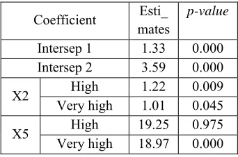
[image:5.612.332.503.376.489.2]After the multicollinearity test is done between the predictor variables on each dataset and overcome if it occurs. Logistic regression modeling was performed between response variables and predictor variables that did not have multicollinearity, then parameter estimation of logistic regression coefficient was done. Partial significance testing of parameters was done to exclude one by one the least significant predictor variables. Next re-modeled the other predictor variables with the response variable, to get the final model is the model with all significant predictor variables. The parameter estimation results from the three datasets for all significant coefficients are presented in the following table:
Table 1: The Estimated Values of the Logistic Legression Parametes for the First dataset
Coefficient Esti_ mates
p-value
Intersep 1 1.33 0.000 Intersep 2 3.59 0.000
X2 High 1.22 0.009
Very high 1.01 0.045
X5 High 19.25 0.975
Very high 18.97 0.000
Based on table 1 above, there are only two predictor variables that have a significant effect on the risk of stroke. Both predictors are X2 and X5. The logistic regression model with significant predictor variables can be written as follows:
Table 2: The Estimated Values of the Logistic Legression Parametes for the Second dataset
Coefficient Estimates p-value
Intersep -11.39 0.000
X9 1.23 0.000
5189 is unfortunate that the majority of the variables suspected to affect the response are not supported by empirical evidence. The logistic regression model with significant predictor variables can be written as follows:
Table 3: The Estimated Values of the Logistic Legression Parametes for the third dataset
Coefficient Estimates p-value
Intersep -11.89 0.000
X3 1.856 0.003
X4 1.241x 10⁻⁵ 0.003
X5 -8.82x 10⁻⁸ 0.039
Based on the above results in the table thirrd, there are three predictors that have a significant effect on the acceptance or rejection of credit application. The variables X3 and X4 have positive coefficients that show the two variables contribute significantly to the probability value of receiving a loan application. While the variable X5 has a negative coefficient which means that the contribution of the variable is relatively small in increasing the probability of receiving the loan application. Logistic regression models with significant predictor variables can be written as follows:
4.2. Modeling SVM
There are two main processes in SVM modeling that are both modeling stage and model implementation stage. Model formation uses data training which includes the steps: a). Normalization of data, b). Mapping input to feature space, c).Estimating kernel function parameters, d). Calculating the Lagrange multiplier value, e). Calculating the bias value. In the implementation phase is done by entering the data testing into the SVM model that has been obtained.
a. Input Data Normalization
Normalization is done by changing the scale of attribute values in the range [0,1]. we haThe first step to normalization is to determine the maximum and minimum values of each attribute of the input data. Suppose that we have both the maximum and minimum values for the attributes of ages are 95 and 23 years respectively. Then we want to change the scale of the attribute age value at the first
observation that is 44 years, the calculation is done in the following way:
The age attribute value at first observation was changed to 0.29167. The same way is done to change all observed values of all other attributes.
b. Mapping Input Data Into Feature Space
Mapping input data into feature space is the most important in solving modeling cases in SVM. To map the data into the feature space is done with the help of the kernel function so that the selection of kernel function parameters is very important. The kernel function used in this paper is Radial Basis Function.
c. Estimating Kernel function parameters
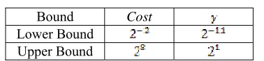
[image:6.612.325.514.426.470.2]Estimation the kernel function parameters are done by gridsearch method. In this method we will try some initial values for the parameter. Here is the initial range of kernel function parameters Radial Basis Function:
Table 4: The Initial Value Range of Kernel Function Parameters.
Bound Cost
Lower Bound Upper Bound
Some values in the range as in Table 4. will be used to find the best parameters. So we get the best parameters for the kernel function as follows:
Table 5: The Best Kernel Function Parameters Parameter Dataset 1 Dataset 2 Dataset 3
Cost 27 2-1 26
2-7 2-5 2-4
The results in Table 5. show the best parameter values obtained through the gridsearch method.
d. Calculating Lagrange Multiplier Value
5190
e. Estimation of bias values (b)
The parameter values of bias b can be estimated by Eq. (13). Here are the estimates values of b for each dataset:
Table 6: The estimates vavues of bias parameters for each dataset
Parameter Dataset 1 Dataset 2 Dataset 3
b 2.948 0.263 0.861
3.705
Based on Table 6. we get b for dataset 1 of 2,948 and 3,705, dataset 2 is 0.263, and dataset 3 is 0.861.
f. Support Vector Machine Classification Model
Based on the calculations presented in the previous session, the SVM classification model for each data can be written as follows:
Dataset 1 :
Dataset 2 :
Dataset 3 :
4.3 Accuracy of Classification in Logistic Regression
Data training is generally used to form models. Before the model is tested on the new data it is necessary to know the level of goodness of the model by calculating the accuracy of the classification in the training data. The precision of classification is used to find out how well the model is derived from predicting the class in the data. Here is the best classification accuracy table on the training data on the logistic regression model that is for the third dataset:
Table 7. Accuracy of Classification for Training Data 3
Class prediction Total Aper Press
’Q
0 1
0 16 3 19
7.46
% 48.49
1 2 46 48
Total 18 49 67
Based on Table 7. it can be observed that there are 16 correct classifications in category 0 ie credit decisions rejected, and there are 3 observations in category 0 misclassified. In addition, there are 46 correct classifications in category 1 namely credit decision accepted, and there are 2 wrong classifications in category 1. The Aper value logistic regression model that is equal to 7.46%, it shows regression model that got good to solve case Classification for lending decisions. In addition, to know the stability in the classification used Press'Q test. Based on the above results, the statistical value of Press'Q test is worth more than = 3.84 so it can be concluded that the classification on data training in dataset third is consistent.
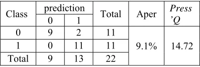
[image:7.612.318.517.371.438.2]The model that has been obtained in the training data will be used for the classification of new data that is data testing. If the model obtained is a good model it will give a small misclassification. Table 8. describes the classification accuracy of the data testing in the third dataset:
Table 8. Accuracy of Classification for Testing Data 3
Class prediction Total Aper Press
’Q
0 1
0 9 2 11
9.1% 14.72
1 0 11 11
Total 9 13 22
Based on Table 8. it can be observed that there are 9 correct classifications in category 0 ie credit decisions rejected, and there are 2 observations in category 0 that are misclassified. In addition, there are as many as 11 correct classifications in
category 1, namely credit decisions
accepted, and there is no classification
errorin category 1. The Aper value logistic regression model that is 9.1%, it shows the regression model obtained is good to resolve cases classification decision Lending. In addition, to know the stability in the classification used Press'Q test. Based on the above results, the statistical value of Press'Q test is worth more than = 3.84 so it is concluded that the classification is consistent.
The overall accuracy of classification results for all datasets for both training and testing data are given in Table 9. below:
Table 9. Accuracy of Classification for Logistic Regressin
5191
Dataset Aper(%) Press’Q Aper(%) Press’Q
1 25.33 115.32 14.00 25.92
2 16.00 34.68 16.00 11.56
3 7.46 48.49 9.10 14.72
When observed more deeply against the results of classification of training data the smallest Aper value occurs in the third dataset that is equal to 7.46%. In all datasets also obtained a statistic press'Q value greater than = 3.84. Similar results also occurred in the data testing, but in general, there was an increase in the value of Aper and decreasing the value of the press'Q statistic. Changes in the value of both Aper and press'Q model accuracy indicators are within reasonable limits.
4.4 Accuracy of Classification in Support Vector Machine (SVM)
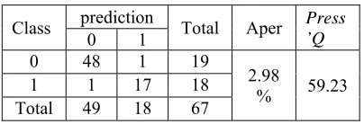
[image:8.612.94.296.477.546.2]The model generated by the SVM method, before being used for the classification of new objects, then must first be calculated the level of accuracy in the training data. Before the model is tested on new data it is necessary to know the goodness of the model by calculating the Aper value and the press'Q statistics. In all three datasets, the model with the best accuracy is the model yielded by the third dataset. The Aper and press'Q values for the SVM model in the third dataset are given in Table 10 below:
Table 10. The SVM Accuracy of Classification of Training Data for Dataset 3
Class prediction Total Aper Press
’Q
0 1
0 48 1 19
2.98
% 59.23
1 1 17 18
Total 49 18 67
Based on Table 10. it can be observed that there are 48 objects classified appropriately in category 0 ie credit decisions rejected, and there is 1object in category 0 misclassified. In addition there are as many as 17 objects that appropriate classification in category 1 is the credit decision is accepted, and there is 1 classification in category 1. Value Aper for SVM method in Data 3 that is 2.98%, it shows SVM classification model that is obtained is good for Solve the classification case of loan decision. In addition, to know the stability in the classification used Press'Q test. Based on the above results the statistic Press'Q is greater than
= 3.84, so it is concluded that the classification is consistent.
Furthermore, the models already obtained in the training data are used for classification in the data testing. Based on the results of this classification will be known how much accuracy of the classification obtained the model. The following is the result of the SVM model in the data testing for the third dataset presented in Table 11:
Table 11. The SVM Accuracy of Classification of Testing Data for Dataset 3
Class prediction Total Aper Press
’Q
0 1
0 13 2 15
9.1% 14.72
1 0 7 7
Total 13 9 22
Based on Table 11. it can be seen that there are 13 objects of exact classification in category 0, and there are 2 objects in category 0 that are misclassified. In addition there are as many as 7 objects that are appropriate classification in category 1, and there is no misclassified object in category 1. Aper value of SVM model in data testing for Dataset 3 is 9.1%, it shows SVM model that got good to finish Case of classification of loan decision. In addition, to know the stability in the classification used Press'Q statistic. Based on the above results the statistic Press'Q is greater than = 3.84, so it is concluded that the classification is consistent.
Summary of the results of the classification of SVM model in both Aper and press'Q statistic for all three datasets are presented in Table 12., the following:
Table 12. Accuracy of Classification for Support Vector Machine Model
Data training Data Testing
Dataset Aper(%) Press’Q Aper(%) Press’Q
1 4.00 265.1 8 77.44
2 8.00 52.92 12 14.40
3 2.98 59.23 9.1 14.72
5192
4.5 The Comparison of both logistic regression and SVM classification models
The classification accuracy as measured by Aper values from logistic regression models and SVM models in training and testing data for all three datasets is presented in Table 13. Follows:
Table 13. The Value Aper (%) for Logistic regression model and SVM
Data training Data Testing
Dataset Log. Reg. SVM Log. Reg. SVM
1 25.33 4.00 14.00 8.00
2 16.00 8.00 16.00 12.00
3 7.46 2.98 9.10 9.10
As a resume, the accuracy of SVM classification is better than the accuracy of logistic regression in both training and testing data. This is indicated by the smaller Aper values obtained on the SVM model. The accuracy of the classification of training data for logistic regression has a high diversity, even in the first dataset with the characteristics of all continuous-scale predictor variables, Aper value equal to 25.33%. However, the Aper value on the same dataset for the SVM model is only 4%. It implies that with all predictor variables of the continuous type the logistic regression model generated is less able to classify the object well, whereas the contradiction situation occurs in the SVM model. In the second dataset that has characteristic all predictor variables of categorical type result of relatively equal Aper value for both models, either accuracy in training or testing data. Although the Aper value for the SVM model in the second dataset is also smaller than the Aper value of the logistic regression model. In the third dataset with predictor variables of mixed type between numerical and categorical, both models of logistic regression and SVM are obtained with very high accuracy in both training and testing data.
5. CONCLUSIONS
Based on the presentation given in the previous session, the following conclusions can be drawn:
1. In the training data, the performance of the SVM model classification is signicantly better than the logistic regression model classification.
2. In the testing data, the performance both logistic regression models and SVM
models have satisfactory classification Aper values, although the Aper value of the svm model is rather convincingly smaller.
3. The results of this study further reinforce the existing paradigm, namely that the SVM model is more powerful in the categorization of objects than logistic regression model.
REFRENCES:
[1]
Press, S.J., and Wilson, S. "Choosing between logistic regression and discriminant analysis."
Journal of the American Statistical
Association 73.364 (1978): 699-705..
[2] Dreiseitl, S., and Ohno-Machado, L. "Logistic regression and artificial neural network classification models: a methodology review."
Journal of biomedical informatics 35.5 (2002):
352-359.
[3] Felicísimo, Á.M., et al. "Mapping landslide susceptibility with logistic regression, multiple adaptive regression splines, classification and regression trees, and maximum entropy methods: a comparative study." Landslides 10.2
(2013): 175-189.
[4] Maulidya. The Comparison of Discriminant
Analysis and Logistic Regression. Thesis,
Faculty of Sciences , University of Brawijaya, Malang. 2013.
[5] Burges, C. "A tutorial on support vector machines for pattern recognition." Data mining
and knowledge discovery 2.2 (1998): 121-167.
[6] Smola, A.J, and Schoelkopf, B. A tutorial on
support vector regression: Tech. Rep.
NeuroCOLT2 NC2-TR-1998-030: 1998. http://citeseer. ist. psu. edu/smola98tutorial. html, 1998.
[7] Herbrich, R., Graepel,T., and Obermayer, K.
Large margin rank boundaries for ordinal
regression. MIT Press Cambridge. 2000.
[8] Hastie, T., and Tibshirani, R. "Classification by pairwise coupling." Advances in neural
information processing systems. 1998.
[9] Schölkopf, B. and Smola, A.J. Learning with kernels: support vector machines,
regularization, optimization, and beyond. MIT
press, 2002.
5193
of the eleventh ACM SIGKDD international conference on Knowledge discovery in data
mining. ACM, 2005.
[11] Akbar, A.L. The Implementation of Support Vector Machine algorithm to determine the risk
of stroke. Thesis. Faculty of Computer Sciences,
university of Brawijaya, Malang.. 2015.
[12] Utama, M.P. Analysis of Factors Affecting Decision Granting of People's Business Credit..
Thesis, Faculty of Sciences , University of Brawijaya, Malang . 2012 .
[13] Hosmer, David W., and Stanley Lemeshow.
Special topics. John Wiley & Sons, Inc., 2000.
[14] Bishop, C. M. Pattern recognition and machine
learning. springer, 2006.
[15] Vapnik, Vladimir N. "Statistical learning theory. Adaptive and learning systems for signal processing, communications, and control." (1998).