Munich Personal RePEc Archive
Tariff and Equilibrium Indeterminacy–A
Note
Zhang, Yan and Chen, Yan
New York University, Shandong University
12 June 2008
Online at
https://mpra.ub.uni-muenchen.de/10044/
Tari¤ and Equilibrium Indeterminacy–A Note
Chen Yan
Center for Economic Research, Shandong University
Yan Zhang
Department of Economics, New York University,
269 Mercer Street, 7th Floor, New York, 10003, USA
June 12, 2008
Abstract
We explore the equivalence between the factor income taxes (in Schmitt-Grohe
and Uribe 1997) in the closed economy and the tari¤ in the open economy, in the
sense that they share similar propagation mechanism of sunspot and fundamental
shocks under a balanced-budget rule.
Key Words: Sunspots, Endogenous Tari¤ Rate, Comovement
JEL Classi…cation Number: F41, Q43
1. Introduction
It has been known that indeterminacy may arise as a consequence of complicated
gov-ernment policies that allow for feedback from the private sector to future values of …scal
policy variables. A class of models of …scal increasing returns includes Blanchard and
Summers (1987) and Schmitt-Grohe and Uribe (1997, in short SGU). The key to
gener-ate indeterminacy in those models is that keeping the government expenditure constant,
an increase in the capital stock can expand the tax base and reduce the tax rate. The
after tax return of the capitalmay increase as the capital stock increases, therefore the
original rise in the shadow price of capital needs to be reversed and the system moves
back towards the steady state, generating another equilibrium path.
Tari¤ as a source of …scal increasing returns may share a similar channel with the
factor income taxes to generate indeterminacy, see Zhang (2008). In Zhang, we …nd
that if the government needs to …nance its pre-set level expenditure through imposing
a tari¤ on imported oil, it will make the endogenous rate to be countercyclical with
respect to the output, thus a similar mechanism occurs.
In this paper, we introduce intrinsic uncertainty in the form of exogenous
produc-tivity and government purchases shocks and investigate the propagation mechanism of
sunspot and fundamental shocks under a balanced-budget rule in the tari¤ model. SGU
conduct a calibration of their model and observe the comovements of the variables
results, thus validating the notion that tari¤s and factor income taxes are equivalent.
2. The One-Sector Open Economy With Tari¤ Revenue
This is the one-sector oil-in the production RBC model studied by Zhang (2008). A
representative agent maximizes the intertemporal utility function
E0
1
X
t=0
t(logc
t bnt) (1)
wherectis consumption of a single good which is the numeraire and tradeable, nt labor
supply and 2(0;1)is the subjective discount rate in the discrete time model. Assume
that the economy is open to importing oil so that the agent can use the tradeable good
to buy oil. The oil price is assumed to be exogenous and its supply from the rest of the
world is assumed to be perfectly elastic.
On the production side, there is a single good produced with a Cobb-Douglas
produc-tion technology with three inputs–capital (kt), labor (nt) and non-reproducible natural
resources (ot)1 :
yt=ztkatkn an
t o a0
t (2)
where the third factor in the production, non-reproducible natural resources, say oil (ot),
is imported, and the technology displays the constant returns to scale (ak+an+a0 = 1).
Assuming the …rms are price takers in the factor markets, the pro…ts of the …rms are
given by
=y (r+ )k wn po(1 + )o (3)
where (r+ ) denotes the user cost of renting capital2, w denotes the real wage, and
po denotes the real price of oil (the imported goods). is the (endogenous) tari¤ rate
imposed on the imported oil, which is uniform to all …rms. Perfect competition in factor
and product markets implies that factor demands are given by:
wt=an
yt
nt
rt+ =ak
yt
kt
po(1 + t) =a0
yt
ot
Since we assume that the foreign input is perfectly elastically supplied, the factor
price, po, is independent of the factor demand for o, we can obtain the reduced form
production function as we substitute outot=a0po(1+yt
t) in the equation (2),
yt=ztAk
ak
1 a0
t n
an
1 a0
t 3. (4)
The government collects the tari¤ revenue to …nance its pre-set level expenditure
as in SGU.
po tot=G
The agent budget constraint is
ct+st+1= (1 +rt)st+wtnt+ t
where st is aggregate saving4. Here the aggregate factor payment, po(1 + t)ot goes
to the foreigners (poo
t) and the government (po tot). The …rst order conditions with
respect to labor supply and savings are given by
b = wt
ct
1 ct
= Et
1 ct+1
(1 +rt+1)
4We assume that the government consumes the tari¤ revenue from the importing oil. G=po tot=
ta0yt
In equilibrium, st=kt, and factor prices equal marginal products5.
As we see in Zhang (2008), the number of the tari¤ rates that generate enough
revenue to …nance a given level of government revenue can be 0, 1 or 2. As the steady
state tari¤ rate is in an open interval, the indeterminacy appears.6
We analyze the solution to a log-linear approximation of the equilibrium conditions
of the model, which, in addition to sunspot shocks, is also subject to technology and
government purchases shocks. When the equilibrium is indeterminate, the equilibrium
conditions can be reduced to the following …rst-order stochastic linear di¤erence
equa-tion: 2 6 6 6 6 6 6 6 6 6 6 4 bt+1 b kt+1 b zt+1 gt+1 3 7 7 7 7 7 7 7 7 7 7 5 = 2 6 6 4
M Mf
0 3 7 7 5 2 6 6 6 6 6 6 6 6 6 6 4 bt b kt b zt gt 3 7 7 7 7 7 7 7 7 7 7 5 + 2 6 6 6 6 6 6 6 6 6 6 4
"st+1
0
"z t+1
"gt+1
3 7 7 7 7 7 7 7 7 7 7 5 (5)
where is a 2 2 diagonal matrix and M is a 2 2 matrix with both eigenvalues
inside the unit circle.7The diagonal (
z; g) in denotes the serial correlation of the
5The …rst order conditions, budget constraint of the household and the government balanced budget
requirement become: bnt = 1
ctanyt, 1
ct = Et
(1 +akyt+1
kt+1)
ct+1 , ct+kt+1 = (1 )kt+ (1 a0)yt, and po tot=G.
6The upper and lower bounds of the interval are determined by the system parameters. 7The matrix [
exogenous processes for productivity,zt, and government expenditures, gt, respectively.
We assume that the productivity and the government expenditures innovations,"zt and
"gt, have mean zeros and are serially uncorrelated and orthogonal to each other. The
sunspot innovation "st is assumed to have zero mean and be serially uncorrelated but
potentially contemporaneously correlated with either of the fundamental innovations.8
All variables in (5) are expressed as percentage deviations from the steady state.
For the calibration of our model, we assume that the time unit is a quarter, the
steady state tari¤ rate of oil in this country is 60 percent, and the serial correlation of
both fundamental shocks is 0.9 ( z = g).9 The remaining parameters take the values
as in Wen and Aguiar-Conraria (2005)10. Given the above values of those parameters,
the rational expectation equilibrium is indeterminate.
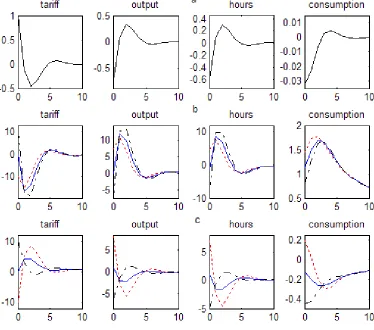
Figure 1 displays the impulse responses of the tari¤ rate, output, hours, and
con-sumption to sunspot ("s0 = 1), technology ("z0 = 1), and government expenditures shocks
("g0 = 1). Panel a of …gure 1 shows the impulse responses to one unit innovation ("s 0 = 1)
in the tari¤ rate under the assumption that "s
t is uncorrelated with any fundamental
shock. The initial increase in the tari¤ rate triggers a highly persistent, hump-shaped
response in aggregate economy variables and tari¤ rate. When the equilibrium is
in-determinate, the initial responses of endogenous variables to fundamental shocks is
8In our numerical exercise,"s
t+1=bt+1 Et[bt+1]can be viewed as the forecast error ofbt+1 9The steady state tari¤ rate is the optimal rate calculated by Newbery (2005), which is consistent
with the one in EU (2002). See Zhang (2008).
not necessarily magni…ed. Panels b and c of …gure 1 show, respectively, the impulse
responses to technology and government expenditure shocks under three alternative
as-sumptions about the initial percentage deviations in the tari¤ rate: 10,0, and 10. As
shown in panel b, for example, a positive innovation in the technology shock can lead
to a contraction in output if the initial response of the tari¤ rate is su¢ciently above
the steady state. Under indeterminacy, the impulse responses of aggregate economy
variables are highly persistent, hump-shaped regardless of the the initial value of the
tari¤ rate.
When the economy is subject to fundamental and sunspot shocks, the comovements
of tari¤s, output, hours, and consumption depend in principle on our assumed
correla-tion of the sunspot shock with the fundamental shock and on the relative importance of
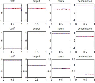
each source of uncertainty. Figure 2 summarizes this relationship when the only sources
of uncertainty are sunspot shocks and persistent productivity shock ( a= 0:9). It shows
the serial correlation (panel a), the contemporaneous correlation with output (panel b),
and the standard deviation relative to output (panel c) of the tari¤ rate, output, hours,
and consumption as a function of the variance of sunspot shock, 2
"s. For three di¤erent
values of the correlation between the sunspot and the technology shocks: 1,0, and 1,
the variance of the sunspot shock, 2
"s, is shown on the horizontal axis; it takes values
between zero and one. The variance of innovation in the technology shock, 2"z, is set
is equal to one, 2
"s + 2"z = 1. The …gure 2 encompasses two extreme cases: one in
which the economy is hit only by sunspot shocks ( 2"s = 1, 2"z = 0) and another in
which the economy is hit only by technology shock( 2"s = 0, 2"z = 1). Each plot
dis-plays three lines: the solid line corresponds to the case in which the sunspot and the
technology innovations are uncorrelated (corr("s
t; "zt) = 0), a dotted line corresponds to
the case in which the correlation between the sunspot and the technology innovations
is equal to 1 (corr("s
t; "zt) = 1), and a chain-dotted line corresponds to the case in
which the correlation between the sunspot and the technology innovations is equal to
1 (corr("s
t; "zt) = 1). Panel a, b, and c show, respectively, the …rst-order correlation,
the contemporaneous correlation with output, and the standard deviation relative to
output of the tari¤ rate, output, hours, and consumption as a function of the variance
of the sunspot shock ( 2"s).
The main implication of …gure 2 is that neither the …rst-order serial correlations,
the contemporaneous correlations with output, nor the standard deviation relative to
output of tari¤ rates, hours, and consumption is a¤ected by the relative volatility of
the sunspot shock or its correlation with the technology shock. This can be seen in the
fact that in most cases the three lines are perfectly ‡at and indistinguishable from each
other. This shows that rational expectations equilibrium under the indeterminacy case
does not necessarily imply that any arbitrary pattern of comovement in endogeneous
joint distribution of sunspot and fundamental shocks11.
References
[1] Blanchard, O.J. and L.H. Summers, 1987. Fiscal Increasing Returns, Hysteresis,
Real Wages and Unemployment, European Economic Review 31, 543-559.
[2] Newbery, D., 2005, Why Tax Energy? Towards a More Rational Policy, The Energy
Journal, Vol.26, No.3
[3] Stephanie Schmitt-Grohe, Martin Uribe, Balanced-Budget Rules, Distortionary
Taxes, and Aggregate Instability. Journal of Political Economy, October 1997, 105,
976-1000
[4] Wen, Yi, Luis Aguiar-Conraria, Foreign trade and equilibrium indeterminacy,
Fed-eral Reserve bank of St. Louis, 2005-041a
[5] Zhang, Yan, 2008a, Tari¤ and Equilibrium Indeterminacy–(I), PhD thesis, Dept. of
Economics, New York University
1 1When the economy is subject to persistent government expenditure and sunspot shocks, a similar
Figure 2.1: —Impulse responses. a, Sunspot shock, "s
0 = 1. b, Technology shock, "z0 = 1. c,
Figure 2.2: —–Comovements. Each plot shows either the serial correlation (panel a), the contemporaneous correlation with output (panel b), or the standard deviation relative to output (panel c) as a function of the variance of sunspot shock, 2"s, for three di¤erent values of the correlation between the sunspot and the technology shocks: 1, 0, and 1. The variance of the sunspot shock, 2"s, is shown on the horizontal axis; it takes values between zero and one. The variance of innovation in the technology shock, 2"z, is set so that the sum of the variance of the innovations in the technology and sunspot shocks is equal to one, 2"s + 2"z = 1. —
corr("s