Demand for meat quantitu and quality in Malaysia: Implications to Australia

(1)

Munich Personal RePEc Archive

Demand for meat quantitu and quality in

Malaysia: Implications to Australia

Tey, (John) Yeong-Sheng and Mohamed Arshad, Fatimah

and Shamsudin, Mad Nasir and Mohamed, Zainalabidin and

Radam, Alias

8 September 2008

Online at

https://mpra.ub.uni-muenchen.de/15032/

(2)

DEMAND FOR MEAT QUANTITY AND QUALITY IN MALAYSIA: IMPLICATIONS TO AUSTRALIA

by

Tey (John) Yeong-Sheng*1, Fatimah Mohamed Arshad1, Mad Nasir Shamsudin2, Zainalabidin Mohamed3, and Alias Radam1

Abstract

As per capita income increases, consumers do not only demand for a greater quantity but also higher quality of food. The objective of this study is to examine the demand for meat quantity and quality in Malaysia. By using the Household Expenditure Survey 2004/05 data, expenditure, quantity, and quality expenditures are obtained via Engel curves analyses. The empirical results show that Malaysians are increasingly demanding for quality meat products. To be more specific, urban consumers are more likely to spend on higher quality meat products than rural consumers. By understanding and reacting to the changes in demand for meat products in Malaysia, Australia can offer the right range of meat products earlier than other competitors while continue enjoying their market leadership in the niche of quality meat segments.

Keywords: Engel curves, Meat, Quantity, Quality

JEL code: D12

1.0 Introduction

The changes in Malaysian food consumption pattern can be characterized by the decreasing per capita consumption of staple food-rice and increasing per capita consumption of wheat, meats, fish, vegetables, and fruits. Such changes balance off the need of multi-nutrition rather than meeting basic calorie need in Malaysian diet. Economists attribute these changes mainly to income growth and rural-urban migration that bring emergence in lifestyle and diet. The income effect was measured by Tey et al.

(2008a) recently. Tey et al. (2008a) found that expenditure elasticities for meat, fish, vegetables, and fruits are 1.11, 0.910, 1.341, and vegetables respectively. The elasticities suggested that Malaysian consumers tend to consume more meat as income increases.

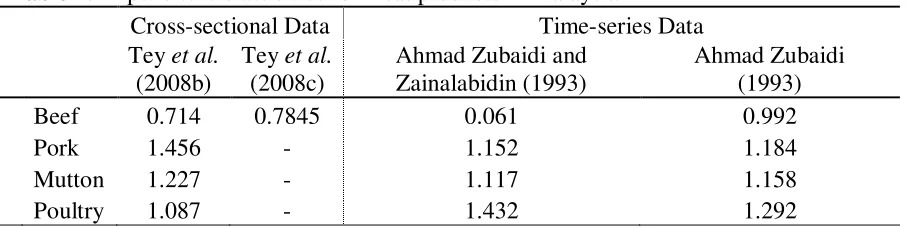
Specifically, Table 1 presents the expenditure elasticities for individual meat products obtained from previous studies. By using the Household Expenditure Survey (HES) 2004/05 data, Tey et al. (2008b) found that expenditure elasticities for beef, pork, mutton, and poultry are 0.714, 1.456, 1.227, and 1.087 respectively. Similar expenditure elasticities were found in Ahmad Zubaidi and Zainalabidin (1993) and Ahmad Zubaidi

1

Institute of Agricultural and Food Policy Studies, Universiti Putra Malaysia, Malaysia.

* Corresponding author: [email protected]

2

Faculty of Environmental Studies, Universiti Putra Malaysia, Malaysia. 3

(3)

[image:3.612.85.538.133.247.2]

(1993) that used time-series data. The analyses on cross-sectional and time-series data obtained inelastic expenditure elasticities for beef suggested that beef is a normal good; elastic expenditure elasticities for pork, mutton, and poultry suggested that pork, mutton, and poultry are luxury goods in Malaysia.

Table 1: Expenditure elasticities for meat products in Malaysia

Cross-sectional Data Time-series Data Tey et al.

(2008b)

Tey et al.

(2008c)

Ahmad Zubaidi and Zainalabidin (1993)

Ahmad Zubaidi (1993) Beef 0.714 0.7845 0.061 0.992

Pork 1.456 - 1.152 1.184

Mutton 1.227 - 1.117 1.158 Poultry 1.087 - 1.432 1.292

However, the expenditure elasticities that suggested beef is a normal good is questionable, in spite of the fact that beef is one of the most expensive food products in Malaysia. Averagely, it was priced at RM15.46/kg for local and imported beef and RM7.97 for Indian beef compared to RM5.37/kg of poultry in 2005 (Department of Veterinary Services, 2008). Therefore, there could be a change in beef demand, in terms of quantity or quality. A recent study by Tey et al. (2008c) found that Malaysian consumers prefer quantity over quality in demand for beef though they are willing to pay for more expensive beef products. The shortfall of this study is that it used aggregated beef data but beef meat is mainly sold in two forms, fresh/chilled and frozen in Malaysia.

Per capita consumption of poultry is seen that they have reached a saturation point in quantity consumed in recent years. This is because the demand for quantity diminishes as income rises. In other words, as income increases, consumers do not only demand for a greater quantity but also higher quality of food. Hence, this study intends to examine the demand for meat quantity and quality in Malaysia. Identifying these changes in demand form has been of great interest to domestic and foreign meat producers in developing marketing strategies for major meat products, namely beef, pork, mutton, and poultry.

2.0 Meat Consumptions and Self-sufficiency Levels in Malaysia

Figure 1 presents the annual per capita beef, pork, poultry, and mutton consumption in Malaysia, 1960-2005. It can be observed that there are two main characteristics of meat consumption in Malaysia over the last four decades. One is the per capita consumption of poultry and pork that have reached a saturation point. Per capita consumption of poultry and pork had increased steadily since 1960 and reached the peak in 1990s. Per capita consumption of poultry and pork was 3.46kg and 14.43kg in 1960 and 34.3kg and 7.67kg in 2005 respectively. The popularity of poultry was made possible by the large production that saw the price of poultry cheapest amongst all the meat products.

(4)

[image:4.612.112.500.105.314.2]

consumption of beef and mutton has increased from 1.56kg and 2.25kg in 1960 to 5.5kg and 0.75kg respectively in 2005 respectively.

Figure 1: Annual per capita consumption of meats in Malaysia, 1960-2005

0 5 10 15 20 25 30 35 40

Yea r

1963 1966 1969 1972 1975 1978 1981 1984 1987 1990 1993 1996 1999 2002

k

g

/y

e

a

r

Beef Mutton Pork Poultry

Source: Food and Agriculture Organization of the United Nations, 2007.

[image:4.612.86.528.516.596.2]

Figure 2 presents annual self-sufficiency levels of beef, pork, mutton, and poultry in Malaysia, 1960-2005. Though production of beef and mutton has grown steadily from 17.5 metric tonnes and 0.9 metric tonnes in 2000 to 28.5 metric tonnes and 1.5 metric tonnes in 2005 and is expected to produce 45 metric tonnes and 2.3 metric tonnes in 2010 respectively, self-sufficiency level of beef and mutton only managed to grow from 15 per cent and 6 per cent in 2000 to 23 per cent and 8 per cent in 2005 and is expected to attain 28 per cent and 10 per cent in 2010 respectively. Such low self-sufficiency level in beef and mutton has forced the country to rely on imports to meet the increasing domestic demand. While per capita consumption of poultry and pork has met saturation point, it is clear that Malaysia has been fully self-sufficient in these two meat products.

Table 2: Annual self-sufficiency levels (%) of meats in Malaysia

2000 2005 2010

Beef 15 23 28

Pork 100 107 132

Mutton 6 8 10

Poultry 113 121 122

Source: Ninth Malaysian Plan.

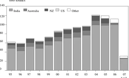
3.0 Meat Import Market in Malaysia

Since Malaysia is not self-sufficient in beef, imports are the answer to domestic demand. Beef imports in Malaysia have increased from 1,955 tonnes in 1970 to 104,140 tonnes in 2006 (Department of Veterinary Services, 2008). Figure 2 presents Malaysia beef imports from various countries during the period of 1995-2007. Before 2006, India, New Zealand, and Australia were the largest suppliers to Malaysia. However, failure to comply with

(5)

Malaysian beef market since 2005. Similarly, Australian beef was also once halted from entering Malaysia during the same period. But the ban was soon retracted in 2006. Therefore, it can be observed that now Malaysian beef imports are dominated by Indian beef. Malaysia imported around 100,000 tonnes of Indian beef in 2006, 36 per cent more than in 2002 (Drum and Gunning-trant, 2008).

However, the imported Indian beef is rather low quality buffalo meat, which means that the market of premium beef is still wide open to foreign producers. The major sources of premium beef imports to Malaysia are Australia, New Zealand, United States, China, Indonesia, Uruguay, and Argentina. A strong gain in the Australian dollar against the Malaysian Ringgit has made beef imports from Australia more costly in recent years. Coupled with Malaysian government policy to open beef market to more halal foreign producers, it is observed that a shrink in Australian beef imports has seen an increase in beef imports from other countries that include China, Indonesia, Uruguay, and Argentina at the same time since 2005. While the demand for beef in Malaysia is expected to continue to grow in the future, a declining market share in a major and growing market is a serious challenge for the Australian beef industry.

Source: Meat & Livestock Australia, 2008.

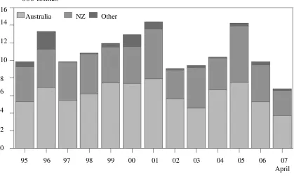
Malaysia is a net importer of mutton. Figure 3 presents Malaysia mutton imports from 1995 to 2007. Obviously, Australia has dominated the mutton imports, followed by New Zealand during the same period. However, both Australian and New Zealand mutton imports have experienced declining trend after 2005. It was because of the similar halal

issue experience by beef industry as well as currency exchange rate effect.

95 96 97 98 99 00 01 02 03 04 05 06 07 April 140

‘000 tonnes

100 120

60 80

20 40

0

Note: Other include China, Indonesia, Uruguay and Argentina

Australia

[image:5.612.98.517.327.581.2]

India NZ US Other

(6)

Source: Meat & Livestock Australia, 2008

4.0 Methodology

4.1 Theoretical Framework

Ordinary Engel curve explains that the change of expenditure for different goods is a function of income, while holding prices fixed. In the simplest form, the Engel curve can be expressed as:

) ( )

(y pq y

e_i  _i _i (1)

where e_i is per capita expenditure on ith food item, y is per capita income, p_i is the price of ith food item, and q_i is quantity purchased of ith food item. The Engel curve is useful to capture empirical consumption behaviors by estimating expenditure elasticities. While price is assumed to be independent of y, if expenditure elasticity, e_i'(y)0 implies that

ith food item is a normal good should also seeq_i'(y)0. In other words, the expenditure and quantity elasticities with respect to y are equal.

While having these variables underlying the Engel curve, an increase in expenditures on

ith food item may be due to increase in quantity purchased or increase in price paid or both. The willingness to pay for higher price implies a shift toward higher quality ith food item. Hence, price data is an indication of food quality. The quality effect, v_i'(y), can then be incorporated in Equation 1 and expressed as:

) ( ) ( )

(y v y q y

ei  i i (2)

95 96 97 98 99 00 01 02 03 04 05 06 07 April Australia NZ Other

Note: Other include India

0 2 4 6 8 10 12 14 16

[image:6.612.97.516.82.334.2]

‘000 tonnes

(7)

Quality elasticity, v_i'(y)0, if consumers purchase ith food item with higher price when their incomes increase. Therefore, the expenditure elasticity, _i, is the sum of the quality elasticity, _i, and the quantity elasticity, _i:

i i

i  

   (3)

4.2 Model Specification

The ordinary Engel curve is a linear form. Recent study by Tey (2008d) found non-linear patterns in Engel curves estimated for consumers in Malaysia. The importance of non-linearities in Engel curve was well emphasized by Blans et al. (1999). This study adopts similar Engel curves analysis technique that has been widely used by Sarma et al. (1979), Alderman and Garcia (1993), Douglas and Isherwood (1996), and Gale and Huang (2007) in determining the demand for quantity and quality of foods.

A quantity-Engel equation can be expressed as:

ij j j i j i i

ij y y D u

q )  (1/ ) log( ) 

log(    (4)

where qijis per capita quantity of the ith meat product consumed by the jth household, j

y is the per capita income of the jth household, D is a set of demographic variables (household size, employment status, urban region, race, age and gender of respondent), and u_ij is a random disturbance term. From Equation 4, quantity elasticity of the ith meat product, _i, can be estimated by:

i j i

i  y 

  /  (5)

An expenditure-Engel equation can be expressed as:

ij j j i j i i

ij y y D u

e ) * *(1/ ) *log( ) 

log(    (6)

where e_ij is per capita expenditure of the ith meat product by the jth household, and other variables are same like those described earlier. From Equation 6, expenditure elasticity of the ith meat product, _i, can be obtained by:

* /

* _i

i

i  y 

   (7)

Followed Equation 3, after obtaining quantity elasticity, _i, and expenditure elasticity, _i, quality elasticity, _i, can be estimated by:

i i

i  

   (8)

4.3 Estimation Technique and Data

This study utilizes data from the Malaysian Household Expenditure Survey (HES) 2004/05. The data consists of 14,084 sample size, where data of 9,467 and 4,617 respondents was collected in urban and rural regions respectively. In this study, the Engel equations are estimated for a more comprehensive and detailed breakdown of meat categories on three bases, namely nationwide, urban and rural regions. This is because there have been many structural changes in Malaysian food landscape in recent years, including the rise of income levels and rapid development of supermarkets and hypermarkets in urban regions that both see expansion of affordability for and availability of higher quality food products.

(8)

Equations (4) and (6) can be estimated using ordinary least squares estimator (OLS). However, the HES 2004/05 data was collected from different states with different number of households surveyed over different months. This may present heteroskedasticity in the data. Thus, White heteroskedasticity tests (with cross terms) were conducted and detected the presence of heteroskedasticity. In order to handle the presence of heteroskedasticity, the Engel equations were estimated using Weighted Least Squares procedure.

5.0 Empirical Results

Appendix tables 1, 2, 3, 4, 5, and 6 present the regression results of expenditure and quantity Engel equations for urban, rural, and Malaysia (total) respectively. Both the _i and _i parameters are statistically significant in all the equations. It is noteworthy that there are consistent negative relationships between expenditures and quantity on meat products and household size in all cases due to the economies of scale enjoyed as household size expands. The estimates of age are positive and significant in most cases, except in frozen pork and frozen mutton. The positive estimates indicate that older consumers spent and consumed more meat products than younger consumer. There are variation of significance level and sign in the cases of gender, employment status, and ethnic.

[image:8.612.87.527.517.677.2]

Table 3 presents the quantity elasticity of meat products in Malaysia. In general, all expenditure elasticities are less than 1 for all meat products. This shows that all the meat products are normal goods to Malaysians. To be more specific, the magnitudes of expenditure elasticities in rural are higher than urban regions. In rural regions, expenditure elasticities for meat products range from 0.3373 to 1.3359; in urban regions, expenditure elasticities for meat products range from 0.0127 to 0.3616. These suggest that rural consumers are more likely to increase their expenditures on meat products than urban consumers as their incomes rise. Rural consumers tend to increase their expenditures on luxury goods-fresh/chilled mutton (1.2016) and frozen mutton (1.3359) faster than other meat products.

Table 3: Expenditure elasticity of meat products

Expenditure Elasticities

Urban Rural Total

Fresh/chilled beef 0.2730 0.4425 0.3114 Fresh/chilled pork 0.2787 0.6451 0.3098 Fresh/chilled mutton 0.3616 1.2016 0.3745 Fresh/chilled Poultry 0.2481 0.3373 0.2684 Frozen beef 0.3302 0.4508 0.3526 Frozen pork 0.1331 0.7380 0.3777 Frozen mutton 0.0127 1.3359 0.1890 Frozen poultry 0.2006 0.4327 0.2588

(9)

consumers are approaching or have approached saturation levels of quantity consumed for meat products, except fresh/chilled beef and frozen beef. For example, quantity elasticities of the frozen mutton (3.4707) and frozen pork (2.5215) are relatively high for rural consumer, but diminish rapidly to -1.0793 and 0.0266 respectively as they move to urban. Quantity elasticities for poultry-which account for most meats consumed by Malaysians-are close to zero at all levels.

[image:9.612.87.528.273.435.2]

The quantity elasticities for fresh/chilled pork and frozen mutton show a puzzling pattern for urban as well as Malaysian consumers as a whole. The estimated quantity elasticities for fresh/chilled pork are positive in rural regions (0.5993) and become negative in urban regions (-0.1049). In rural regions, frozen mutton has the highest quantity elasticity (3.4707) but becomes the smallest quantity elasticity (-1.0793) in urban regions. These mystifying patterns are likely a clue that shows urban consumers tend to substitute quality over quantity of meat products.

Table 4: Quantity elasticity of meat products

Quantity Elasticities

Fresh/chilled beef 0.1176 0.4916 0.1827 Fresh/chilled pork -0.1049 0.5993 -0.1082 Fresh/chilled mutton 0.0442 2.2466 0.2438 Fresh/chilled Poultry 0.0260 0.0405 0.0241 Frozen beef 0.1776 0.6607 0.2837 Frozen pork 0.0266 2.5215 0.4631 Frozen mutton -1.0793 3.4707 -0.5553 Frozen poultry 0.0178 0.4272 0.0848

Table 5 presents the quality elasticity of meat products in Malaysia. Overall, most expenditure elasticities are larger in magnitude than the corresponding quantity elasticities. In other words, expenditures on most meat products are expected to rise faster than the quantity purchased in response to income growth. The difference is indeed a reflection of quality effect. In total, quality elasticities are less than 1 and only the sign of frozen pork is negative. In particular, positive quality elasticities are found in urban regions while there are variations of sign across the meat products in rural regions. This suggests that consumers are increasingly seeking quality meat products as they move from rural to urban regions.

Special attention is paid to the case of poultry in order to explain why per capita consumption has reached saturation points. Poultry is indeed the cheapest meat product in Malaysia, where it is homogeneous product to all ethnics in Malaysia. Taking urban-rural estimates into consideration, the expenditure elasticities for poultry range from 0.2006 to 0.4327 are greater than quantity elasticities that range from 0.0178 and 0.4272. Though both expenditures and quantity purchased rise with income, the difference indicates that expenditures are expected to rise faster than quantity purchased of poultry.

(10)

[image:10.612.86.539.191.351.2]

respectively. Such puzzling patterns suggest that urban consumers are more likely to demand for quality higher value meat products-beef and mutton than rural consumers, which could be mainly attributed to income and urbanization effects. Income levels in urban regions are generally higher than rural regions. Consequently, urban consumers have stronger buying power for the quality higher value meat products. The buying power is realized with actual purchase that is made possible by availabilities of imported beef and mutton, which are obviously perceived as higher quality meat products than local bred, at super- and hypermarkets in urban regions.

Table 5: Quality elasticity of meat products

Quality Elasticities

Fresh/chilled beef 0.1553 -0.0491 0.1287 Fresh/chilled pork 0.3837 0.0457 0.4180 Fresh/chilled mutton 0.3174 -1.0451 0.1307 Fresh/chilled Poultry 0.2221 0.2968 0.2443 Frozen beef 0.1527 -0.2099 0.0690 Frozen pork 0.1065 -1.7835 -0.0854 Frozen mutton 1.0920 -2.1348 0.7444 Frozen poultry 0.1828 0.0055 0.1740

6.0 Policy Implications

Since Malaysian has not been self-sufficient in beef and mutton, the growing demand for both quantity and quality indeed signals a growing market and a tendency to become a mature market for meat products. However, the market has become more competitive with its open policy to welcome more halal foreign producers in order to make the higher value meat products more affordable to Malaysian consumers. In this sense, not only does Australia have to comply and sustain the halal requirements, but also to supply both quantity and quality of beef to Malaysia at economical pattern.

While facing these challenges, Australia is also to determine whether to protect and capitalize their long-enjoyed competitive advantage in the Malaysian market. Competing in a growing market that is postulated to become a mature market, country-of-origin marketing strategies are no longer enough to form a complete sense of trustworthy and preference. This is crucial as the consumers are better educated and increasingly quality conscious. Responding to the changing consumers’ preferences is the key determinant in capturing market share and become market leader in quality beef and mutton segments via more dynamic marketing mix.

7.0 Conclusions

(11)

quantity of all meat products diminishes as consumers move from rural to urban regions. The differences between the expenditure and quantity elasticities suggest that additional meat expenditures by urban consumers are more likely to be spent on higher quality meat products. By understanding and reacting to the changes in demand for meat products in Malaysia, Australia can offer the right range of meat products earlier than other competitors while continue enjoying their market leadership in the niche of quality meat segments.

References

Ahmad Zubaidi, B. 1993, ‘Applying the almost ideal demand system to meat expenditure data: Estimation and specification issues. Malaysian Journal of Agricultural Economics, vol. 10.

Ahmad Zubaidi, B. and Zainalabidin, M. 1993, ‘Demand for meat in Malaysia: An application of the almost ideal demand system analysis, Pertanika Social Science and & Humanities, vol 1, no. 1, pp. 91 – 95.

Alderman, H. and Garcia, M. 1993, Poverty, household food security, and nutrition in rural Pakistan, International Food Policy Research Institute, Research report: No. 96.

Department of Veterinary Services. 2008. Livestock Statistics. [Online]. Available at:

http://agrolink.moa.my/jph/dvs/statistics/statidx.html [accessed 1 August 2008]

Douglas, M. and Isherwood, B. 1996. The World of Goods: Towards an Anthropology of Consumption. (2nd ed.). Routledge, London.

Drum, F.and Gunning-Trant, C. 2008, ‘Live animal exports: A profile of the Australian industry’, ABARE research report 08 for the Australian Government Department of Agriculture, Fisheries and Forestry, Canberra, February.

Gale, F. and Huang, K. 2007, Demand for food quantity and quality in China, Economic Research Service, United States Department of Agriculture, Economic Research Report Number 32.

Meat and Livestock Market Statistics. 2008. Meat & Livestock Australia. [Online].,

available at:

http://marketdata.mla.com.au/default.asp?RegionID=6&CategoryID=46&Classifi

cationID=66 [accessed 25 July 2008]

Sarma, J.S., Shyamal, R., George, P.S. 1979, Two analyses of Indian food grain production and consumption data. International Food Policy Research Institute. Research report: No. 12.

(12)

Tey, Y.S., Mad Nasir S., Zainalabidin M., Amin Mahir A., and Alias R. 2008b, ‘Demand for meat products in Malaysia’, Proceedings of the Agriculture Extension (AGREX) 2008: Agriculture Sustainability through Participative Global Extension, Bangi, Malaysia, June 15-19, 2008.

Tey, Y.S., Mad Nasir S., Zainalabidin M., Amin Mahir A., Alias R., and Suryani, D. 2008c, ‘Demand for Beef in Malaysia: Quality or Quantity?’, Proceedings of the Agriculture Extension (AGREX) 2008: Agriculture Sustainability Through Participative Global Extension, Bangi, Malaysia, June 15-19, 2008.

(13)

Appendix Table 1: Expenditure Model Estimates for Urban Regions

Variable

Fresh/chilled beef Fresh/chilled pork

Fresh/chilled mutton

Fresh/chilled poultry

Frozen

beef Frozen pork

Frozen mutton

Frozen poultry Coefficient Coefficient Coefficient Coefficient Coefficient Coefficient Coefficient Coefficient

(Std. Error) (Std. Error) (Std. Error) (Std. Error) (Std.

Error) (Std. Error) (Std. Error) (Std. Error)

Intercept -0.7382 0.8084 0.3781 0.5891 -0.9081 2.5723 7.0879 1.0414

(0.4413)* (0.6095) (1.5726) (0.2672)*** (0.6808) (1.7186) (3.6695)* (0.6003)*

1/Per capita income -37.8651 -122.5956 -96.3299 -68.9638 -47.3904 -33.0551 -338.9898 -56.7592

(17.9586)** (33.0392)*** (75.3063)* (10.6112)*** (27.6947)* (70.0999)* (175.4010)* (26.4440)**

Log(per capita income) 0.2120 0.0813 0.2064 0.1370 0.2539 0.0798 -0.5333 0.1092

(0.0499)*** (0.0690)* (0.1753)* (0.0312)*** (0.0760)*** (0.1886)* (0.3931)* (0.0703)*

Log(household size) -0.5397 -0.3499 -0.7501 -0.3178 -0.5671 -0.6207 -0.7308 -0.5167

(0.0353)*** (0.0437)*** (0.1335)*** (0.0219)*** (0.0562)*** (0.1363)*** (0.2608)*** (0.0485)***

Log (age of respondent) 0.4411 0.3675 0.0601 0.2640 0.3490 -0.2489 -0.2452 0.2135

(0.0629)*** (0.0818)*** (0.2154) (0.0386)*** (0.1026)*** (0.2723) (0.5183) (0.0903)**

Male dummy -0.0239 -0.0112 0.3435 0.0099 0.0659 0.2230 -0.1055 0.0758

(0.0467) (0.0565) (0.1777)* (0.0285) (0.0757) (0.1857) (0.2982) (0.0647)

Respondent is employed (dummy) 0.0744 0.0316 -0.0994 -0.0027 -0.0647 -0.0880 -0.1507 -0.0329

(0.0436)* (0.0519) (0.1403) (0.0276) (0.0710) (0.1615) (0.3611) (0.0659)

Malay dummy 0.0372 -1.0238 0.3498 -0.0118 -0.1880 -0.6188 -0.0753 -0.3094

(0.0505) (0.1118) (0.2138) (0.0294) (0.0666)*** (0.3648) (0.4037) (0.0554)***

Chinese dummy -0.1795 -0.0587 -0.0280 0.0163 -0.2359 0.1173 0.2100 -0.1500

(0.0583)*** (0.0591) (0.2120) (0.0333) (0.0822)*** (0.1950) (0.5044) (0.0601)**

Indian dummy -0.0685 -1.5415 0.7823 0.0631 -0.0841 -0.3686 0.6018 -0.3358

(0.1094) (0.2920)*** (0.1857)*** (0.0441) (0.1499) (0.3121) (0.3914) (0.1006)***

(14)

Appendix Table 2: Expenditure Model Estimates for Rural Regions

Variable

Fresh/chilled

poultry Frozen beef Frozen pork

Frozen poultry Coefficient Coefficient Coefficient Coefficient Coefficient Coefficient Coefficient Coefficient (Std. Error) (Std. Error) (Std. Error) (Std. Error) (Std. Error) (Std. Error) (Std. Error) (Std. Error)

Intercept -2.6969 -2.2231 -14.9016 0.6245 -2.2101 -13.5736 -28.6289 -0.5327

(0.6789)*** (1.5061) (3.6390)*** (0.4556) (1.0206)** (4.0636)*** (9.6307)** (1.1548)

1/Per capita income 1.9240 -29.0356 209.7481 -54.4823 38.5286 327.3899 391.8696 -1.0130

(23.2343)* (54.8803)* (119.7254)* (14.7600)*** (32.2776)* (184.1481)* (383.7632)* (36.0245)*

Log(per capita income) 0.4478 0.5660 1.7729 0.1889 0.5557 1.6297 2.4033 0.4299

(0.0845)*** (0.1892)*** (0.4658)*** (0.0580)*** (0.1280)*** (0.5497)*** (1.1758)* (0.1438)***

(0.0478)*** (0.0835)*** (0.2881)** (0.0293)*** (0.0811)*** (0.2082) (0.7520)* (0.0920)***

Log (age of respondent) 0.5496 0.3015 1.5025 0.2266 0.2738 1.2874 2.5541 0.0892

(0.0838)*** (0.1596)* (0.5257)*** (0.0520)*** (0.1342)** (0.4173)*** (0.8056)** (0.1616)

Male dummy 0.0561 0.0785 -0.0190 -0.0972 -0.2713 -0.6256 1.6547 0.1461

(0.0663) (0.1135) (0.3901) (0.0409)** (0.1090)** (0.3370)* (0.6352)** (0.1258)

Respondent is employed (dummy) 0.0209 -0.0360 0.5158 0.0433 0.0552 0.1484 0.1679 -0.0874

(0.0590) (0.0985) (0.3136) (0.0386) (0.1016) (0.2913) (0.8520) (0.1177)

Malay dummy 0.0897 -0.9163 -0.0770 -0.2284 -0.4446 -0.5603 0.1907 -0.4992

(0.0768) (0.1471) (0.4699) (0.0409)*** (0.1080)*** (0.6256) (0.7269) (0.0945)***

Chinese dummy -0.2941 0.1118 -1.0916 -0.1438 -0.3630 0.1891 0.6972 -0.2328

(0.1293)** (0.0852) (0.5812)* (0.0592)** (0.1747)** (0.2435) (0.8706) (0.1377)*

Indian dummy -0.5868 -0.8697 0.2206 -0.0680 -0.5152 -3.2247 0.5350 -0.3679

(0.3300)* (0.6124) (0.4403) (0.0818) (0.2833)* (0.6404)*** (0.8824) (0.2226)*

(15)

Appendix Table 3: Expenditure Model Estimates for Malaysia

Variable

Fresh/chilled

Intercept -1.1956 0.7082 -1.2576 0.6470 -1.2327 -2.2832 1.3738 0.8588

(0.3646)*** (0.5289) (1.3764) (0.2254)*** (0.5416)** (1.5901) (3.1115) (0.5162)*

1/Per capita income -32.6619 -116.9775 -33.7947 -65.6798 -18.5387 22.9604 -200.1259 -51.8768

(13.6725)** (25.3850)*** (52.7085)* (8.2242)*** (19.3837)* (63.8263)* (147.8149)* (20.0058)***

(0.0420)*** (0.0593)* (0.1478)** (0.0265)*** (0.0608)*** (0.1737)** (0.3609)* (0.0603)***

(0.0278)*** (0.0378)*** (0.1213)*** (0.0172)*** (0.0455)*** (0.1116)*** (0.2402)** (0.0422)***

(0.0493)*** (0.0710)*** (0.2028)* (0.0304)*** (0.0804)*** (0.2266)* (0.4195) (0.0778)**

Male dummy 0.0047 0.0190 0.2194 -0.0248 -0.0422 0.1472 0.0907 0.0909

(0.0381) (0.0504) (0.1653) (0.0233) (0.0623) (0.1581) (0.2577) (0.0572)

Respondent is employed (dummy) 0.0582 0.0189 0.0435 0.0100 -0.0130 0.0243 0.2918 -0.0521

(0.0349)* (0.0454) (0.1299) (0.0224) (0.0578) (0.1381) (0.3150) (0.0570)

Malay dummy 0.0614 -0.9702 0.1996 -0.0904 -0.2505 -0.7074 -0.0025 -0.3649

(0.0420) (0.0889)*** (0.1937) (0.0239)*** (0.0567)*** (0.3070)** (0.3663) (0.0474)***

Chinese dummy -0.2000 -0.0197 -0.2908 -0.0407 -0.2817 0.0388 0.0431 -0.1755

(0.0514)*** (0.0474) (0.2054) (0.0284) (0.0734)*** (0.1588) (0.4408) (0.0545)***

Indian dummy -0.1171 -1.3842 0.5516 0.0131 -0.1243 -1.7707 0.5207 -0.3488

(0.1034) (0.2647)*** (0.1759)*** (0.0385) (0.1385) (0.3803)*** (0.3519) (0.0923)***

(16)

Appendix Table 4: Quantity Model Estimates for Urban Regions

Variable

Fresh/chilled

Intercept -3.3712 -1.6305 -1.9109 -1.1046 -2.4767 0.3210 4.6455 -0.7992

(0.4633)*** (0.6254)*** (1.5687) (0.2672)*** (0.6808)*** (1.7186) (3.6695) (0.6003)

1/Per capita income -49.2327 -118.5820 -93.6871 -68.9638 -47.3904 -33.0551 -338.9898 -56.7592

(18.6782)*** (33.5675)*** (74.7551)* (10.6112)*** (27.6947)* (70.0999)* (175.4010)* (26.4440)**

(0.0525)*** (0.0707)* (0.1752)* (0.0312)*** (0.0760)*** (0.1886)* (0.3931)* (0.0703)*

(0.0370)*** (0.0451)*** (0.1340)*** (0.0219)*** (0.0562)*** (0.1363)*** (0.2608)*** (0.0485)***

Log (age of respondent) 0.4349 0.3946 0.0665 0.2640 0.3490 -0.2489 -0.2452 0.2135

(0.0660)*** (0.0843)*** (0.2147) (0.0386)*** (0.1026)*** (0.2723) (0.5183) (0.0903)**

Male dummy 0.0113 -0.0037 0.3456 0.0099 0.0659 0.2230 -0.1055 0.0758

(0.0488) (0.0582) (0.1776)* (0.0285) (0.0757) (0.1857) (0.2982) (0.0647)

Respondent is employed (dummy) 0.0679 0.0317 -0.0934 -0.0027 -0.0647 -0.0880 -0.1507 -0.0329

(0.0459) (0.0536) (0.1407) (0.0276) (0.0710) (0.1615) (0.3611) (0.0659)

Malay dummy 0.0482 -0.9364 0.2920 -0.0118 -0.1880 -0.6188 -0.0753 -0.3094

(0.0534) (0.1147)*** (0.2121) (0.0294) (0.0666)*** (0.3648)* (0.4037) (0.0554)***

Chinese dummy -0.2495 -0.0663 -0.0765 0.0163 -0.2359 0.1173 0.2100 -0.1500

(0.0618)*** (0.0609) (0.2098) (0.0333) (0.0822)*** (0.1950) (0.5044) (0.0601)**

Indian dummy -0.1349 -1.3565 0.7225 0.0631 -0.0841 -0.3686 0.6018 -0.3358

(0.1145) (0.3092)*** (0.1838)*** (0.0441) (0.1499) (0.3121) (0.3914) (0.1006)***

(17)

Appendix Table 5: Quantity Model Estimates for Rural Regions

Variable

Fresh/chilled

Intercept -5.8319 -4.8895 -16.9450 -1.0693 -3.7787 -15.8249 -31.0713 -2.3732

(0.7398)*** (1.4894)*** (3.7903)*** (0.4556)** (1.0206)*** (4.0636)*** (9.6307)*** (1.1548)**

1/Per capita income 7.2372 -11.5940 197.4414 -54.4823 38.5286 327.3899 391.8696 -1.0130

(25.1277)* (53.5672)* (122.6191)* (14.7600)*** (32.2776)* (184.1481)* (383.7632)* (36.0245)*

Log(per capita income) 0.4719 0.6309 1.7088 0.1889 0.5557 1.6297 2.4033 0.4299

(0.0921)*** (0.1856)*** (0.4739)*** (0.0580)*** (0.1280)*** (0.5497)*** (1.1758)* (0.1438)***

(0.0521)*** (0.0838)*** (0.2943)** (0.0293)*** (0.0811)*** (0.2082) (0.7520)* (0.0920)***

(0.0913)*** (0.1610)* (0.5440)*** (0.0520)*** (0.1342)** (0.4173)*** (0.8056)** (0.1616)

Male dummy 0.0986 0.0373 0.0166 -0.0972 -0.2713 -0.6256 1.6547 0.1461

(0.0729) (0.1144) (0.3896) (0.0409)** (0.1090)*** (0.3370)* (0.6352)** (0.1258)

Respondent is employed (dummy) 0.0289 -0.0256 0.5593 0.0433 0.0552 0.1484 0.1679 -0.0874

(0.0639) (0.0989) (0.3167)* (0.0386) (0.1016) (0.2913) (0.8520) (0.1177)

Malay dummy 0.1702 -0.9078 -0.0617 -0.2284 -0.4446 -0.5603 0.1907 -0.4992

(0.0849)** (0.1485)*** (0.4830) (0.0409)*** (0.1080)*** (0.6256) (0.7269) (0.0945)***

Chinese dummy -0.2891 0.1073 -0.9883 -0.1438 -0.3630 0.1891 0.6972 -0.2328

(0.1441)** (0.0860) (0.5870)* (0.0592)** (0.1747)** (0.2435) (0.8706) (0.1377)*

Indian dummy -0.6148 -0.4748 0.2182 -0.0680 -0.5152 -3.2247 0.5350 -0.3679

(0.3704)* (0.5095) (0.4536) (0.0818) (0.2833)* (0.6404)*** (0.8824) (0.2226)*

(18)

Appendix Table 6: Quantity Model Estimates for Malaysia

Variable

Fresh/chilled

Intercept -4.0396 -1.7211 -3.6154 -1.0467 -2.8014 -4.5345 -1.0686 -1.0203

(0.3878)*** (0.5423)*** (1.3947)*** (0.2254)*** (0.5416)*** (1.5901)*** (3.1115) (0.5121)***

1/Per capita income -35.3943 -112.2763 -34.7851 -65.6798 -18.5387 22.9604 -200.1259 -48.2845

(14.4766)** (26.0270)*** (52.9235)* (8.2242)*** (19.3837)* (63.8263)* (147.8149)* (19.6602)**

(0.0446)*** (0.0608)* (0.1508)** (0.0265)*** (0.0608)*** (0.1737)** (0.3609)* (0.0603)***

(0.0296)*** (0.0389)*** (0.1218)*** (0.0172)*** (0.0455)*** (0.1116)*** (0.2402)** (0.0418)***

(0.0525)*** (0.0729)*** (0.2029)* (0.0304)*** (0.0804)*** (0.2266)* (0.4195) (0.0766)**

Male dummy 0.0427 0.0188 0.2247 -0.0248 -0.0422 0.1472 0.0907 0.0870

(0.0406) (0.0520) (0.1662) (0.0233) (0.0623) (0.1581) (0.2577) (0.0570)

Respondent is employed (dummy) 0.0602 0.0194 0.0496 0.0100 -0.0130 0.0243 0.2918 -0.0522

(0.0372) (0.0467) (0.1303) (0.0224) (0.0578) (0.1381) (0.3150) (0.0572)

Malay dummy 0.0994 -0.9165 0.1633 -0.0904 -0.2505 -0.7074 -0.0025 -0.3626

(0.0453)** (0.0908)*** (0.1925) (0.0239)*** (0.0567)*** (0.3070)** (0.3663) (0.0465)***

Chinese dummy -0.2506 -0.0265 -0.3121 -0.0407 -0.2817 0.0388 0.0431 -0.1763

(0.0555)*** (0.0489) (0.2058) (0.0284) (0.0734)*** (0.1588) (0.4408) (0.0537)***

Indian dummy -0.1692 -1.1679 0.5106 0.0131 -0.1243 -1.7707 0.5207 -0.3468

(0.1122) (0.2658)*** (0.1761)*** (0.0385) (0.1385) (0.3803)*** (0.3519) (0.0913)***