Mean Shift detection under long range dependencies with ART

Munich Personal RePEc Archive

Mean Shift detection under long-range

dependencies with ART

Willert, Juliane

Leibniz Universität Hannover

6 July 2009

Online at

https://mpra.ub.uni-muenchen.de/17874/

Mean Shift detection under long-range dependencies

with ART

Juliane Willert

Institute of Statistics, Faculty of Economics and Management

Leibniz Universität Hannover, 30167 Hannover, Germany

Abstract

Atheoretical regression trees (ART) are applied to detect changes in the mean of a sta-tionary long memory time series when location and number are unknown. It is shown that the BIC, which is almost always used as a pruning method, does not operate well in the long memory framework. A new method is developed to determine the number of mean shifts. A Monte Carlo Study and an application is given to show the performance of the method.

Keywords: long memory, mean shift, regression tree, ART, BIC.

JEL-Codes: C14, C22

1

Introduction

It is an ongoing problem to detect changes in the mean. In the long-memory framework it gets

even more difficult to specify number and location correctly because of the high persistence

in the time series. The long cycles and local trends challenge every breakpoint estimator

and make it hard to distinguish between long memory and mean shifts (see e.g. Sibbertsen

(2004)). In addition undetected shifts in the mean bias heavily estimators e.g. for the memory

parameter and create therefore misleading results.

∗

Granger and Hyung (1999) as well as Diebold and Inoue (2001) showed that long memory

behavior can be easily confused with mean shifts and that their properties are very similar.

That’s why standard break detection procedures can be easily confused and are vulnerable to

fail. There are several methods to specify the presence of structural breaks. Chow (1960) was

the first creating a test on structural changes based on the F statistic when the breakpoint was

known. There are Brown, Durbin and Evans (1975) who suggested the CUSUM approach

and Ploberger and Krämer (1992) who based a structural change test on the cumulative sums

of recursive residuals. Bai and Perron (1998) modeled their own break date estimator and

allowed to have multiple breaks in the mean. Their method was a break point estimator based

on OLS regression which works reasonable for short memory time series. Hence it became

the standard procedure for break point estimation.

The methodology of classification and regression trees of Breiman et al. (1993) was applied

to time series analysis by Cappelli and Reale (2005). They showed that atheoretical regression

trees (ART) have reasonable performance in detecting and locating structural breaks in

short-memory time series. In comparison with Bai and Perron (1998) the least squares regression

trees did convincingly. In the long-memory framework the Bai Perron procedure does not

work properly (see Rea (2008)), so ART would be a reasonable alternative.

Regression trees operate in two steps. First the growing step spans a tree which is often

over-fitted (see Rea et al. (2008)) and so the second step, the pruning, is the much more important

part. The regression trees with the BIC as the common pruning technique fail in the long

memory framework. A new pruning method called elbow criteria will be modeled to

over-come this problem and still maintains the good properties of the regression trees to specify the

number of mean shifts.

The rest of the paper is organized as follows. In section 2 the method of atheoretical

regres-sion trees is introduced and different pruning techniques are discussed. The BIC, the most

widespread pruning method, will be replaced by the developed elbow criteria. Section 3

con-tains an extensive Monte Carlo study to analyze the performance of the elbow criteria and its

advantage in comparison to the BIC. In section 4 an application to CPI inflation rates is given.

2

Atheoretical regression trees

ART is a nonparametric procedure that is used to detect and locate structural breaks. It does

not require distributional assumptions about the data or the residuals and hence it is well suited

for a variety of time series. A simple break point model reads

yt = µp+εt

µp =

p

∑

I_(ti−1<t<ti)µi

whereyt is the value of the time series at timet, εt is the error term which is assumed to be

stationary and µp is the mean of the time series up to the breakpoint p. It∈R is an indicator

function which is 1 iftis in the regimeiand 0 otherwise.tiwithi=1, ...,pare the breakpoints

with the mean of the regimeµi.

A regression tree fits piecewise constant functions to the data and determines thereby potential

breakpoints. The tree construction uses a greedy algorithm. That means that at each step the

best split is determined and there is no reconsideration of the set split. The time is the only

exogenous predictor variable for the OLS regression but it is not a true predictor, it is more

like a counter.

To determine the best split a measure of node impurity is needed. The sum of squared residuals

(RSS) is used to determine where the node will be set. The least absolute deviation could also

serve as a measure of the deviance of the tree instead of the RSS but that is rather unusual.

The mean squared error is given as a risk function by

R(t) = 1

n(t)_x

∑

(yi−y¯(t))2

where

¯

y(t) = 1

n(t)_x

∑

xiare the predictor variables (time points) which belong to one regime andn(t)is the number

of elements in nodet. The tree construction splits a nodet into a lefttL and a righttR child

node for which the sum of the RSS of the left and right node is minimized.

min

t (R(tL) +R(tR)) =mint

1

n(tL)x

∑

(yi−y¯(tL))2+

1

n(tR)x

∑

(yi−y¯(tR))2

This can also be written as a maximization of the improvement through the splitting intotL

andtR.

max

t (R(t)

−R(t_L)−R(t_R))

ART requires at any nodeO(n(t))steps to identify the best split (see Rea (2008)). The

recur-sive partitioning produces a hierarchical structure of nodes and leaves (terminal nodes). Every

terminal node represents a regime with a shifted mean. The tree growth until no improvement

can be made by splitting the time series. So the location and number of breaks in the data are

determined.

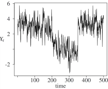
An example will be introduced. Considering an ARFIMA(0,d,0) process

(1−_L)d_Xt =ε_t,

where L is the lag operator, εt are iid random variables with zero mean and the varianceσ2

and the degree of integration is determinded by the long memory parameterd. A stationary

long memory process is characterized by the value ofd in the interval between[0,0.5].

Ford=0.2, a sample size ofT =500 and two breaks from µ1=3 to µ2=0 and µ3=3 at

t1=200 andt2=350 an exemplary time series is shown in figure 1.

Figure 1: Exemplary time series with two breaks in the mean

Xt

-2 2 4 6

100 200 300 400 500 time

In figure 2 the spanned regression tree is presented. There are four leaves and each is

att1=200,t2=294 andt3=351. The different estimated mean levels are noted below the

encircled numbers.

Figure 2: Regression tree after growing

t <> 351.5

t <> 200.5

3.0897235 200 obs

1 t <> 294.5

0.383134 94 obs

2

−0.5493214 57 obs

3

3.311083 149 obs

4

The growing of the tree is literally driven by the data, so after the growing process a very well

fitted tree is build, because the only stopping rule would be a lack of improvement in the sum

of RSS. In fact the tree gets often quite large and is over fitted (see Rea et al. (2008)). That’s

why pruning techniques are needed to determine which of the nodes are redundant. There is

the possibility of manual pruning which is a quite reasonable way if a priori knowledge can

be used.

A nested hierarchy of regimes was built and can be pruned back by a pruning method. They

work from bottom to top. That means that the first node to cut would be the one which was

grown last, so which gained the weakest node impurity improvement. In our example this

Pruning methods are e.g. the cost-complexity pruning (see Breiman et al. (1993)) or an

information criteria such as the BIC. Rea (2008) showed that the cost-complexity pruning

is difficult to handle because a complexity parameter (penalty parameter) has to be chosen

and that the BIC is the best information criteria over all considered cases. The penalty term

of the BIC depends on the size of the time series T and the number of terminal nodes p.

Kokoszka and Leipus (2002) show that the Bai Perron procedure which is similar to the BIC

information criteria excludes linear sequences with long-range dependence. Regarding to that

it is not astonishing that the BIC does not handle long memory reliable, which can be shown

in section 3.

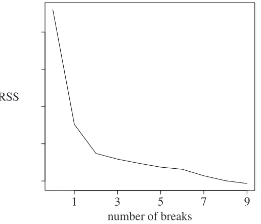
A new pruning method will be suggested to overcome this problem. The idea of the elbow

criteriais that the optimal break number is reached when the improvement of the sum of RSS

is highest. A typical shape of the sum of the squared residuals shows that there is always

a better fit by including more breaks but some splits downsize the risk function more than

others.

Figure 3:Typical shape of the sum of squared residuals depending on the break number

RSS

1 3 5 7 9

number of breaks

The largest improvement in the RSS is made where the trend has the biggest bend. To

deter-mine this bend the slope of the piecewise constant functions are considered. The last section

so an improvement of the RSS could only be minimal. Calculating the difference between

two adjacent slopes provides a measure for the improvement benefit through this splitting.

The highest benefit is defined as the optimal number of breaks.

This procedure is independent of the length of the time series and the number of terminal

nodes. It determines the optimal number of breaks where the highest improvement can be

made through splitting at that point. The advantage is that the over fitted tree which was

grown can be counterbalanced because all the small RSS improvements become irrelevant.

In comparison the BIC does depend on the height of its penalty term and though it can be

irritated by the amount of suggested break points.

The elbow criteria considers an absolute deviation between the levels of the RSS function and

can so easily respond to different levels of the RSS function through different time series and

persistences respectively. Returning to the example given before the optimal number of breaks

would be 2. In figure 3 you can see that at two breaks the improvement through splitting the

sample is highest which expresses in the biggest bend of the RSS function.

3

Monte Carlo study

An extensive Monte Carlo study will demonstrate the performance of the new pruning method

for the long-memory framework in comparison to the BIC. All simulations are computed

with the open-source programming language R (2008). The number of replications is set to

M=1000 and we consider a sample size ofT=500 in order to illustrate the good performance

in small samples. All results improve when using larger samples.

The data generating process is an ARFIMA (0,d,0) withd=0.2 andd=0.4 respectively. The

levels of the mean are chosen relatively small on purpose. Small changes e.g. fromµ1=1 to

µ2=3 are harder to determine than large level shifts. Also returning breaks (e.g. µ1=1 to

µ2=3 and back toµ3=1) are challenging, because this small peak can be easily overlooked.

The position of the mean shift when there is only one mean shift is after the 300th observation

and it will be shown that the position does not have a big influence on the results. Considering

Comparing the widespread BIC and the elbow criteria underpin the findings of Kokoszka and

Leipus (2002). The BIC is not able to handle the long-range dependencies because of the

high persistence and dependencies. The tree misspecifies local trends and cycles as additional

break points and the penalty term of the BIC is not strong enough to penalize the high

persis-tence. The BIC leads to choose the maximum number of breakpoints which is spanned by the

regression tree, so in most cases no real pruning takes place.

Table 1:Performance of BIC and elbow criteria

when there is one mean shift

elbow criteria BIC

d=0.2 mean s.d. % correct mean s.d. % correct

µ1=1;µ2=3 1.00 0.00 100.00 2.51 1.23 22.80

µ1=3;µ2=1 1.00 0.00 100.00 2.50 1.20 22.40

µ1=1;µ2=2 1.03 0.35 98.60 3.82 1.67 7.40

d=0.4

µ1=1;µ2=3 1.04 0.33 97.50 5.39 1.80 0.50

µ1=3;µ2=1 1.05 0.41 97.60 5.37 1.79 0.60

µ1=1;µ2=2 1.53 1.28 78.10 6.44 1.86 0.40

The BIC has huge problems to find only one mean shift. It overestimates the quantity by

multiple times. The higher the persistence the more mean shifts will be detected and the

lower is the quantity of a correct determination. For the elbow criteria it is not very hard

to determine this one mean shift in a stationary long memory process. The higher the level

of the mean shift and the lower the persistence the more accurate is the criteria. Hence the

mean is very close to the correct number of breaks, a very small standard deviation is obtained

and the percentage of a correct chosen number of breaks is high. The direction of the shift

(from a high level to a lower one or vice versa) influences neither the pruning criteria nor the

tree growing process. The following table 2 shows that the position of the mean shift barely

Table 2:Performance of BIC and elbow criteria

when the position of the break varies and there is one mean shift

break at observation elbow criteria BIC

d=0.2;µ1=1;µ2=3 mean s.d. % correct mean s.d. % correct

50 1.00 0.03 99.90 3.32 1.68 15.40

250 1.00 0.00 100.00 2.45 1.20 24.60

450 1.01 0.07 99.50 3.28 1.64 14.00

d=0.4;µ1=1;µ2=3

50 1.37 0.84 76.60 6.25 1.82 0.50

250 1.04 0.33 98.30 5.42 1.81 0.90

450 1.40 0.99 78.00 6.16 1.84 0.50

The results for multiple mean shifts are reported in table 3 and 4. The elbow criteria handles

more breaks much more solid than the BIC and gives good results in detecting the mean shifts.

The positions of the break points are spaced equally.

Table 3:Performance of BIC and elbow criteria

when there are two mean shifts

elbow criteria BIC

d=0.2 mean s.d. % correct mean s.d. % correct

µ1=1;µ2=4;µ3=1 2.07 0.26 95.80 2.63 0.76 52.50

µ1=1;µ2=3;µ3=1 2.15 0.39 87.20 3.36 1.13 23.90

µ1=1;µ2=2;µ3=1 2.04 0.64 67.00 4.52 1.48 7.80

d=0.4

µ1=1;µ2=4;µ3=1 2.06 0.54 70.60 4.79 1.44 3.40

µ1=1;µ2=3;µ3=1 1.92 0.75 55.10 5.85 1.58 1.20

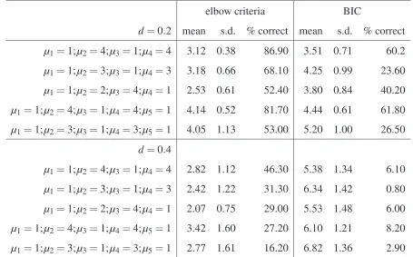
Table 4:Performance of BIC and elbow criteria for multiple mean shifts

elbow criteria BIC

d=0.2 mean s.d. % correct mean s.d. % correct

µ1=1;µ2=4;µ3=1;µ4=4 3.12 0.38 86.90 3.51 0.71 60.2

µ1=1;µ2=3;µ3=1;µ4=3 3.18 0.66 68.10 4.25 0.99 23.60

µ1=1;µ2=2;µ3=4;µ4=1 2.53 0.61 52.40 3.80 0.84 40.20

µ1=1;µ2=4;µ3=1;µ4=4;µ5=1 4.14 0.52 81.70 4.44 0.61 61.80

µ1=1;µ2=3;µ3=1;µ4=3;µ5=1 4.05 1.13 53.00 5.20 1.00 26.50

d=0.4

µ1=1;µ2=4;µ3=1;µ4=4 2.82 1.12 46.30 5.38 1.34 6.10

µ1=1;µ2=3;µ3=1;µ4=3 2.42 1.22 31.30 6.34 1.42 0.80

µ1=1;µ2=2;µ3=4;µ4=1 2.07 0.75 29.00 5.53 1.48 6.00

µ1=1;µ2=4;µ3=1;µ4=4;µ5=1 3.42 1.60 27.20 6.10 1.21 8.20

µ1=1;µ2=3;µ3=1;µ4=3;µ5=1 2.77 1.61 16.20 6.82 1.36 2.90

The chosen transitions are quite regular which is much more difficult to detect for a break

point estimator than extreme breaks. This almost cyclic behavior (fromµ1=1 toµ2=4 and

back toµ3=1 andµ4=4) simulates the most challenging break pattern with local cycles and

persistences best. Hence the good behavior in this cases are very founded results for more

obvious (easier to be detected) breaks.

Finally you can say that the BIC overestimates the number of breaks with high standard

de-viations. The percentage of correct chosen breaks is so small that even educated guessing

would be more successful. The ability of the elbow criteria on the other hand stays reasonable

even if there is more than one mean shift. When the persistence increases the criteria tends

to underestimate the number of mean shifts. The elbow criteria as a pruning technique of

the atheoretical regression trees shows very good properties even when multiple mean shifts

with small level changes occur in a long memory time series. They will be still detected and

4

Application on inflation rates

To illustrate the good performance of the atheoretical regression trees an application to CPI

inflation rates is given. The time series data starts in January of 1960 (except Australia starts

in 1971) and ends in June 2009. The following table 5 shows the results of some OECD

countries when ART with the elbow criteria is applied.

Table 5:Break points in inflation rates

of selected OECD countries

Country 1st break 2nd break

Australia Jan 91

-Canada Aug 72 Dec 91

Germany Sep 70 May 83

Japan Dec 81

-New Zealand Sep 70 Jun 90

Switzerland Oct 93

-UK Sep 73 Nov 82

US Jul 73 Nov 82

The atheoretical regression trees find one or two breaks in the inflation rates. Corvoisier and

Mojon (2005) determined three waves where breaks in inflation rates occur. In their opinion

since 1960 most OECD countries had breaks around 1970, 1982 and 1991. This can be very

well encountered by the estimated break points via ART. Hsu (2005) identifies the break points

under the assumption of two known breaks and finds for Germany the breaks at October 1969

and July 1982 and for the US at January 1973 and September 1981. Under the assumption of

one appearing break he determines for the japanese inflation rate the break point at May 1981.

Hence most of his results are very close to the specified breaks by the elbow criteria, however

Hsu has to know a priori how many breaks will occur.

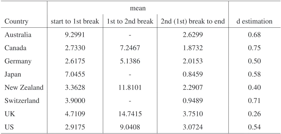
After demeaning the inflation rates using the specified break points the long memory

parame-ter can be computed by the GPH estimator. In the following table 6 the mean of each regime

Table 6:Mean of each break regime and demeaned d estimation of selected OECD countries

mean

Country start to 1st break 1st to 2nd break 2nd (1st) break to end d estimation

Australia 9.2991 - 2.6299 0.68

Canada 2.7330 7.2467 1.8732 0.75

Germany 2.6175 5.1386 2.0153 0.50

Japan 7.0455 - 0.8459 0.58

New Zealand 3.3628 11.8101 2.2907 0.40

Switzerland 3.9000 - 0.9489 0.71

UK 4.7109 14.7415 3.7510 0.26

US 2.9175 9.0408 3.0724 0.54

The detected breaks in the inflation rates have quite high level differences. When there are

two breaks in the inflation rate the mean before the first break and after the second break is

often almost the same and a large peak between the breaks can be detected. In this situation

(when the transitions are quite regular) ART showed good properties (see section 3) and hence

underpin that these break point findings are quite reliable. After demeaning the data

accor-dingly to the estimated break points long-range dependencies are still present in the data. This

implies that an approach which accounts for long memory and mean shifts is very rational.

5

Conclusion

In this paper a new pruning technique for atheoretical regression trees is invented. When the

data generating process is long memory and has shifts in the mean function it performs much

better than common pruning methods like the BIC. In a stationary long memory framework the

elbow criteria accomplishes the detection of the breaks no matter how many shifts appear and

where they are situated, even in small samples. With increasing persistence and decreasing

shift level the determination gets slightly underestimated. As the procedure is well grounded

it can also be extended for smooth transition trees (da Rosa et al. (2008)) and to trend or

References

Breiman, L., Friedman, J.H., Olshen, R.A. and Stone, C.J. (1993): Classification and

Re-gression Trees.Chapman & Hall, New York.

Brown, R.L., Durbin, J. and Evans, J.M. (1975): ”Techniques for testing the constancy of

regression relationships over time.”Journal of the Royal Statistical Society B37, 149 –

163.

Cappelli, C. and Reale, M. (2005): ”Detecting Changes in Mean Levels with Atheoretical

Regression Trees.” Research Report UCMSD2005/2, Department of Mathematics and

Statistics, University of Canterbury.

Chow, G.C. (1960): ”Tests of equality between sets of coefficients in two linear regressions.”

Econometrica28, 591 – 605.

Corvoisier, S. and Mojon, B. (2005): ”Breaks in the Mean of Inflation: How they happen

and what to do with them.” ECB Working Paper No. 451.

da Rosa, J.C., Veiga, A. and Medeiros, M.C. (2008): ”Tree-Structured Smooth Transition

Re-gression Models Based on CART Algorithm.” Journal of Computational Statistics and

Data Analysis52, 2469–2488.

Diebold, F.X., Inoue, A. (2001): ”Long memory and regime switching.” Journal of

Econo-metrics105, 131–159.

Granger, C., Hyung, N. (1999): ”Occasional Structural Breaks and Long Memory.”

Univer-sity of California, San Diego, Discussion Paper99.14.

Hsu, C.-C. (2005): ”Long memory or structural changes: An empirical examination on

in-flation rates.” Economics Letters88, 289 – 294.

Kokoszka, P. and Leipus, R. (2002): ”Detection and estimation of changes in regime” In:

Long-range Dependence: Theory and Applications by P. Doukhan, G. Oppenheim and

Ploberger, W. and Krämer, W. (1992): ”The CUSUM test with OLS residuals.”

Economet-rica60(2),271 – 285.

R Development Core Team (2008): ”R: A language and environment for statistical

comput-ing.” Available at www.r-project.org.

Rea, W.S. (2008): ”The Application of Atheoretical Regression Trees to Problems in Time

Series Analysis.”PhD Thesis.Department of Mathematics and Statistics, University of

Canterbury.

Rea, W.S., Reale, M., Cappelli, C. and Brown, J.A. (2008): ”Identification of Changes in

Mean with Regression Trees: An Application to Market Research.” Econometric

Re-views.forthcoming.

Sibbertsen, P. (2004): ”Long-memory versus structural change: An overview.” Statistical