Variable Ticket Pricing in Major League
Baseball
Daniel, Rascher and Chad, McEvoy and Mark, Nagel and
Matt, Brown
University of San Francisco, Illinois State University, University of
South Carolina, University of South Carolina
2007
Online at
https://mpra.ub.uni-muenchen.de/25803/
Running Head: Variable Ticket Pricing
Variable Ticket Pricing in Major League Baseball
Daniel A. Rascher
University of San Francisco
Chad D. McEvoy
Illinois State University
Mark S. Nagel
University of South Carolina
Matthew T. Brown
University of South Carolina
Daniel A. Rascher
Sport Management Program
University of San Francisco
Lone Mountain Pacific Wing 116
2130 Fulton St.
Variable Ticket Pricing in Major League Baseball
Abstract
Sport teams have historically been reluctant to change ticket prices during the
season. Recently, however, numerous sport organizations have implemented variable
ticket pricing in an effort to maximize revenues. In Major League Baseball, variable
pricing results in ticket price increases or decreases depending on factors such as quality
of the opponent, day of the week, month of the year, and for special events such as
opening day, Memorial Day and Independence Day (July 4). Using censored regression
and elasticity analysis, this paper demonstrates that variable pricing would have yielded
approximately $590,000 per year in additional ticket revenue for each Major League
team in 1996, ceteris paribus. Accounting for capacity constraints, this amounts to only
about a 2.8% increase above what occurs when prices are not varied. For the 1996
season, the largest revenue gain would have been the Cleveland Indians, who would have
generated an extra $1.4 million in revenue. The largest percentage revenue gain would
have been the San Francisco Giants. The Giants would have seen an estimated 6.7%
Variable Ticket Pricing in Major League Baseball
Variable ticket pricing (VTP) has recently been a much-discussed topic in the
business of sport, especially as it relates to professional baseball, professional hockey,
and college football (King, 2003; Rovell, 2002b). VTP refers to changing the price of a
ticket to a sporting event based on the expected demand for that event. For example,
Major League Baseball’s (MLB) Colorado Rockies had four different price levels for the
same seat throughout the season (Cameron, 2002). The different price levels were based
primarily on the time of the year (summer vs. spring or fall), day of the week (weekends
vs. weekdays), holidays (Memorial Day, Independence Day, etc.), the quality of the
Rockies’ opponent, or their opponents’ star players (e.g., Barry Bonds). The same seat in
the outfield pavilion section of Coors Field, the Rockies’ home stadium, ranged in price
in 2004 from a high of $21 for what the Rockies labeled as “Marquee” games to a low of
$11 for what were considered “Value” games. MLB teams who utilized variable ticket
pricing in 2004 are detailed in Table 1. Other sport organizations besides MLB
franchises utilize VTP as well. Several National Hockey League (NHL) teams utilize
VTP strategies, as do a number of intercollegiate athletics programs (Rooney, 2003;
Rovell, 2002b).
-- Insert Table 1 about here --
Some MLB teams have concluded that their 81 home games are not 81 units of
the same product, but rather, based on the aforementioned characteristics such as the day
of the week and quality of the opponent, are 81 unique products. As such, the 81 unique
products should each be priced according to their own characteristics that make them
notion. For example, in a study including more than 50 independent variables in
explaining MLB game attendance, McDonald and Rascher (2000) found variables such
as day of the week, home and visiting teams’ winning percentages, and weather among
many others to be statistically significant predictors of game attendance. Clearly, a
variety of factors make some games more appealing and others less appealing to
consumers. It seems quite logical to price tickets to these games at different price levels,
especially with teams constantly searching for revenue sources to compete with their
opponents for players (Howard & Crompton, 2004; Zimbalist, 2003).
Varying quality of games throughout a season often creates a secondary market,
as demand for the most popular games may exceed available supply. Independent ticket
agents, or scalpers, broker tickets obtained from various sources to fans unable or
unwilling to purchase tickets from a team’s ticket office or licensed ticket agency (Caple
2001; Reese, 2004). Ticket scalpers respond to market demands (often in violation of
city ordinances or state laws), but the team initially selling the ticket does not realize any
increased revenue during a scalper’s transaction (“History of Ticket Scalping,” n.d.). For
this reason, the Chicago Cubs have recently permitted ticket holders to auction their
Wrigley Field tickets on a Cubs affiliated website with a fee being paid to the Cubs for
this service (Rovell, 2002a; see also www.buycubstickets.com). It is believed that
instituting a comprehensive VTP policy would diminish the influence of scalpers and
permit greater revenue to be generated by the team for highly demanded games.
Many industries have previously embraced the variable pricing concept as a
method to increase revenue and to provide more efficient service to consumers (Bruel,
week (Monday, Fridays), times of the day (morning, late afternoon), and days of the year
(holidays), when travel demand is higher. The airlines also utilize variable pricing to
encourage passengers to book their flights early (typically a purchase at least 10-14 days
in advance generates a lower fare) or in some cases at the last minute (“Travel Tips,”
2004). Hotel pricing characteristically reflects expected demand, even though the actual
physical product does not change, as rooms for weekends or holidays are usually higher
priced than weekdays or off-season visits. In fact, sometimes variable pricing even relates
to major sporting events like the Super Bowl. Many hotels substantially raise room rates
during Super Bowl week (Baade and Matheson, n.d.). Other industries, like
transportation, utilize variable pricing, where some toll roads now charge higher toll rates
during peak times and lower rates during off-peak times (“Group Commends…,” 2001).
The arts use variable pricing as well, such as matinee movie pricing (Riley, 2002).
Sports franchises are moving forward with VTP strategies before sufficient
research has been done to empirically evaluate its specific merits to the industry. This
article provides a straightforward assessment of optimal VTP. First, a review of the
literature reveals difficulties in estimating the nature of demand functions in sports.
Specifically, optimal pricing is partially determined by price elasticities of demand, yet it
is difficult to estimate ticket price elasticities that are consistent over time. Next, a theory
of complementary demand is explained that will account for non-ticket products and
services and the effect that ticket prices have on the demand for these products and
services. Then, using individual game data from the 1996 MLB season, ticket prices and
corresponding quantities are estimated that would have maximized ticket revenue. These
variable ticket pricing policy. The final section contains a discussion of the implications
of the results. In summary, this article shows that there are financial benefits from
implementing VTP, details how much can be gained from a general VTP policy, and
provides strategies for implementing VTP.
Review of Literature
Price Elasticity of Demand in Sports
While the literature specifically investigating VTP in sport is limited, the
literature on estimating demand functions and the corresponding elasticities for sporting
events is extensive. Typically, these studies estimate the price elasticity of demand to see
whether sports teams are setting price to maximize revenue (or profit if it can be shown
that variable costs are relatively negligible). In practice, one could adjust season ticket
prices and institute a VTP policy that increases revenue based on the results of elasticity
studies. One problem is that the results are not consistent across studies. One explanation
for this is that it is reasonable for prices to be set in the elastic, inelastic, or unit elastic
portion of demand under various circumstances. For instance, profit maximization
results in prices that are in the elastic portion of demand if marginal costs are above zero.
If marginal costs are not above zero, then optimal prices are such that profit
maximization equals revenue maximization – and that occurs at unit elasticity. However,
if other revenue streams are accounted for, such as concessions or parking, then optimal
pricing can be in the inelastic portion of demand. Thus, each of these three demand
elasticity pricing strategies is justifiable. It is generally assumed in sports ticket pricing
demand not optimal in terms of pricing. Any price from unit elasticity down into the
inelastic portion of demand is a likely finding as shown in the literature.
Noll’s (1974) point estimates for elasticity for baseball were -0.49 for the 1970
and 1971 seasons. For the 1984 MLB season, Scully (1989) estimated point elasticities
of -0.63 and -0.76. Boyd and Boyd (1996) used Scully’s 1984 data, but added a measure
of competition (recreational index for each city) and used a recursive feedback loop that
incorporated the effects of home field advantage. Namely, not only do more wins
increase attendance, but enhanced attendance improves winning as a greater home field
advantage is created. In this study, point elasticities ranged from -0.58 to -1.20. Hence,
Boyd and Boyd discovered elasticities that were in the expected range, near or above unit
elasticity. It is important to note that economists have a habit of referring to price
elasticities as being positive even though they are actually negative. A price elasticity of
–1.5 is in the expected range for a profit maximizing decision maker. In fact, any price
elasticity that is –1.0 or lower (meaning –1.5 or –2.0) is consistent with profit
maximization. However, a price elasticity of –2.0 will often be called a higher elasticity
than –0.8, referring to the absolute value of elasticity and ignoring the sign (which is
always negative).
Scully, Noll, and Boyd and Boyd’s estimates all had large enough confidence
intervals on the ticket price coefficient to not exclude unit elasticity as a possibility. In
other words, none of those studies could reject the hypothesis that teams set ticket prices
to maximize revenue. However, a study by Whitney (1988), that utilized more
observations than those discussed above, did yield an estimate of price elasticity that fell
in the inelastic part of demand using annual team-level data covering a twenty-year
period. The implications of inelastic pricing will be explained in the Theoretical
Foundations section.
Fort (2004) recently summarized the literature on spectator sports demand
analysis and the difficulty in measuring price elasticities. He noted that simply analyzing
one revenue stream makes it appear that pricing is not profit maximizing, and that a more
complete accounting of all revenue streams (e.g., tickets, concessions, and local
television) is consistent with profit maximization pricing. Given this discussion of price
elasticities and profit maximization, this study incorporates models attempting to include
the relationship between ticket and concession prices.
Ticket Pricing Issues
It has been difficult for researchers to show profit-maximizing ticket pricing by
sports teams. There are a number of reasons for this besides the inclusion of other
revenue streams. First, most pricing data that is used is a simple average of prices that
are available for various seats for each team each season. Currently, Team Marketing
Report (TMR) collects pricing data that some researchers have used (e.g., Rishe &
Mondello, 2004, and Rascher, 1999). While it is likely an improvement over previously
collected pricing data, it has lacked consistency across teams and over time. Numerous
discussions by the authors and TMR have revealed that TMR is able to separate out the
luxury suite ticket prices. TMR has also separated out club seating prices for some
teams, but not all teams. Further, this varies across seasons. TMR relies on the teams to
self-report. Because of the prominence of the TMR Fan Cost IndexTM, some teams
the number of seats available at each price level does not typically weight these prices.
Additionally, the number of seats sold is generally known in aggregate, not separated by
seat price. Second, Demmert (1973) noted that there is a correlation between population
and ticket price across many seasons (likely based on the connection to income where
higher populated areas earn higher incomes, hence increasing demand and therefore
prices). This multicollinearity can cloud the interpretation of coefficients on price.
Third, as Salant (1992) pointed out, the long-run price of tickets may be optimal
(adjusting for risk), but in the short-run a team may be over- or under-pricing in order to
maintain consistency. This is a form of insurance where the team bears the risk. Fourth,
similar to Fort’s (2004) findings, ticket prices may be kept relatively low in order to
increase the number of attendees to an event who are likely to spend more money on
parking, concessions, and merchandise, and who will drive up sponsorship revenue for
the team, thus maximizing overall revenues rather than simply focusing on ticket
revenues.
DeSerpa (1994) discussed the rationality of apparently low season ticket prices.
Even though many games sell out in the NBA and NFL (focal sports in his study), it is
rational for the seller to price below the myopic short-run demand price in order to give a
fan a reason to purchase season tickets. In fact, DeSerpa discussed the possibility, but
unlikeliness, of charging different prices for each event based on its demand. He
surmised that it was administratively expensive and subject to potential negative fan
reaction.
DeSerpa (1994) also noted that it is optimal to under-price season tickets if fans
contests. The season ticket must be priced low enough for holders to be able to, at the
least, recoup their initial investment after assuming the transaction costs of resale (e.g.,
time, effort, search costs, and actual costs such as postage and advertising). Lower priced
season tickets also potentially created a home field advantage for teams. Each argument
or concern DeSerpa proffered can be addressed in a variable ticket pricing system.
Marburger (1997) developed a model showing that pricing on the inelastic portion
of demand can be explained by accounting for non-ticket purchases, such as concessions.
Marburger noted that baseball teams set price on the inelastic portion of demand, but he
did not investigate whether it was based on concessions decisions, just that it occurs.
Under multiple methods of measuring ticket price, Coates and Harrison (forthcoming)
found that ticket demand is also quite price inelastic.
Variable Pricing Literature
Specific to variable pricing, Heilman and Wendling (1976) analyzed ticket price
discounting by the Milwaukee Bucks of the National Basketball Association (NBA). The
Bucks discounted prices from $5 to $2 and from $3.50 to $2 for 15 games of the 1974-75
season. The fifteen 1973-74 games that corresponded to the 1974-75 discounted games
averaged 9,307 fans and had only three sellouts. The discounted 1974-75 games averaged
10,396 fans and had nine sellouts. Certainly, several factors (winter weather, player
injuries, or even reversion to the mean) beyond the discounted price could have
contributed to the attendance increases. However, other teams did not duplicate the
Bucks’ attempt to discount tickets. Though the increase in attendance may appear
minimal and be due to other factors besides discounting, when ancillary revenue sources
investigation into VTP was warranted. However, the Bucks remained one of the few
teams in American professional sport to implement a form of variable ticket pricing until
1999 (King, 2002a; Rovell, 2002a).
While some research has been conducted regarding VTP, this limited body of
knowledge is not yet sufficient to provide evidence concerning the merits of using VTP
to set single-game ticket prices for sporting events. Despite this lack of information, some
teams have implemented variable pricing, while others have remained skeptical (King,
2002a). This study investigates the financial gains of VTP and provides some direction
regarding how it should be implemented in Major League Baseball.
Theoretical Foundations
The demand for baseball games changes from game to game, partially because the
quality and the perception of the quality of the home and visiting teams vary as well as
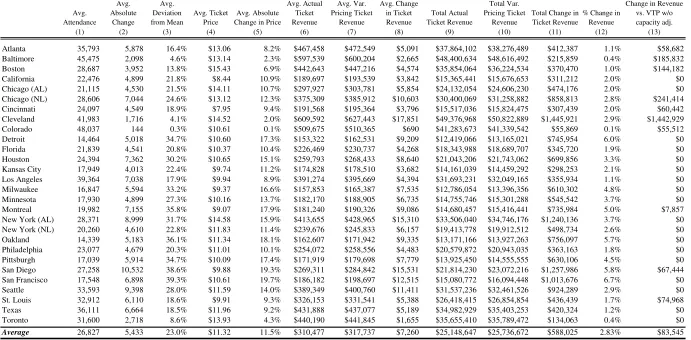
non-performance factors such as day of the week or month. For a given price, Table 2
(columns 2 and 3) shows that there is a large variance in attendance across games. The
average deviation from the mean is nearly 23%. For 11 of the Atlanta Braves’ 81 home
games, the deviation from the mean is over 30%, and the Braves are not even in the top
half of teams with high attendance variation.
Insert Table 2 about here.
In general, many organizations are trying to minimize the effect of team
performance, one of the key factors in the changing demand from game to game, on
demand (Brockington, 2003; George, 2003). As shown in the literature, team
owner. For example, Bruggink and Eaton (1996) and Rascher (1999) analyzed
game-by-game attendance and the importance of team performance. Using annual data, Alexander
(2001) showed that the variable with the highest statistical significance is the number of
games behind the leader, a measure of team performance. Teams are building new
stadiums, improving concessions and restaurants, and creating areas where kids and
adults can enjoy themselves, but not necessarily watch the game itself (George, 2003).
These improvements not only increase demand, but also lessen the importance that team
performance uncertainty has on expected revenues.
Concurrently, teams are beginning to use variable pricing to attempt to manage
shifting demand from game to game given that they are unable to completely remove the
variation. The theory upon which this analysis is based is simply short-run revenue
maximization with two goods that are complementary. Tickets and concessions are
complementary goods. The demand for tickets is higher if concessions prices are lower
because the overall cost of enjoying the game would be higher (Marburger, 1997; Fort,
2004). Similarly, the demand for concessions is higher if ticket prices are lower. The
model consists of demand for tickets and a separate aggregate demand for non-ticket
products and services (hereafter referred to as concessions) that is affected by ticket price.
This is where the complementarity between the two demand functions occurs. The three
models below describe increasing degrees of complexity for the relationship between
ticket demand and concessions demand. As shown below, VTP policies should account
for the extent to which complementarity exists between ticket demand and non-ticket
demand.
1 1 1
1 P
Q =α −β (1.1)
be the demand for tickets, where Q1 is quantity demanded, P1 is ticket price, and α1 and
1
β are scalars describing the shape of the demand curve. In this model, the demand for
concessions, , will be unaffected by ticket prices. The optimal revenue maximizing
ticket price is 2 Q 1 1 * 1 2β α =
P . (1.2)
The price elasticity of demand (ηPQ) at and , where
* 1
P Q1* 12 1
* 1 = α
Q , is equal to negative
one, a common result from microeconomic theory. Thus, in the model, price is chosen
whereηPQ =−1. This model is applicable for teams that do not share in concessions
revenues or simply receive a fixed annual payment for concessions rights from a vendor,
perhaps having sold them up front to build a new stadium. In general, much of the costs
associated with operating a baseball team are fixed costs. The marginal costs of selling
an extra ticket are low; hence revenue maximization will be assumed in place of profit
maximization. Relaxing this assumption adds a marginal cost term to the analysis, but
does not change the fundamental findings. The marginal costs of MLB teams are
unknown, and therefore the empirical analysis does not incorporate it.
Model 2 is applicable for teams that receive all or a share of concessions revenue.
Let
1 1 1
1 P
Q =α −β (2.1)
be ticket demand as in Model 1. Further, letQ2 =Q1, meaning that each person who
exogenously determined by the concessionaire and will be noted byP2. Note that
concessions do have a non-negligible marginal cost that affects total profitability. A
more complete model would include marginal cost in the final optimal ticket price setting
equation. However, this would add unnecessary complexity, and more importantly, make
it more cumbersome to compare to Model 1 to see how price is affected. The resulting
optimal revenue maximizing ticket price is
2 2 2 1 1 * 1 P
P = −
β α
. (2.2)
As seen in Equation 2.2, the revenue maximizing, or optimal, ticket price is lower
when accounting for the price of concessions (and any other non-ticket products/services
such as merchandise and parking) than it would be if it were set in a vacuum where only
ticket revenue is accounted for, as in Equation 1.2. This is consistent with findings in the
review of literature above. Specifically, 1
) ( ) ( 2 1 1 2 1 < ⎥⎦ ⎤ ⎢⎣ ⎡ + − = P P
PQ α β
α
η , meaning that the
elasticity for Model 2 is smaller in absolute value terms than for Model 1. The optimal
ticket price is set in the inelastic portion of demand. Predictably, for low concessions
prices, the impact of concessions revenue on ticket price decision making is minimized.
In fact, P2 →0,ηPQ →−1, which is the optimal price elasticity when not accounting for
concessions revenues (Model 1).
Model 3 generalizes Models 1 and 2 by adding cross-price effects to ticket
demand and concessions demand exhibiting the notion that the total price of attending a
game is what matters to customers, not just ticket price. Therefore, let
2 1 1 1 1
1 P P
Q =α −β −γ (3.1)
demand. The demand for concessions will be shown by 1 2 2 2 2
2 P P
Q =α −β −γ . (3.2)
As noted in the equation, ticket price, , affects the demand for concessions in a negative
way. If ticket prices are raised, the demand for concessions declines based on 1
P
2
γ , the
marginal propensity to purchase concessions based on ticket price changes. The optimal
revenue maximizing ticket price is
1 2 2 1 1 1 * 1 2 ) ( 2 β γ γ β α P
P = − + , (3.3)
with exogenous. Even though the concessionaire often sets concessions prices,
removing this assumption does not change the direction of the impact, only the
magnitude. Equation 3.3 shows that the ticket prices ought to be lower if fans care about
concessions prices. Specifically, higher 2
P
1
γ or γ2 leads to lower optimal ticket prices.
The more sensitive customers are to the price of complementary goods and services, the
lower ticket prices should be to maximize profits. Thus, it is important to account for
cross-price effects when setting prices. Overall, the price elasticity for Model 3 may be
higher or lower than for Model 2, depending on the relative magnitudes of β1, γ1, and
2
γ . However, like Model 2, the absolute value of the price elasticity for Model 3 is
lower than for Model 1. In the analysis that follows, variable pricing outcomes will be
determined under two scenarios, one without the cross effects (Model 1) and one with the
cross effects (Model 3). Again, Model 1 pertains to teams that either do not receive any
concessions revenue or receive a fixed payment in exchange for concessions rights.
Model 3 applies to teams that receive a share of concessions revenues.
or something else, only that a team’s objectives are consistent throughout the season. For
example, if a team is focused primarily on profits, it will set ticket and concessions prices
in order to maximize the sum of both revenues. Similarly, if a team is attempting to
maximize wins, it will still want to price as a profit-maximizer because its relevant costs
are not variable. Such a team would likely spend more on players, in order to improve
winning, than a profit-maximizing team. However, it will still want to set prices in order
to maximize revenues from tickets and concessions anyway, just as a profit-maximizing
team would. An exception to this argument is if a win-maximizing owner chose to price
below profit-maximizing levels in order to raise attendance (even though it is lowering
revenues) to increase the impact of home-field advantage, which would increase the
likelihood of winning more games and, therefore, satisfy his/her objectives.
The models also do not need to assume linear demand functions. Linear demand
is chosen for simplicity. As described in the next section, non-linear demand changes the
magnitudes of the findings. Using linear demand generates more conservative findings –
the gains to be had from variable pricing are lower under linear demand.
The empirical analysis operationalizes this by noting that whatever objective
function an owner has (winning or profits or a combination of the two), it is assumed that
prices are set to maximize those objectives. For a particular game it may be that prices
are too low or too high given demand, but since one price is charged for the entire season,
it is objective-maximizing on average.
One hypothesis stemming from these models is that adoption of variable ticket
pricing would improve revenues for MLB teams. Another hypothesis is for those teams
had only raised their prices for VTP games by $2 for 2002. In contrast, the Rockies have
had prices for particular seats that varied by as much as $6 (Rovell, 2002a). This analysis will provide a benchmark for how much teams should be adjusting their prices.
It is important to note that there are public relations issues that play a role in VTP.
For example, the Nashville Predators have been thinking about incorporating VTP but
fear a negative fan backlash at a time they are trying to build a loyal fan base (Cameron,
2002). A team therefore may opt to raise its prices only nominally to see if there is a
backlash where fans react with an emotional response that actually shifts demand (not
slides along demand as price changes are expected to do). This analysis ignores any
public relations issues.
Methods
The first analysis tested Model 1 where only ticket pricing is accounted for, not
concessions quantity and price. The methodology involved analyzing how demand for
each game deviated from the average demand for each team. For example, as shown in
Figure 1, point ‘A’ is on the average demand curve for the Atlanta Braves. It represents
the actual average ticket price ($13.06) and average attendance (35,793). The slope of
the demand curve is based on the assumption that the price elasticity equals -1.0 (This
assumption can be relaxed without loss of generality. For instance, it can be assumed
that the team prices on the inelastic portion of demand at, say, -0.75). Therefore, slope
can be determined from price, quantity, and elasticity.
Insert Figure 1 about here.
home opener. This is the demand for that game given the price. Demand is known
because looking at actual attendance reveals it. As described in the Theoretical
Foundations section, ticket prices, on average, were optimal for the Braves. It was
assumed that each team was doing its best at determining ticket prices and was setting
them to account for the average expected demand for the entire season. Therefore, the
price elasticity was set at -1.0 at point ‘A’. At point ‘B’ the elasticity changed to –0.73,
thus it is a sub-optimal price. Raising price to $15.46 (point ‘C’) changed the elasticity
back to –1.0 and lowered attendance to 42,371. Revenue was then calculated for this new
price and quantity and compared to the actual revenue from that game (measured by
multiplying the actual average price charged for that game with the actual quantity of
spectators for that game). These measurements were taken for each game of the season
for each team in order to be able to see how adjusted ticket prices affect revenue. See the
Appendix for a brief description of the calculations.
The example above used linear demand. If a slightly curved demand function is
used, the gains from variable pricing would be higher because the loss in number of
attendees is compensated by higher pricing due to the curvature of the demand function.
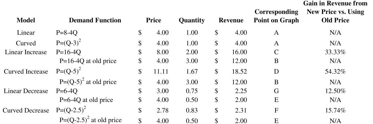
As shown in Figure 2, the simplified demand function “Curved Increase” had an optimal
price point at “D”, while the linear demand function’s optimal price point was “C”.
Table 3 provides the details of each of these demand functions. Each demand function
was shifted the same amount (as shown by point “B”). Figure 3 shows the associated
revenue at each point. The curved demand resulted in higher revenue ($18.52) from
variable pricing (point “D”) than for the linear demand ($16.00 at point “C”). Thus, an
instead of curved demand. This is also true for a low demand game. Point “G” is the
optimal price for the linear demand function and point “F” maximizes revenue for the
curved demand. As shown in Table 3, the curved demand function resulted in higher
revenues from variable ticket pricing. Intuitively, this was not surprising. For a given
price, a curved demand function will result in more attendees (higher quantity) than a
linear demand function. A constant elasticity of demand function (CED) has more
curvature than the ones shown in Figure 2. Revenue is constant regardless of price for
CED. Prices can be set at any level and yield the same revenue. CED is an unrealistic
demand function for baseball. An even more extreme demand function, a super-curved
demand in which the degree of curvature is greater than that for CED, is such that the
revenue function looks U-shaped, not hill-shaped as in Figure 3. In that case, revenue
maximizing prices are either very low or very high, and unlikely to be consistent with
reality in baseball. An example of this type of demand function isP=1ln(Q). The use of
linear demand in the subsequent analysis is conservative in that the gains from variable
pricing are a lower bound of what would be the case if demand functions for baseball are
curved. This reason, along with simplicity and a lack of research about the shape of
baseball demand functions, was justification for using linear demand in the following
analysis. Parallel shifts of the demand function were also assumed because of simplicity
and a lack of relevant research showing other types of shifts. Unfortunately, attendance
by seat location and specific price is not publicly available. If it were, one could examine
how much demand changes per price point to get a sense of the nature of the shift in
demand.
The subsequent analysis accounted for the possibility that the capacity of a
stadium prevented the true demand from being revealed. In other words, sellouts
typically imply that there was excess demand beyond the capacity of the stadium. The
standard result would be to raise prices until the entire stadium is full and there are no
persons outside who are interested in attending the game at the new raised ticket price. In
order to determine how much to raise prices, the amount of excess demand needed to be
estimated. This was done utilizing a censored regression, which can forecast the true
demand as if there were not a capacity constraint. It used information from uncensored
observations (those without a capacity constraint as shown by not having sold out) to
estimate what would have happened without the constraint.
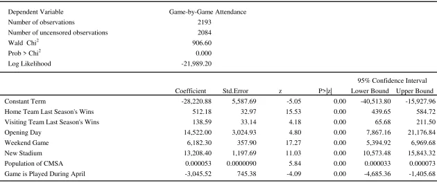
The censored regression used attendance as the dependent variable and various
demand factors listed in the second data set described below as the independent variables.
The result was an empirical model that can be used to forecast what attendance would
have been for the capacity constrained games. The methodology was the same as the first
analysis, but used the new forecasted attendance when estimating optimal prices and
resulting revenue.
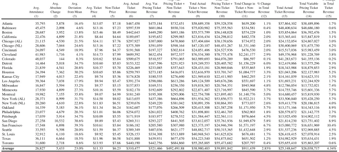
The final analysis included the focus of Model 3, that the prices of
complementary goods (tickets and concessions) affect the demand, and hence optimal
price, for each other. This analysis created a single demand for the joint product of
tickets and concessions, with concessions price exogenously determined. According to
Financial World, these non-ticket revenues made up 35% of ticket plus non-ticket
spent at a stadium by a patron, thirty-five cents were spent on concessions, merchandise
and parking. Therefore, the non-ticket price for each team was set at 54% (54% =
35%/[1-35%]) of the ticket price as team-specific data on non-ticket revenue was
unavailable. Given this new joint demand function, optimal prices were set for each
game as in the two previous analyses. The censored regression forecasts of attendance
were used in this analysis. This analysis accounted for the combined product of tickets
and concessions, so as a group the demand elasticity was -1. Given that the concessions
price was fixed and positive, the new optimal ticket price would be on the inelastic
portion of demand. This was consistent with the findings in the literature.
These three analyses determined the optimal variable ticket price for nearly every
game for the 1996 MLB season. The 1996 season was used because during that year no
MLB team utilized variable ticket pricing. It should be noted that 1996 was the first full
season after the strike of 1994-95. It is possible that the findings here are not typical of a
season in Major League Baseball. However, an important factor in this analysis is the
shift in demand from game to game. Compared with 2003, attendance for the 1996
season has a standard deviation that is only 5% greater than attendance for 2003. The use
of more recent data, which would include teams using VTP, raised validity concerns with
the attempt to predict additional revenue generated through the use of VTP. The use of
the 1996 data allow the analysis to be consistent across all teams. The analysis showed
what ticket price should have been charged with the corresponding results had every team
participated in optimal VTP. In order to achieve this, data for 2,193 of the 2,268
scheduled regular season games was used. The few games not used in the analysis either
The data was broken into two sets. One set was used to forecast optimal VTP. It
included actual attendance, average ticket price, stadium capacity, and average
concessions expenditures. Attendance data came from www.sportsline.com, ticket price
data from Team Marketing Report, stadium capacity data from www.ballparks.com, and
concessions information from Financial World’s financial report on baseball for the 1996
season (Badenhausen & Nikolov, 1997). Table 2 (columns 1 & 4) shows average
attendance and average ticket price for each team for the 1996 season.
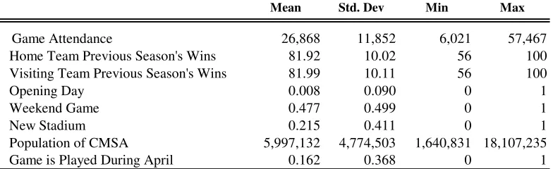
The second set of data was used to make an adjustment to demand for games that
are censored by capacity constraints, namely games that are sold out or nearly sold out.
This adjusted demand was then used in the VTP analysis. This data set contained actual
attendance, the number of wins by the home team and visiting team in the previous
season, the population of the local CMSA, indicator variables for opening day, a new
stadium, a weekend game, and a game in April. All data for this data set came from
www.sportsline.com except population, which was obtained from the U.S. Census
Bureau. Table 4 contains summary statistics of the data.
Insert Table 4 about here
Results
Based on the estimates from the test of Model 1, had the Atlanta Braves, for
example, raised ticket prices for the opening game, actual attendance would have been
42,371 with actual ticket revenues increasing by $15,817 or 2.5% for that game. An
elasticity of –1.0 implies revenue maximization. Yet, the analysis could have begun with
(see Figure 1). Therefore, this does not require revenue maximization or profit
maximization, only consistency in terms of the objectives of the franchise throughout the
season.
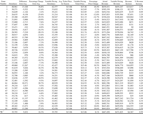
Continuing with the Braves example, Table 5 shows the results for every odd
home game. The findings show that there are fewer games that have excess demand
(although they have a higher average excess demand) than there are games that have
lower demand than average (Figure 4). In fact, 30 out of 81 Braves home games had
demand exceed the average, and the average optimal price increase is estimated to be
11.0% while the average decreased price is estimated to be -6.5%. Also, as expected, the
high demand games generally are for an entire series. Thus, one VTP strategy for the
Braves would be to variable price for some high demand series and simply lower prices
on the other games in general (as a public relations move and to increase overall
revenues).
Insert Table 5 and Figure 4 about here
The bottom row of Table 5 shows the average results for the entire Braves season.
The average per game revenue increase for the season is $4,367 or 0.9%. The results for
each team are shown in Table 2. Columns 8 and 12 show the result from Table 5 for the
Braves. Over the course of the full season, the Braves could have increased their ticket
revenues by $353,706 or 0.9%.
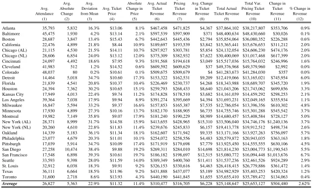
Variable pricing would have yielded an average of approximately $504,000 per
year in additional revenue for each Major League team, ceteris paribus, or over $14
what occurs when prices are not varied, as shown in Table 2. The amount of variation in
ticket prices is just over 11%, on average. That such a large price swing only yields a
revenue swing four times smaller is simply based on the large change in attendance that
occurs when prices are varied. This occurs with all downward sloping demand curves,
and is not unique to baseball. For the 1996 season, the largest revenue gain would have
been for the New York Yankees, which would have generated an extra $1.24 million in
ticket revenue, or a 3.7% increase. The largest percentage revenue gain would have been
for the San Francisco Giants. The Giants would have seen an estimated 6.7% increase in
revenue, or $1.01 million, had they used optimal VTP. The smallest amount of impact
would have been for the Colorado Rockies, which averaged only plus or minus eighty
patrons in absolute deviation from the mean attendance per game throughout the 1996
season. In fact, teams with the lowest average attendance benefit the most from variable
pricing. This is not surprising since those teams tend to have the highest variation in
attendance allowing them to gain from dynamic pricing.
The reason that the Rockies would apparently gain the least from VTP is that it
had many sellouts in 1996. As described in the Methodology section, a censored
regression is carried out in order to forecast the true demand above the capacity
constraint. While there are many more factors that affect game-by-game attendance than
those used here, this analysis used only those factors known prior to the time ticket price
setting occured. Thus, only factors known prior to the beginning of the season are used
to be consistent with what would be known by team management when setting prices.
The Wald Chi-squared test of significance showed that the model was significant at the
series between two teams may not be independent. It is expected that across different
groups of games (a three game series for example) there exists independence of the
errors, but not necessarily within each group. This type of clustered correlation leads to
understating the standard errors. A robust estimator of the variance is used to correct the
standard errors. There is no evidence of multicollinearity among the independent
variables. As expected, there is evidence of omitted variables missing from the
regression. As explained above, performance-specific factors that are only known to
price setters once the season has begun, such as the home pitcher’s earned run average at
that point during the season, were omitted. The variance-inflation factor (VIF) averaged
1.19 across the group of variables tested for multicollinearity, with the largest VIF at
1.58. The Ramsey RESET test shows evidence of omitted variables with an F-statistic of
29.67.
Table 6 shows the results of the censored regression. The signs of the coefficients
are as expected. Out of 2,193 games, only 109 were sold out. A sellout for these
purposes is defined as any game where actual attendance is 99.0% or higher of stadium
capacity. The estimate of attendance for these 109 games is based on the predicted
values from the censored regression.
Insert Table 6 about here
As shown in Table 7, ten teams had adjustments to their attendance based on the
censored regression. The results are similar to that for Table 2 except column 13 shows
the gain for those ten teams, versus Table 2, if they account for the capacity constraint
stadium capacity raises the increased revenue from VTP policies from $14.1 million to
$16.5 million for the league as a whole.
Insert Table 7 about here.
The final analysis addressed Model 3 from the Theoretical Foundations section
by accounting for non-ticket revenues such as concessions, merchandise, and parking.
Table 8 shows the results of allowing the team to vary ticket prices while accounting for
non-ticket prices in order to maximize its objectives.
Insert Table 8 about here.
Columns 9, 10, and 11 in Table 8 illustrate that the average team would have
gained $911,000 in ticket and non-ticket revenue by adopting a variable ticket pricing
policy while accounting for non-ticket prices. The league overall would have gained
$25.5 million. The Cleveland Indians would have earned the most, over $2.2 million,
from such a policy.
Discussion
This analysis has shown that Major League Baseball could have increased ticket
revenues by approximately 2.8%, or $16.5 million, and total stadium revenues by about
$25.5 million for the 1996 season if teams utilized VTP. Total revenues in MLB are
estimated to have grown from $1.78 billion in 1996 to approximately $4.3 billion in
2003, or 250%. Similar changes in the effect of VTP strategies as discovered in this
study would yield nearly $40 million in ticket revenue and over $60 million in ticket plus
to consider and implement VTP strategies, especially since teams and the league are
constantly searching for ways to increase revenues.
The San Francisco Giants would have seen an estimated 6.7% increase in ticket
revenue, or $1.01 million, had they used optimal VTP in 1996. Interestingly, the Giants
had considered utilizing variable ticket pricing since the 1996 season because they had
noticed a huge variation in attendance patterns at Candlestick Park, the team’s then-home
facility (King, 2002a). In addition to weather issues (pleasant for day games, frigid for
night contests) in their facility, the Giants of the mid-1990s occasionally fielded teams of
lower quality. The results of this study would strongly suggest that teams in similar
facility or on-the-field talent situations maximize their revenues through VTP.
The results of this study support the utilization of VTP both to increase as well as
decrease prices from average seasonal levels. The data showed fewer games with excess
demand than those with diminished demand. However, the selected games with excess
demand deviated from the mean at a greater rate than those with decreased demand.
Currently, most MLB teams have focused their VTP strategies on the revenue potential of
increased prices from highly demanded games (King, 2002a). However, it appears that
some teams have begun to realize the potential benefit of attracting fans to less desirable
contests by lowering prices (King, 2002b). The New York Yankees sold $5 tickets in
certain sections of Yankee Stadium on Mondays, Tuesdays, and Thursdays in 2003
(King, 2003).
Lowering ticket prices for less desirable games would potentially create more
positive relationships between teams and local municipalities. Major League Baseball
facilities that are financially inaccessible to many taxpayers (Pappas, 2002; O’Keefe,
2004). Given the number of games in a typical season that have demand below the yearly
average (Figure 4), lowering prices creates an opportunity for teams to potentially attract
new or disenfranchised fans and presents local governments with a more favorable
reaction to their public policy decisions supporting the local franchise. Marketing less
desirable games with lower ticket prices as “value” games, as the Chicago Cubs,
Colorado Rockies, New York Mets, Tampa Bay Devil Rays, and Toronto Blue Jays did
in 2004, allows teams to reach market segments perhaps otherwise unreachable due to
pricing/income issues, in addition to the aforementioned public relations benefits.
Currently, teams might not want to implement multiple price points for each game
as shown in Figure 4. As discussed in Levy, Dutta, Bergen and Venable (1997), menu
costs affect the frequency and desire to change prices to reflect changes in demand or
supply. Menu costs are costs associated with physically changing prices on products,
having to look up prices to tell a customer the price for a particular game, or more
generally any costs associated with having more than one price for a product or service.
Additionally, asymmetric information, search costs, and simple confusion for customers
regarding the price for different games may cause franchises to have fewer prices for a
particular seat throughout the season than variable pricing predicts. For this reason, many
teams have only utilized a minimal number of ticket-pricing tiers, usually two-to-four, in
their variable ticket pricing system (Rovell, 2002a)
Confusion and the additional costs associated with changing ticket prices may
already be in the process of being eliminated. Kevin Fenton, Colorado Rockies senior
points for games is overcome, patrons realize that tickets can be priced like other
industries (Rovell, 2002a). In the near future, the negative fan reaction to changing ticket
price will likely be alleviated if not eliminated (Adams, 2003). Ticket offices are also
now better equipped to handle menu costs issues. Although ticket offices were not
prepared to handle extensive variable ticket pricing in the 1990s, recent technological
advances have allowed most American professional sport teams to implement new ticket
policies such as bar coded and print-at-home tickets and to prepare for extensive variable
ticket pricing in the future (Zoltak, 2002).
An initial VTP recommendation is that for every 10% increase in attendance (or
specifically, expected attendance) above the average, teams should raise ticket prices by
5% and receive a gain of 1.2% in ticket revenue. The practical use of variable pricing,
however, would entail creating at most five different prices for each seat in a stadium
throughout the season, not a different price for each game. High demand games or series
should be priced accordingly, but teams should not forget the potential benefits of
lowering price for less desired games. The present findings reinforce previous research
identifying factors such as day of the week or rivalry game as affecting demand for MLB
tickets.
Using the Atlanta Braves again as an example, the average attendance was
35,793. Based upon the variable pricing ticket prices from Table 5, the recommended
pricing schedule for 1996 would have been $12.00, $13.06, and $15.50. A descriptive
analysis of Braves attendance revealed three tiers of games that corresponded with the
three price points: games with attendance below 28,831 (greater than -1 SD from the
mean), and games with an attendance over 42,756 (greater than 1 SD from the mean). A
factor analysis of games falling within each tier was then performed to finalize the
recommended pricing schedule.
For the Braves, a Tier One game (average price of $12.00) would have included
games from the second game of the season to May 14, played Sunday to Thursday.
Fifteen games would have therefore been classified as Tier One. A Tier Three game
(average price of $15.50) would have included all games played on Saturday, opening
day, the July 4 game, the final home stand of the season, and games played after May 14
against the Los Angeles Dodgers, a former division rival. Twenty-two games would
have fallen into this tier. The remaining 44 games would have been classified Tier Two
with an average ticket price of $13.06, which was the average ticket price for the 1996
season.
The hypothesis that the few teams that are administering variable ticket pricing
are doing so properly is consistent with the findings. In fact, the present analysis shows
that optimal variable ticket pricing is managed by small changes in ticket prices. The
Giants expected to gain an additional $1 million from variable ticket pricing in 2002
(Isidore, 2002; Rovell, 2002a). The Giants VTP strategy in 2002 affected only 39 of their
81 home games (all weekend dates). The present analysis shows a gain of about $1
million for the 1996 season if optimal pricing were used by the Giants.
In 2002, the Atlanta Braves instituted a VTP strategy for 21 home games –
Fridays from May through August and Saturdays throughout the whole season. During
these games ticket prices were increased by $3, or about 14%. Testing the same policy
9% increase in price. Interestingly, the Braves actual policy is more aggressive than the
data show for 1996. The St. Louis Cardinals raised prices in 2002 for summer games by
$2, or 8%. The 1996 data show that an optimal VTP strategy would raise prices by about
9%.
Directions for Future Research
There are many areas of inquiry for the future. An analysis of more recent data
that include teams utilizing VTP is warranted. The practical application of VTP requires
one to be able to accurately forecast the relative attendance of future games. In other
words, in order to know which games to have higher prices for and which games to have
lower prices for, team management needs to know whether there is consistency from one
season to the next in terms of relative attendance. An interesting behavioral issue is
whether the implementation of VTP in earlier games affects the demand for subsequent
games.
One factor unaccounted for in this study is the marketing strategies utilized by
organizations in conjunction with VTP price levels. The projected revenue increases
identified in this study could potentially be increased substantially by incorporating VTP
pricing into teams’ marketing plans. Although many MLB teams assign each
game/product into VTP levels based on game/product characteristics, little research has
investigated how those games of varying characteristics are marketed to different
demographic segments of consumers.
In addition, research investigating education and public relations activities related
to variable ticket pricing should be conducted. Although fans may initially perceive
some “expensive” games to now become more affordable. Methods to assuage consumer
fears and to attract potentially new consumers should be researched. Additionally,
implementation costs of VTP programs, such as menu costs and staff training, should be
examined and accounted for in future economic examinations of VTP.
Finally, future research should investigate the practical application and public
reaction to future variable pricing systems utilizing technology to change prices by the
day, hour, or even minute. Few teams have implemented VTP at this point, believing that
widespread use of ticket pricing based completely on supply and demand would not be
met with agreement by some consumers (Cameron, 2002). In particular, research should
be conducted to identify methods to protect or enhance value to season ticket purchasers
when a minute-by-minute VTP policy is implemented.
References
Adams, R. (2003, January 6-13). Variable price ticket policy wins converts. Sports
Business Journal, ,p. 14.
Alexander, D. L. (2001). Major League Baseball: Monopoly pricing and
profit-maximizing behavior. Journal of Sports Economics, 2, 341-355.
Baade, R., & Matheson, V. (n.d.). Super Bowl or Super (Hyper)bole? The economic
impact of the Super Bowl on host communities. Unpublished document.
Badenhausen, K., & Nikolov, C. (1997, June 17). Sports values: More than a game.
Financial World, 166, 40-44.
Boyd, D. W., & Boyd, L. A. (1996). The home field advantage: Implications for the
pricing of tickets to professional team sports. Journal of Economics and Finance,
20(2), 23-32.
Brockinton, L. (2003, May 26-June 1). New NFL digs offer more revenue possibilities.
Sports Business Journal, p. 25.
Bruel, J. S. (2003, January 27). Finding hidden revenue under the seat cushions. Sports
Business Journal, p. 23.
Bruggink, T. H., & Eaton, J. W. (1996). Rebuilding attendance in Major League
Baseball: The demand for individual games. In J. Fizel, E. Gustafson, & L.
Hadley (Eds.), Baseball economics: Current research (pp. 9-31). Westport, CT:
Praeger.
Cameron, S. (2002, May 27-June 2). Bruins to set prices hourly. Sports Business Journal,
Caple, J. (2001, August 21). All hail ticket scalpers! ESPN Page 2. Retrieved April 16,
2003, from http://espn.go.com/page2/s/caple/010821.html
Coates, D., & Harrison, T. (forthcoming). Baseball strikes and demand for attendance.
Journal of Sports Economics.
Demmert, H. G. (1973). The economics of professional team sports. Lexington, MA:
Lexington Books.
DeSerpa, A. C. (1994). To err is rational: A theory of excess demand for tickets.
Managerial and Decision Economics, 15, 511-518.
Fort, R. D. (2004). Inelastic sports pricing. Managerial and Decision Economics, 25,
87-94.
George, J. (2003, May 26-June 1). Phillies go big with entertaining Ashburn Alley.
Sports Business Journal, p. 24.
Group commends port authority for variably priced tolls. (2001). Retrieved July 19,
2004, from http://www.tstc.org/press/322_PAtolls.html
Heilmann, R. L., & Wendling, W. R. (1976). A note on optimum pricing strategies for
sports events. In R. E. Machol, S. P. Ladany, & D. G. Morrison (Eds.),
Management Science in Sports (pp.91-101). New York: North-Holland
Publishing.
History of ticket scalping. (n.d.). Retrieved July 16, 2004, from
http://metg.fateback.com/metghistory.html
Howard, D. R., & Crompton, J. L. (2004) Financing sport (2nd ed.). Morgantown, WV:
Isidore, C. (2002, December 27). Fans to pay the price(s). CNN/Money. Retrieved July
23, 2004 from
http://money.cnn.com/2002/12/27/commentary/column_sportsbiz/ticket_prices/
King, B. (2002a, April 1-7). Baseball tries variable pricing. Sports Business Journal, pp.
1, 49.
King, B. (2002b, December 9). MLB varied ticket pricing a boon. Sports Business
Journal, p. 23.
King, B. (2003, December 1-7). More teams catch on to variable ticket pricing. Sports
Business Journal, p. 16.
Levy, D., Dutta, S., Bergen, M., & Venable, R. (1997). The magnitude of menu costs:
Direct evidence from large U.S. supermarket chains. Quarterly Journal of
Economics, 112, 791-825.
Marburger, D. R. (1997). Optimal ticket pricing for performance goods. Managerial and
Decision Economics, 18, 375-381.
McDonald, M., & Rascher, D.A. (2000). Does bat day make sense?: The effect of
promotions on the demand for Major League Baseball. Journal of Sport
Management, 14, 8-27.
Noll, R. G. (1974). Government and the sports business. Washington, D.C: The
Brookings Institute.
O’Keefe, B. (2004, March 29). Pro baseball franchise hit with unusual state audit.
Stateline.org. Retrieved July 24, 2004, from
http://www.stateline.org/stateline/?pa=story&sa=showStoryInfo&print=1&id=36
Pappas, D. (2002). The numbers (part three; part five). Baseball Prospectus. Retrieved
June 20, 2004, from
http://www.baseballprospectus.com/article.php?articleid=1305
Rascher, D. A. (1999). The optimal distribution of talent in Major League Baseball. In L.
Hadley, E. Gustafson, & J. Fizel (Eds.), Sports economics: Current research (pp.
27-45). Westport, CT: Praeger Press.
Reese, J. T. (2004). Ticket operations. In U. McMahon-Beattie & I. Yeoman (Eds.), Sport
and leisure operations management (pp. 167-179). London: Continuum.
Riley, D. F. (2002). Ticket pricing: Concepts, methods, practices, and guidelines for
performing arts events. Culture Work, 2(6). Retrieved July 19, 2004, from
http://aad.uoregon.edu/culturework/culturework20.html
Rishe, P., & Mondello, M. (2004). Ticket price determination in professional sports: An
empirical analysis of the NBA, NFL, NHL, and Major League Baseball. Sports
Marketing Quarterly, 13. 104-112.
Rooney, T. (2003). The pros and cons of variable ticket pricing. Paper presented at the
2003 National Sports Forum, Pittsburgh, PA.
Rovell, D. (2002a, June 21). Sports fans feel pinch in seat (prices). ESPN.com. Retrieved
July 20, 2004, from http://espn.go.com/sportsbusiness/s/2002/0621/1397693.html
Rovell, D. (2002b, December 31). Forecasting the sport business future. ESPN.com.
Retrieved July 12, 2004, from
http://espn.go.com/sportsbusiness/s/2002/1230/1484284.html
Salant, D. (1992). Price setting in professional team sports. In P. Sommers (Ed.),
Scully, G. W. (1989). The business of Major League Baseball. Chicago: University of
Chicago Press.
Travel tips. (2004). Retrieved July 20, 2004, from
http://clarkhoward.com/travel/tips/todays_tip.html
Whitney, J. D. (1988). Winning games versus winning championships: The economics of
fan interest and team performance. Economic Inquiry, 26, 703-724.
Zimbalist, A. (2003). May the best team win: Baseball economics and public policy.
Washington D.C.: Brookings Institution Press.
Appendix
In order to calculate the new price and quantity where revenue is maximized (η =−1) when the demand curve shifts, refer to Figure 1 at Point A and let
793 , 35
= A
Q , PA =$13.06, and set ηA =(PA QA)*(ΔQA ΔPA)=−1.
At Point C, let
377 , 42 2 ) 961 , 48 793 , 35 ( 2 ) ( + = + =
= A B
C Q Q
Q , 46 . 15 $ ) 793 , 35 06 . 13 $ ( * 377 , 42 * 1 ) ( * * − =− − =
= A C A A
C Q P Q
P η
The results for the new price and quantity rely on two attributes of linear demand
functions. First, the optimal quantity ( ) is simply the average of the old quantity ( ) and the new actual quantity ( ). Second, the new optimal price utilizes the elasticity formula,
C
Q QA
B Q 1 ) ( * )
( Δ Δ =−
= C C A A
C P Q Q P
η , and solves for . A key substitute is to
note that A P A A A
A P P Q
Q Δ =−
Δ )
( , because the inverse of the slope is constant for the old demand and new demand. Also, PA and QA are given, and ηA is set equal to -1. This
Table 1
2004 MLB Variable Ticket Pricing Programsa
Team Levels Levels (price for typical outfield bleacher seats)
Arizona Diamondbacks 3 Premier ($18), Weekend ($15), Weekday ($13) Atlanta Braves 2 Premium ($21), Regular ($18)
Chicago Cubs 3 Prime ($35), Regular ($26), Value ($15) Chicago White Sox 2 Weekend ($26), Weekday ($22)
Colorado Rockies 4 Marquee ($21), Classic ($19), Premium ($17), Value ($11)
New York Mets 4 Gold ($16), Silver ($14), Bronze ($12), Value ($5)
San Francisco Giants 2 Friday-Sunday ($21), Monday-Thursday ($16) Tampa Bay Devil Rays 3 Prime ($20), Regular ($17), Value ($10) Toronto Blue Jays 3 Premium ($26), Regular ($23), Value ($15)
Note. Different seating configurations of each stadium make comparing like seats difficult; however, this attempt was made to provide the reader with an idea of the range of price levels used by each team for similar seats.
a
Table 2
Summary of Effects of Variable Ticket Pricing (no capacity or non-ticket revenue adjustment)
Avg. Attendance Avg. Absolute Change Avg. Deviation from Mean Avg. Ticket Price Avg. Absolute Change in Price Avg. Actual Ticket Revenue Avg. Var. Pricing Ticket Revenue Avg. Change in Ticket Revenue Total Actual Ticket Revenue Total Var. Pricing Ticket Revenue Total Change in Ticket Revenue
% Change in Revenue
(1) (2) (3) (4) (5) (6) (7) (8) (9) (10) (11) (12)
Atlanta 35,793 5,832 16.3% $13.06 8.1% $467,458 $471,825 $4,367 $37,864,102 $38,217,807 $353,706 0.9%
Baltimore 45,475 1,930 4.2% $13.14 2.1% $597,539 $597,909 $371 $48,400,634 $48,430,660 $30,026 0.1%
Boston 28,687 3,847 13.4% $15.43 6.7% $442,643 $445,436 $2,794 $35,854,064 $36,080,352 $226,288 0.6%
California 22,476 4,899 21.8% $8.44 10.9% $189,697 $193,539 $3,842 $15,365,441 $15,676,653 $311,212 2.0%
Chicago (AL) 21,115 4,530 21.5% $14.11 10.7% $297,927 $303,781 $5,854 $24,132,054 $24,606,230 $474,176 2.0%
Chicago (NL) 28,606 6,854 24.0% $13.12 12.0% $375,309 $382,932 $7,622 $30,400,069 $31,017,468 $617,399 2.0%
Cincinnati 24,097 4,492 18.6% $7.95 9.3% $191,568 $194,618 $3,049 $15,517,036 $15,764,032 $246,996 1.6%
Cleveland 41,983 512 1.2% $14.52 0.6% $609,592 $609,629 $37 $49,376,968 $49,379,960 $2,992 0.0%
Colorado 48,037 80 0.2% $10.61 0.1% $509,675 $509,679 $4 $41,283,673 $41,284,030 $357 0.0%
Detroit 14,464 5,018 34.7% $10.60 17.3% $153,322 $162,531 $9,209 $12,419,066 $13,165,021 $745,954 6.0%
Florida 21,839 4,541 20.8% $10.37 10.4% $226,469 $230,737 $4,268 $18,343,988 $18,689,707 $345,720 1.9%
Houston 24,394 7,362 30.2% $10.65 15.1% $259,793 $268,433 $8,640 $21,043,206 $21,743,062 $699,856 3.3%
Kansas City 17,949 4,013 22.4% $9.74 11.2% $174,828 $178,510 $3,682 $14,161,039 $14,459,292 $298,253 2.1%
Los Angeles 39,364 7,038 17.9% $9.94 8.9% $391,274 $395,669 $4,394 $31,693,231 $32,049,165 $355,934 1.1%
Milwaukee 16,847 5,594 33.2% $9.37 16.6% $157,853 $165,387 $7,535 $12,786,054 $13,396,356 $610,302 4.8%
Minnesota 17,930 4,899 27.3% $10.16 13.7% $182,170 $188,905 $6,735 $14,755,746 $15,301,288 $545,542 3.7%
Montreal 19,982 7,149 35.8% $9.07 17.9% $181,240 $190,229 $8,989 $14,680,457 $15,408,584 $728,127 5.0%
New York (AL) 28,371 8,999 31.7% $14.58 15.9% $413,655 $428,965 $15,310 $33,506,040 $34,746,176 $1,240,136 3.7%
New York (NL) 20,260 4,610 22.8% $11.83 11.4% $239,676 $245,833 $6,157 $19,413,778 $19,912,512 $498,734 2.6%
Oakland 14,339 5,183 36.1% $11.34 18.1% $162,607 $171,942 $9,335 $13,171,166 $13,927,263 $756,097 5.7%
Philadelphia 23,077 4,679 20.3% $11.01 10.1% $254,072 $258,556 $4,483 $20,579,872 $20,943,035 $363,163 1.8%
Pittsburgh 17,039 5,914 34.7% $10.09 17.4% $171,919 $179,698 $7,779 $13,925,450 $14,555,555 $630,106 4.5%
San Diego 27,258 10,474 38.4% $9.88 19.2% $269,311 $284,010 $14,698 $21,814,230 $23,004,773 $1,190,543 5.5%
San Francisco 17,548 6,898 39.3% $10.61 19.7% $186,182 $198,697 $12,515 $15,080,772 $16,094,448 $1,013,676 6.7%
Seattle 33,593 9,398 28.0% $11.59 14.0% $389,349 $400,760 $11,411 $31,537,236 $32,461,526 $924,289 2.9%
St. Louis 32,912 6,038 18.3% $9.91 9.2% $326,153 $330,616 $4,463 $26,418,415 $26,779,886 $361,472 1.4%
Texas 36,111 6,664 18.5% $11.96 9.2% $431,888 $437,077 $5,189 $34,982,929 $35,403,253 $420,324 1.2%
Toronto 31,600 2,718 8.6% $13.93 4.3% $440,190 $441,845 $1,655 $35,655,410 $35,789,472 $134,063 0.4%
Average 26,827 5,363 22.9% $11.32 11.4% $310,477 $316,705 $6,228 $25,148,647 $25,653,127 $504,480 2.62%
Table 3
Difference in revenue gain from non-linear demand versus linear demand
Model Demand Function Price Quantity Revenue
Corresponding Point on Graph
Gain in Revenue from New Price vs. Using
Old Price
Linear P=8-4Q $ 4.00 1.00 $ 4.00 A N/A Curved P=(Q-3)2 $ 4.00 1.00 $ 4.00 A N/A Linear Increase P=16-4Q $ 8.00 2.00 $ 16.00 C 33.33%
P=16-4Q at old price $ 4.00 3.00 $ 12.00 B N/A Curved Increase P=(Q-5)2 $ 11.11 1.67 $ 18.52 D 54.32%
P=(Q-5)2 at old price $ 4.00 3.00 $ 12.00 B N/A Linear Decrease P=6-4Q $ 3.00 0.75 $ 2.25 G 12.50%
P=6-4Q at old price $ 4.00 0.50 $ 2.00 E N/A Curved Decrease P=(Q-2.5)2 $ 2.78 0.83 $ 2.31 F 15.74%
Table 4
Summary Statistics of the Censored Regression Data
Mean Std. Dev Min Max
Game Attendance 26,868 11,852 6,021 57,467
Home Team Previous Season's Wins 81.92 10.02 56 100
Visiting Team Previous Season's Wins 81.99 10.11 56 100
Opening Day 0.008 0.090 0 1
Weekend Game 0.477 0.499 0 1
New Stadium 0.215 0.411 0 1
Population of CMSA 5,997,132 4,774,503 1,640,831 18,107,235