http://dx.doi.org/10.4236/ajor.2016.61003
Study on the Inventory Routing Problem of
Refined Oil Distribution Based on Working
Time Equilibrium
Zhenping Li, Zhiguo Wu
School of Information, Beijing Wuzi University, Beijing, China
Received 24 November 2015; accepted 8 January 2016; published 13 January 2016
Copyright © 2016 by authors and Scientific Research Publishing Inc.
This work is licensed under the Creative Commons Attribution International License (CC BY). http://creativecommons.org/licenses/by/4.0/
Abstract
Taking the distribution route optimization of refined oil as background, this paper studies the in-ventory routing problem of refined oil distribution based on working time equilibrium. In consid-eration of the constraints of vehicle capacity, time window for unloading oil, service time and de-mand of each gas station, we take the working time equilibrium of each vehicle as goal and estab-lish an integer programming model for the vehicle routing problem of refined oil distribution, the objective function of the model is to minimize the maximum working time of vehicles. To solve this model, a Lingo program was written and a heuristic algorithm was designed. We further use the random generation method to produce an example with 10 gas stations. The local optimal so-lution and approximate optimal soso-lution are obtained by using Lingo software and heuristic rithm respectively. By comparing the approximate optimal solution obtained by heuristic algo-rithm with the local optimal solution obtained by Lingo software, the feasibility of the model and the effectiveness of the heuristic algorithm are verified. The results of this paper provide a theo-retical basis for the scheduling department to formulate the oil distribution plan.
Keywords
Working Time Equilibrium, Hard Time Window, Inventory Routing Problem, Mathematical Model, Heuristic Algorithm
1. Introduction
total logistics cost [1]. The classical inventory routing problems mainly study one supplier providing distribution service to several customers, whose constraints are customers’ demands, customers’ delivery time windows and customers’ inventory capacities; the objective function is to minimize the total cost. Many scholars have studied
the inventory routing problem (IRP) and got fruitful theories. Clauclia et al. proposed the distribution problem
of discrete time, which used the inventory and transportation cost minimization as the objective function [2].
Vansteenwegen and Mateo studied the single vehicle cycle inventory routing problem, considered the single ve-hicle cyclic distribution problem instead of the situation that unlimited veve-hicle could be used and took the total
cost minimization as the main factor [3]. Li et al. studied the inventory routing problem of refined oil
distribu-tion under the assumpdistribu-tion that each gas stadistribu-tion could be served only once and obey the rule of maximum amount of replenishment. They built a mathematical model to minimize the travel time and designed a tabu search
algo-rithm to solve this model [4]. In 2007, Li proposed the vehicle routing problem with time windows and random
travel time, and designed a tabu search algorithm based on stochastic simulation [5]. When the vehicle routing
problem with time windows was studied by Jiang, the VRPTW optimization model with penalty function was
given, and the genetic algorithm was used to solve this problem [6]. Zhao et al. put forward the stochastic
de-mand inventory-routing problem model with hard time window in 2014, and took the operating costs of system and the number of vehicles minimization as the objective function. A heuristic algorithm based on (s, S)
inven-tory policy and modified C-W saving algorithm was given [7]. Milorad et al. proposed a mixed integer
pro-gramming model to solve multi-product multi-period inventory routing problem and adopted a heuristic
ap-proach to observe the impact of fleet size costs on the solutions that were obtained [8]. Yan et al. presented a
model for solving a multi objective vehicle routing problem with soft time-window constraints. The total trans-portation cost and the required fleet size were minimized in this model and a modified genetic algorithm was
used to test the model [9]. In 2007, Raa et al. assumed that customer demand rates were deterministic constant
when they studied the IRP problem. The objective of this model was to minimize average distribution and in-ventory costs without causing any stock-out at the customers and a heuristic solution approach was proposed for
solving the model [10].
Most of the research on inventory routing optimization problem regarded the total distribution time or the to-tal distribution cost minimum as the objective function, but few researchers considered the vehicle’s working time equilibrium problem. In addition to the total distribution cost, another objective is to equilibrate each ve-hicle’s working time as far as possible in actual arrangements for distribution planning. In this paper, we study the vehicle routing problem of refined oil distribution with hard time window, and formulate the problem into an integer programming model. The objective function of the model is to minimize the maximum working time of all vehicles. In the actual vehicle scheduling, it is often required to equilibrate the working time of the tankers as far as possible, so the problem of this paper has some practical significance. This model includes the constraints of vehicle capacity, demand of gas station and so on. We will design a heuristic algorithm to solve this model efficiently.
2. Problem Description and Mathematical Model
2.1. Problem Description
full equilibrium of the working time of each tanker because of the difference of tanker capacity and gas stations’ service time window. When the operating time of each tanker is not exactly the same, the corresponding maxi-mum working time of all vehicles will increased. According to this thought, a mathematical model for the in-ventory routing problem of refined oil distribution based on the working time equilibrium can be established.
2.2. Mathematical Model
Defines the following symbols and variables at first:
{
0,1, 2, , , 1}
I = n n+ : set of oil depot and gas stations. In order to establish the model conveniently, we use
two points to represent the oil depot, 0 represents the oil depot that tanker starts from, n + 1represents the oil
depot that tanker returns to; 1, 2,,n represent gas stations;
i
q: demand of gas station i;
{
1, 2, ,}
T = K : set of tankers;
k
p : capacity of tanker k;
ik
d : the amount of refined oil unload at gas station i by tanker k;
ijk
x : binary variable, xijk =1, if tanker k passes through the path (v vi, j);xijk =0, otherwise;
a i
t : the earliest time of gas station i to receive service;
b i
t : the latest time of gas station i to receive service;
ik
r : the time that tanker k starts to serve for gas station i;
0k
r : the time that tanker k sets out from oil depot;
1,
n k
r+ : the time that tanker k returns to oil depot n + 1;
i
s : the required time of gas station i for unloading oil;
ij
t : the time that a tanker travels from gas station i to j;
y: the maximum time that all the tankers return to the oil depot after the tasks is finished;
The mathematical model can be described as follows:
miny (1)
1
1 1,
1
. . 1, 2, ,
K n
ijk k j j i
x
s t i n
+
= = ≠
≥ =
∑ ∑
(2)0 1
1 1, 2, ,
n
jk j
x k K
=
= =
∑
(3), 1, 1
1 1, 2, ,
n
i n k i
x + k K
=
= =
∑
(4)1
0 1
0 1, 2, ,
n n
ihk hjk
i j
x x k K
+
= =
− = =
∑
∑
(5)1
1 1
1, 2, ,
n n
ik ijk k i j
d x p k K
+
= =
≤ =
∑∑
(6)(
1)
1, 2, , , 1, 2, , , 1, 2, ,ik ij i jk ijk
r + + −t s r ≤M −x i= n j= n k= K (7)
0 0
1, 2, , , 1, 2, ,
n n
a b
ijk j jk ijk j
i i
x t r x t j n k K
= =
≤ ≤ = =
∑
∑
(8)1
1 1
1, 2, ,
n K
ik ijk i j k
d x q i n
+
= =
= =
∑∑
(9)1, 1, 2, ,
n k
r+ ≤y k= K (10)
0, 0 1, 2, , , 1, 2, , 1, 1, 2, ,
ik ij
{ }
0,1 0,1, , , 1, 2, , 1, 1, 2, , ijkx ∈ i= n j= n+ k= K (12)
The objective function (1) represents the minimization of the maximum working time of all tankers; Constraint (2) indicates that each gas station is served by at least one tanker;
Constraints (3)-(4) indicate that the start point and the end point of each tanker’s distribution route must be the oil depot;
Constraint (5) indicates that if a tanker drives into a gas station, it must leave the gas station when the task is completed;
Constraint (6) indicates that the total amount of the refined oil which is loaded in a tanker is no more than the capacity of the tanker;
Constraint (7) indicates the relationship of arrival time between two adjacent gas stations on the same distri-bution route;
Constraint (8) means that the time for tanker to arrive at a gas station must be in its time window;
Constraint (9) indicates that the amount of the refined oil of all tankers deliver to a certain gas station is equal to its demand;
Constraint (10) ensures that the time that all tankers return to the oil depot is no longer than the maximum working time;
Constraints (11)-(12) are the value constraints of variables.
3. Heuristic Algorithm
The mathematical model of inventory routing problem based on the working time equilibrium is an integer pro-gramming model. Lingo software can be used to solve small size problems directly, but it needs a long time to get the solution of the large scale problems, so this paper will design a heuristic algorithm to solve this model.
Several definitions are given as follows.
Set of feasible successor gas stations: the set of feasible successor gas stations that can be served when a tanker unload oil at a gas station. Every gas station has a fixed time window to accept the service, and tanker needs a certain time to drive from current gas station to the successor one. If the arrival time to the successor gas station just falls in its service time window, the gas station will be a feasible successor gas station. Since each gas station has a time window, it is impossible that each gas station becomes a successor gas station.
According to the following rules, we can calculate the set of feasible successor gas stations.
Because we consider the calculation of the set of feasible successor gas stations with hard time window, in order to avoid tankers waiting and gas station out of stock, it is necessary to calculate the feasible successor gas stations of oil depot and every gas station in the heuristic algorithm calculation process.
Assumed Gib is the set of feasible successor gas stations of gas station i, Gob indicates the set of feasible
successor gas stations of oil depot. According to the time window calculation of gas station j, its revised time
window corresponding to gas station i is:
, .
a a b b
jr j ij i jr j ij i
t ′= − −t t s t ′= − −t t s
If there is an overlap between the time window of gas station i and the revised time window of gas station j
corresponding to the gas station i, gas station j can be a successor gas station of gas station i, then gas station j
can be added into the set of feasible successor gas stations of gas station i, otherwise, gas station j is not allowed
to join in the set of feasible successor gas stations of gas station i.
For every gas station j in the set of the feasible successor gas stations of gas station i, we calculate its transfer
probability pij by the following equation:
ij ij
ij j
p ζ
ζ =
∑
; ζij =L(
tjra′,tbjr′ ,t tia,ib)
(
tib −tia)
,where L
(
tajb′,tbjb′ ,t tia,ib)
means the length of the overlap between two time windows.succes-sor gas stations based on the transfer probability. Firstly, the transfer probability is calculated, and the successucces-sor gas station is chosen by the roulette wheel method, and added to the tanker’s route.
The heuristic algorithm can be described as follows:
Input: time window, demand and service time of each gas station, distance matrix and time matrix between gas stations and oil depot, the number of tankers, capacity of each tanker;
Step 0: Initialization
The departure time of tanker k from the oil depot is t k
( )
=0, the current position of tanker k is oil depot( )
0S k = ; sequence of gas stations that tanker k has served is L k
( )
=φ
, residual capacity of tanker k is( )
k Q k = p .The set of gas stations that need to be served is V =
{
1, 2,,n}
.Step 1: Calculate the revised time window of each gas station j in the set of V to the gas station (or oil depot)
where the tanker k is, and check whether there is an overlap between the time window of gas station (or oil
de-pot) where tanker k is and the revised time window of gas station j. If there is an overlap, then gas station j will
be added into the set Gs k b( ) , which is the feasible successor gas stations of the gas station where tanker k is; otherwise, gas station j will not be added into Gs k b( ) .
Step 2: Calculate the transfer probability of tanker k to each feasible successor gas station by equation
( ) ( )
( )
s k j s k j
s k j j
p ζ
ζ =
∑
and choose a successor gas station in Gs k b( ) by the roulette wheel method.Suppose the successor gas station is j, update L k
( )
=L k( ) { }
j , S k( )
= j, go to Step 3.Step 3: If the demand of gas station j is less than the residual capacity of tanker k, then the replenishment quantity for gas station j is qj, update V =V \
{ }
j ; otherwise, the replenishment quantity for gas station jequals to the residual capacity of the tanker k and update the demand of gas station j to qj =qj−Q k
( )
, go toStep 4
.
Step 4: If the set Gs k b( ) is empty, the route of tanker k is determined, go to Step 5; otherwise, go to Step 1.
Step 5: If the set V is empty, terminate the algorithm; otherwise, k= +k 1, go to Step 6.
Step 6: If all tankers have been used up, terminate the algorithm; otherwise, go to Step 1.
Output: the distribution route and loading capacity of each tanker, the unloading capacity of the refined oil per tanker at each gas station, the working time of each tanker, and the maximum working time to complete the distribution task.
4. Simulations Analysis
Suppose there is an oil depot supplies refined oil to 10 gas stations.0 indicates oil depot; 1 - 10 indicate gas sta-tions. There are 3 tankers in the oil depot, the driving speed of each tanker is 50 km/h, the capacity of each
tank-er is shown in Table 1; each gas station’s demand, service time and hard time window are shown in Table 2,
distance between gas stations, and distance between gas stations and oil pot are shown in Table 3; the tanker’s
running time between any pair of gas stations, gas station and oil depot is shown in Table 4.
Firstly, we use the Lingo software to solve the integer programming model which is established in this paper. When the solution option set to use global solver, Lingo cannot get the global optimal solution after 130 hours
Table 1.The capacity of tankers (ton).
Tanker 1 2 3
Capacity 52 48 54
Table 2.Related parameters of gas stations.
Gas station 1 2 3 4 5 6 7 8 9 10
q 14 17 15 13 16 14 20 12 15 17
TW [0.4, 1.2] [0.6, 1.5] [0.8, 1.7] [0.7, 1.6] [1, 1.8] [1, 1.6] [0.4, 1.5] [0.6, 2] [1.4, 1.9] [1.3, 2]
Table 3.The shortest distance between gas stations or oil depot (km).
Gas station 0 1 2 3 4 5 6 7 8 9 10
0 - 20 25 24 28 27 22 23 20 21 26
1 - 16 23 18 28 24 19 34 18 11
2 - 9 16 22 27 30 17 13 24
3 - 30 27 39 31 12 18 24
4 - 18 24 21 33 12 26
5 - 26 20 14 30 27
6 - 34 26 18 27
7 - 21 32 25
8 - 26 35
9 - 25
10 -
Table 4.Driving time between gas stations or oil depot (hour).
Gas station 0 1 2 3 4 5 6 7 8 9 10
0 - 0.4 0.5 0.48 0.56 0.54 0.44 0.46 0.40 0.42 0.52
1 - 0.32 0.46 0.36 0.56 0.48 0.38 0.68 0.36 0.22
2 - 0.18 0.32 0.44 0.54 0.60 0.34 0.26 0.48
3 - 0.60 0.54 0.78 0.62 0.24 0.36 0.48
4 - 0.36 0.48 0.42 0.66 0.24 0.52
5 - 0.52 0.40 0.28 0.60 0.54
6 - 0.68 0.52 0.36 0.54
7 - 0.42 0.64 0.50
8 - 0.52 0.70
9 - 0.50
10 -
operating. Therefore, the solution option set to the local solver. After 70 hours of operation, the local optimal solution of the model is obtained by Lingo, and the results are as follows:
The distribution routes of the 3 tankers are respectively: 0-1-4-6-9-0; 0-8-7-5-0; 0-1-2-3-10-0.
The arrival time of each tanker to the gas stations is shown in Table 5.
From Table 5, we can learn: the working time of tanker1 is 2.42 hours, that of tanker 2 is 2.42 hours and that
of tanker 3 is 2.42 hours. The maximum working time is 2.42 hours, which means the optimal solution obtained by Lingo is 2.42 hours.
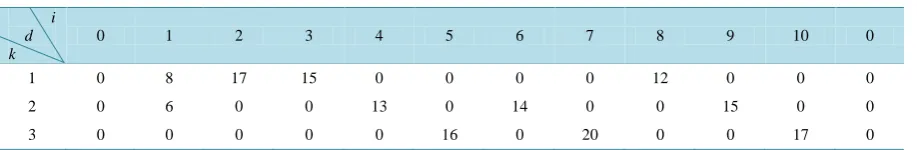
The amount of refined oil distributed for each gas station is shown inTable 6.
Next, according to the heuristic algorithm coded by Matlab software, we obtain an approximate optimal dis-tribution route for 3 tankers: 0-1-3-2-8-0; 0-1-4-6-9-0; 0-7-5-10-0.
The arrival time of each tanker to the gas station is shown inTable 7.
FromTable 7, we can learn that the working time of tanker 1 is 2.21 hours, which of tanker 2 is 2.42 hours
and that of tanker 3 is 2.37 hours. The maximum working time is 2.42 hours, which means the optimal solution obtained by heuristic algorithm is 2.42 hours.
The amount of refined oil per tanker distributed for each gas station is shown inTable 8.
Table 5.The arrival time of each tanker to the gas stations (unit: hour).
i r k
0 1 2 3 4 5 6 7 8 9 10 0
1 0 0.4 0 0 0.86 0 1.42 0 0 1.88 0 2.42
2 0 0 0 0 0 1.75 0 1.18 0.6 0 0 2.42
3 0 0.4 0.82 1.15 0 0 0 0 0 0 1.75 2.42
[image:7.595.86.542.321.397.2]i indicates the gas station; r represents arrival time; k refers to the tanker.
Table 6. The amount of refined oil distributed for each gas station (ton).
i d k
0 1 2 3 4 5 6 7 8 9 10 0
1 0 9 0 0 13 0 14 0 0 15 0 0
2 0 0 0 0 0 16 0 20 12 0 0 0
3 0 5 17 15 0 0 0 0 0 0 17 0
i indicates the gas station; d represents distribution quantity; r refers to the tanker.
Table 7.The arrival time of each tanker to the gas stations (hour).
i r k
0 1 2 3 4 5 6 7 8 9 10 0
1 0 0.4 1.26 0.96 0 0 0 0 1.75 0 0 2.21
2 0 0.4 0 0 0.86 0 1.42 0 0 1.88 0 2.42
3 0 0 0 0 0 1.03 0 0.46 0 0 1.70 2.37
i indicates the gas station; r represents arrival time; k refers to the tanker.
Table 8.The amount of refined oil distributed for each gas station (ton).
i d k
0 1 2 3 4 5 6 7 8 9 10 0
1 0 8 17 15 0 0 0 0 12 0 0 0
2 0 6 0 0 13 0 14 0 0 15 0 0
3 0 0 0 0 0 16 0 20 0 0 17 0
i indicates the gas station; d represents distribution quantity; k refers to the tanker.
5. Conclusions
The inventory routing problem is the key problem in making the distribution plan of the refined oil. The working time equilibrium of each tanker often needs to be considered in the actual arrangement of the oil delivery scheme. In this paper, we study the inventory routing problem, which is to make the working time equilibrium of the tanker as far as possible. The mathematical model of the problem is established and Lingo program is written for solving the model. We further design a heuristic algorithm to solve the problem quickly. The model and algorithm in this paper provide a theoretical basis for the formulation of the oil distribution plan.
[image:7.595.87.546.434.509.2]Acknowledgements
This work was supported by the National Natural Science Foundation of China (11131009, 71540028, F012408), the Funding Project for Academic Human Resources Development in Institutions of Higher Learning under the Jurisdiction of Beijing Municipality (CIT & TCD20130327), and Major Research Project of Beijing Wuzi Uni-versity. Funding Project for Technology Key Project of Municipal Education Commission of Beijing (ID: TSJHG 201310037036); Funding Project for Beijing Key Laboratory of Intelligent Logistics System; Funding Project of Construction of Innovative Teams and Teacher Career Development for Universities and Colleges Under Beijing Municipality (ID: IDHT20130517); Funding Project for Beijing Philosophy and Social Science Research Base Specially Commissioned Project Planning (ID: 13JDJGD013).
References
[1] Herer, Y.T. and Levy, R. (1997) The Metered Inventory Routing Problem, an Integrative Heuristic Algorithm. Interna-tional Journal of Production Economics, 51, 69-81. http://dx.doi.org/10.1016/S0925-5273(97)00059-5
[2] Clauclia, A., Nicola, B., StafanIrnich, M. and Grazia, S. (2014) Formulations for an Inventory Routing Problem. In-ternational Transactions in Operational Research, 21, 353-374.
[3] Vansteenwegen, P. and Mateo, M. (2014) An Iterated Local Search Algorithm for the Single-Vehicle Cyclic Inventory Routing Problem. European Journal of Operational Research, 237, 802-813.
http://dx.doi.org/10.1016/j.ejor.2014.02.020
[4] Li, K.P., Chen, B., Sirakumar, A. and Wu, Y. (2013) An Inventory-Routing Problem with the Objective of Travel Time Minimization. European Journal of Operational Research, 236, 936-945. http://dx.doi.org/10.1016/j.ejor.2013.07.034
[5] Li, X. (2007) Research on Model and Algorithm of Vehicle Routing Problem. Shanghai Jiao Tong University, Shang-hai, 91-105. (In Chinese)
[6] Jiang, B. (2010) Research on Vehicle Routing Problem with Time Windows Based on Genetic Algorithm. Beijing Jiaotong University, Beijing, 8-44. (In Chinese)
[7] Zhao, D., Li, J., Ma, D. and Li, Y. (2014) Optimization Algorithm for Solving Stochastic Demand Inventory Routing Problem with Hard Time Window Constraints. Operations Research and Management Science, 23, 27-37. (In Chinese) [8] Milorad, V., Dražen, P. and Branislava, R. (2014) Mixed Integer and Heuristics Model for the Inventory Routing
Problem in Fuel Delivery. International Journal of Production Economics, 147, 593-604.
[9] Yan, Q.Y., Zhang, Q. and Torres, D.F.M. (2015) The Optimization of Transportation Costs in Logistics Enterprises with Time-Window Constraints. Discrete Dynamics in Nature and Society, 2015, Article ID: 365367.