Corruption and regulatory burden
Dzhumashev, Ratbek
Monash University, Dept. of Economics
5 May 2008
Ratbek Dzhumashev,
†May 5, 2008
Abstract
It is known that government has discretionary power in providing public
goods and regulating the economy. Corrupt bureaucracy with discretionary
power creates and extracts rents by manipulating with the public good
supply and regulations: i) by attaching excessive red tape to the public
good they are providing; ii) or by making the regulations difficult for the
private agents to comply with. The former type of corruption results in
less public input being provided at higher cost to the private agents. The
latter increases non-compliance, which then breeds bribery. Consequently,
the overall public sector burden is higher in the environment with corrupt
bureaucracy. We show this outcome using a simple theoretical model, and
then confront it with empirical evidence.
∗I thank Prof. Yew-Kwang Ng for the valuable comments on the paper
†Building 11, Department of Economics, Monash University, Clayton, Vic 3800. Email:
1
Introduction
Some researchers find that corruption can play a positive role for economic growth
by decreasing red tape. However, this finding rests on the assumption that
cor-ruption and red tape are independent from each other. In reality, it is a strong
assumption. Both corruption and red tape are created by the same bureaucracy
and thus it is more reasonable to assume that they are dependent on the
charac-teristics of the underlying institutions.
The idea that the inefficient government sector can lead to larger optimal size
of government has been demonstrated by Ng (2000). The increase in government
size implies a heavier public sector burden. In this work I set a task of
relat-ing the public sector burden with the inefficiencies stemmrelat-ing from corruption of
bureaucracy running the public affairs.
The paper in particular aims to develop a simple model that enables to
as-sociate the quality of bureaucracy with the regulation burden. In other words,
endogenous red tape or regulatory burden is modelled as depending on the
qual-ity of public institutions or conversely on the corruption level in them. Then
the proposition stemming from of the model suggesting a positive relationship
between corruption and regulatory burden is tested empirically.
Since we will be referring to the concept of red tape we need to define it first.
In the current context red tape is defined as a set of procedures obligatory to
fulfil by the private agents to obtain public goods and services to operate legally.
In fact, red tape is a type of regulation set and enforced by the government.
The other regulations can be lumped into one non-red-tape regulations group.
with obtaining public good or service.
Corruption is defined as illegal use of public position for personal gain. The
public position provides the power to introduce, implement and enforce
regula-tions and rules. In corrupt environments the discretionary power of the public
officials is strong and their activities are not transparent.
We know that in general the government is a monopolist in the provision
of public goods and services. At the same time the purpose of government is
not profit maximisation, therefore, a benevolent government should provide the
goods and services at their marginal cost.
Corrupt bureaucracy uses its public position for creating and extracting rents
from the private sector. In general, the bureaucracy does it by abusing their
monopolistic power and manipulating with red tape and regulations. Therefore,
the regulations are not independent of corruption, but is a mechanism used by
corrupt bureaucracy to extract rents from private agents.
Shleifer and Vishny (1993) and Barreto (2000, 2003) indicate that corrupt
bureaucrats take advantage of their monopolistic power and rent-seek. The
mo-nopolistic behaviour of the public agents leads to less public goods being offered
to the private sector. As the act of corruption is illegal, the bureaucrats do
not openly increase the price for the service they are providing as the private
monopoly would do. Also any official increase in public good prices leads to an
increase of government revenue, not the corrupt official‘s income. So rent-seeking
is done by simple creation of hurdles or red tape on the way of the private agents
trying to obtain public services and goods. In general, an optimal level of red tape
There-fore, we refer not to red tape in general, but only to its type, which is excessive
and wasteful. For example, corrupt officials tend to create long queues or erect
artificial barriers for the private agents by making up ad-hoc procedures and
requirements.
The time of the bureaucrat is limited, thus engagement in creation of excessive
red tape effectively decreases his useful output. Instead of the costly red tape
the private agents might choose to pay a bribe to the bureaucrat on top of the
statutory cost of the public service or good. That is what usually called “speed
money” or “greasing the wheels”. This is the main reason to see corruption as a
phenomenon improving efficiency by speeding up rigid bureaucracy. However, in
the first place, the bureaucracy become slow and rigid due to corrupt intentions,
as it is how they invite for bribing.
From the corruption literature we know that corruption may happen ex
ante or ex post. In the ex ante corruption or “corruption without theft” the
bureaucracy increases the price of the public goods before the interaction with
the private agent. As the bureaucracy has the monopolistic power it can charge
monopolistic prices for the public goods it is providing. The other example of the
ex ante corruption is framing and extortions exercised by public officials abusing
the public power endorsed upon them.
It is apparent that the institutions of poor quality create opportunities for
the public officials to engage in such corrupt behaviour. Since the higher cost of
obtaining public good or extortions decrease private agents income, the ex ante
corruption increases the burden of the public sector.
bureau-cracy learns about the type of the private agent and can conceal socially valuable
information for private gain. Usually it happens when the corrupt bureaucrat
in-specting the private agent finds that the private agent has not fulfilled his liability
required by regulation.
A regulation may be introduced in order to deal with externalities created by
private production or other social reasons. In case ofex post corruption, both the
inspector and the producer might gain at the expense of the society as a whole.
This type of corruption may decrease the burden of regulations on the individual
agents involved. However, if the enforcer also has the opportunity to set the
regulation parameters then he will increase the effective burden of the regulation,
so that the rent created is fully captured by the bureaucrat. The effective burden
of regulations on the private agents, in this case, does not decrease, though lower
compliance with the regulations increases negative externalities.
Due to increased negative externalities imposed on the other agents,
corrup-tion makes the society as whole worse-off. For example, in some countries traffic
police is so corrupt that one can just buy a drivers’ license and pay off his way in
case of violating traffic rules. Seemingly it should make the individuals life easier,
but as everybody on the road is doing the same, driving becomes a formidable
experience. In fact, the indirect burden of such corruption is much higher than
its direct burden.
Summing up, we can state that the driving force of corruption is the possible
rents that may be captured by the bureaucracy. The rents can be created only
through regulatory power of the government, thus regulatory burden is directly
can conjecture that corruption and red tape (regulation burden) are correlated
and both depend on the deeper parameters characterising the public sector.
This paper contributes to the literature by constructing a model that relates
the quality of institutions to the burden of the regulations. The results leading
to this conclusion are based on both a theoretical model and empirical tests on
the validity of the hypothesis stemming out of the theoretical model.
In the theoretical model the government provides a single public good. We
assume that this good is an essential input to private production. We relate
the benevolence measure of the bureaucracy to its capacity to reap
monopo-listic rents in providing public goods. The bureaucracy also sets and enforces
externality-related regulations. The bureaucracy increases statutory burden of
the regulations by manipulating with the regulation parameters. The high
bur-den of the artificially stringent statutory regulation decreases compliance rates
among the private agents as they seek their way out by bribing the bureaucrats
involved. We show that in such an environment under some conditions with the
increase of corruption the equilibrium regulation burden becomes higher.
To test the prediction of the model we formulate a hypotheses stating that the
corruption level and governance quality are associated and there is positive
corre-lation between the measure of corruption and the effective cost of red tape. Using
cross country data we find strong dependence between the corruption measure
and the governance measures that reflect the quality of the public institutions.
The second hypothesis postulating a positive association between the corruption
level and the regulatory burden is tested, and the evidence supports the
The paper is organised as follows. First I set up a theoretical model and
find its solution. Then I test the main hypothesis that whether the level of
corruption is associated with the quality of underlying institutions; and whether
the countries with higher corruption levels also have a higher red-tape burden? In
the last section I draw conclusions about how corruption and regulatory burden
are related.
2
A review of the literature
In the literature there are conflicting views about the effect of corruption on
economic efficiency. Basically, there are findings that corruption can be
effi-ciency enhancing in the over-regulated, rigid and inefficient environment. To
the best of my knowledge, since Leff (1964) the idea that corruption contributes
to efficiency improvements has find its proponents. Leff (1964) advocates
cor-ruption on the grounds that it helps to circumvent bad regulations and thus
improves economic efficiency. A similar rationale is used in arguments presented
by Huntington (1968), Tanzi (1998), Kaufmann and Wei (1999), Barreto (2000);
Barreto and Alm (2003). They point out that corruption can help to overcome
different regulatory obstacles and lessen the adverse effect of bad policies and
governance.
Meon and Weill (2006) find some evidence supporting the hypothesis that
corruption can be efficiency-enhancing. They claim that corruption is positively
related to the efficiency in countries with malfunctioning institutions. Though,
they find that in countries with effective institutions the relationship between
The other argument used to support the efficiency-enhancing nature of
cor-ruption is that it leads to better resource allocation. In other words, corcor-ruption
functions similar to auctions that determine the most efficient allocation of the
public goods, permits, and licenses. According to this argument corruption allows
distributing permits to most efficient producers and lowers regulatory burden at
the same time (Lui, 1985).
This argument is based on the implicit assumption that the public power is
exogenously given to the public officials. The reality is much more complicated
and public officials in corrupt environments are not independent agents but a
members of some clans or groups. So they are not totally driven by their
indi-vidual short-term interests, but to keep their own rent seeking position in the
long-term they serve the clan’s interest which they are a member of. In other
words, corruption cronysm, nepotism and patronage go along with corruption in
the public sector. Therefore, there is nothing like auctions in distribution of
per-mits and licenses. It is rather a distribution of perper-mits driven by the combination
of short-term and long-term rent-seeking.
The other view is that corruption may improve professional quality of the
public officials as it creates incentives to attract talents by increasing their
ef-fective incomes (Bailey, 1966; Leys, 1965). However, this only makes corruption
schemes more sophisticated and harmful, as there is no guarantee that more
talented people are less self-interested.
Nevertheless, the contemporary dominating view is that corruption is a
sig-nificant impediment for economic growth. The main argument is that the
to corruption. Corrupt bureaucrats create those regulatory barriers to extract
bribes from the private agents (Myrdal, 1968). Corruption may increase
num-ber of transaction with the bureaucracy, which offsets any efficiency gains from
corruption (Bardhan, 1997; Jain, 2000; Kaufmann and Wei, 1999). In addition,
corrupt bureaucrats create distortions in the public and private sectors to create
rents or just to maintain them (Kurer, 1993; Mauro, 1995; McChesney, 1997;
Shleifer and Vishny, 1993; Tanzi, 1998). The empirical studies by Mauro (1995),
Brunetti et al. (1998), Mo (2001), and Ali and Isse (2003) confirm the negative
relationship between corruption and growth.
Barro (1990) and Keefer and Knack (2002) show that when government is
rent seeking the overall public burden increases. Their result indirectly supports
the idea that corrupt bureaucracy is positively correlated with a higher regulatory
burden. Modelling the interaction between the corrupt bureaucracy and private
agents, Guriev (2004) finds that in the corrupt environment the equilibrium
bur-den of red tape is higher than in the absence of corruption. His model is based
on the agency theory, and assumes heterogeneous private agents of two types.
However, there is no quality measure for the bureaucracy in his model that can
be related to the level of corruption in the economy.
The literature, with the exception of Guriev (2004), lacks studies of the
de-pendence between corruption level and regulatory burden. To the best of our
knowledge there has not been any empirical study testing the correlation
be-tween corruption and regulatory burden. The aim of the paper is to address this
3
The model
3.1
Assumptions
Let us first lay out our assumptions about the agents operating in the economy,
their preferences, and production technology.
3.1.1 The Agents
Suppose that the model economy is populated with identical household-producers
and bureaucrats. Each private agent has an initial endowment of consumer goods
of X. If the agent decides to produce, he has to obtain public input essential for
production. This condition captures the public sector involvement in production
through permits, licenses, certifications, and provision of infrastructure and other
public inputs.
The agents preferences are defined by a utility function of the form:
u=u(y, e) (1)
where y is income, e is the quality of the environment the agents living in. I
use income as an argument of the utility function n as we are assuming away
saving in our model. I also assume that the utility of the agent is increasing in
both arguments, u′
y, u′e > 0. The environment measure depends on the hazard
or negative externality in general, h. From now I refer to this variable as the
externality. Put it formally as e = e(h), e′(h) < 0, where h is a measure of the
externality stemming from production process.
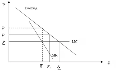
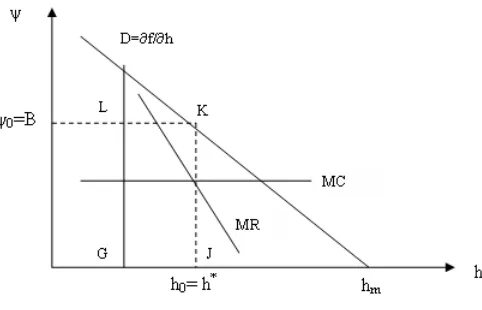
qual-Figure 1: Public good provision in a corrupt environment
ity measured by an indexI ∈[0,1]. Only if I = 1, the bureaucracy is completely
honest and benevolent.
The government provides public goods that are essential input to private
production. The fully benevolent bureaucracy provides the public good at its
marginal cost, however, when the bureaucracy is not fully benevolent or when
I <1 the price of the public good is set with a mark-up.
p=M C + (1−I)m (2)
where M C is the marginal cost of public good production, m is the maximum
mark-up. The second term in this equation is the cost of corruption imposed on
the private agents.
This model is in fact, an extension of the model proposed by Shleifer and Vishny
[image:12.595.189.437.135.286.2]de-termined from the profit maximisation and given by curve D in Figure 1. The
price for the public good is defined on p ∈ [p,p¯] , where p = M C is the legal1
price set by the government, while ¯p=M C+mis the higher price acceptable by
producers. The price faced by the private agents is higher with higher corruption
as I <1 implies p > p.
Note, in any case the bureaucrat reports the legal pricep, while any exceeding
amount per unit of the public good equal to pc−p is pocketed by him. We can
treat the mark-up as a bribe paid by the private agent to obtain the public
good. We assume that the bureaucracy is paid salary w equal to the sum of two
components. Formally it is expressed as
w=pg+ ¯w (3)
where g is the real amount of the public services provided, ¯w is the salary of the
bureaucrats independent of their efforts at work.
In reality, it is possible that the bureaucrats get only a fraction of the revenue
pg as a salary. For simplicity we assume that they get all the revenue as their
salaries. Thus with the bribes the bureaucrats‘ actual income equals
wb =w+ (1−I)ms1 (4)
wheres1 is the productivity of the public official. To make our algebra simple we
assume that s1 = 1.
1We are assuming that at least at the political level government is instituted for promoting
3.1.2 Private Production
The private agent might spend a portion of his endowment X to buy the public
good and engage in production. His production technology is given by
ya=f(g,¯l, h). (5)
where, g is the real amount of public inputs, ¯l is the fixed amount of labour,
and h is the hazard to environment created or generally the negative externality
of production. That is to say that the quality of environment e is a function
of this production externality h, or e = e(h). Note, without obtaining the
pub-lic good the production process does not take place. We assume the
produc-tion funcproduc-tion f(g,¯l, h) is continuous and monotonically increasing ing and h, or
lim
g,h→0f
′
g(•), fh′(•) =∞ and limg,h→∞f
′
g(•), fh′(•) = 0 and f
′′
g(•), fh′′(•)<0. Here and
further • denotes all other arguments of a function.
The producers maximise their profits treating the institutional structure and
technology as given. This problem is formally stated as:
max
g,h y=f(•)−c1(g)−c2(h) (6)
where c1(g) =pg is the cost of the public input,c2(h) = ψ(h−h0) is the cost of
the externality exceeding the allowed limit.
The first-order condition with regards to the public input for this problem
leads to the optimality condition for the private agent:
pc =
∂f(•)
where pc is the equilibrium price of the public input provide by the monopolist
bureaucrat.
Recall that the rent seeking public officials charge higher prices for the public
input they are providing, or pc > p. Denote by ¯g the amount of public input
obtained by the producer at the minimal price p. Based on the condition in (7)
and the properties of the production function (f′
g(•)>0,fg′′(•)<0), we infer that
gc <g¯, wheregcis the amount of the public input. Since the production function
is increasing in the public inputg, the following conditionf(gc,•)< f(¯g,•) holds.
Therefore,we conclude that in a corrupt environment private output is lower than
in the absence of corruption, other inputs being the same.
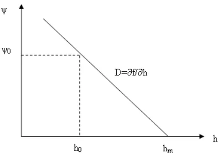
3.1.3 Production Externality
The level of the negative externality created by production process, h, can be
chosen by the producer based on his technology, ya = f(g, h,¯l). Suppose that
the level of h that maximises f(•, h) is equal to hm. However, this level of
externality may not be acceptable for the society. In this case the government
establishes a regulation that sets a ceiling to the permitted level of the externality
as h0 < hm.
To maximise their profits the producers choose the externality level h given
the probability of being caught and punished.
The FOC of (6) with regards to h yields us the following:
∂f
∂h −ψ = 0 (8)
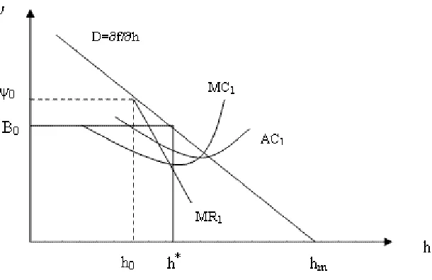
Figure 2: Full compliance in the absence of corruption
h∗.
The price of the excessive externality depends on the penalty rate of
non-compliance, φ and the probability of detection, δ. Thus we can write, ψ = δφ.
The benevolent government chooses δ and φ in such a way that it would be
optimal for the producer to comply, or
ψ0 ≥ ∂f
∂h|h∗=h0
whereh∗ is the optimal amount chosen by the producer,h
0is the officially allowed
level of externality.
This outcome is illustrated in Figure 3. When the cost of the externality
is equal to ψ0 the producer will choose not to demand h in excess of the level
permitted by the regulation. Therefore, in this case the producer complies with
the regulation and demands only the free allowance equal to h0.
Figure 3: Corruption with theft
prices. The corrupt bureaucrats can sell the additional allowances for externality
at lower price, B0, which is just the bribe rate.
Usually, government regulations are enforced by a specific department or office
depending on the nature of the regulation. Also the bureaucracy one has to deal
with is also location specific, so that if one has a business in some location then
the entrepreneur is attached to a certain local bureaucracy in terms of regulation
compliance. Put in another way, the bureaucrats exercise monopolistic power in
provision of public services and regulation enforcement.
As a monopolist the bureaucracy supplies the additional externality allowances
in the amount that equalises its marginal revenue M R1 and marginal costM C1.
Note, that the effective demand by the producers for additional externality starts
only after pointh0. Therefore, the marginal revenue curveM R1 is effective only
The bureaucrats face some costs when they allow for excessive externality.
The cost schedule faced by the corrupt bureaucrats can be non-linear in general
as it is depicted in Figure 3. However, for simplicity we can assume that this
cost is a function of the amount of the excessive externality being sold by the
bureaucrat. So, this cost is given as as the following function:
cb =γ0(h−h0) (9)
where γ is a cost parameter. Given the cost function the bureaucrats then
max-imise their net bribes. In this setting the marginal cost then is given by:
M C1 =c′
b(h) =γ0
The result of such a corrupt interaction should be higher equilibrium
exter-nality equal to h∗ > h0, which is depicted in Figure 3.
Since only those who do not comply with the regulation are subject to
bribe-paying, it is in the corrupt bureaucrats’ interest to have more violators among the
producers. The simple way to do that is to make the regulation more stringent
by decreasing the allowed level of externality. In our context, it is equivalent to
decreasing the allowed ceiling for externalities from h0 tohc < h0.
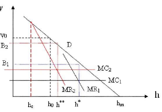
The implications of such corruption is illustrated in Figure 4. Now the corrupt
bureaucrats can sell more allowance of externality than before. Therefore, they
now have a new marginal revenue curve given by M R2. However, this type of
corruption involves violation of more laws than just the corruption with theft,
Figure 4: Combination of corruption with theft and without theft.
In the simplest setting the cost faced by the bureaucrats should have two
components. The first component should capture the cost for taking bribes that
is related to the amount of externality, whereas there should be cost related to
the extortionary behaviour of the bureaucrats. Based on this rationale we assume
that the cost of the corrupt bureaucrats is given by
cb = [γ0+γ(h0−hc)] (h−hc) (10)
Under this condition marginal cost curve is given by
M C2 =c′b(h) = γ0+γ(h0−hc) (11)
It is clear that the marginal cost of the corrupt bureaucrats is greater in these
circumstances, as M C2 > M C1 = γ0. The equilibrium externality level is then
Figure 5: Extortionary corruption
than in the case without extortions, B2 > B1. The results of the analysis are
illustrated in Figure 4.
Based on the logic of this model we can find that it is possible the bribe
level is equal to the official cost of non-compliance, B =ψ0, and the equilibrium
externality allowed is equal to the officially allowed level,h∗ =h0. However, this
allowed externality level is not obtained free of charge as in the case without
corruption, but rather involves a burden of bribing the corrupt officials. This
outcome is portrayed in Figure 5. The burden of corruption here is the cost of
bribes measured by the area of rectangle GLKJ.
The other important question is: what is the equilibrium level of the allowed
externality set by the corrupt bureaucracy, hc? The corrupt bureaucrats
max-imise their bribes given the cost they face for being corrupt. As we supposed
earlier, the higher extortions are made by deviating more from the legal
bench-markh0. However, the greater the deviation from the legal benchmark, the higher
bribes, R, by taking account of the possible costs:
max
hc
R=
Z h
hc
(B−AC)dh,
s.t.M R=M C
whereB is the bribe rate, AC is the average cost of selling a permit for a unit of
externality, h0 is the legal benchmark for externality, hc is the lower benchmark
set by corrupt bureaucrats.
For illustration purposes we consider a specific case. Suppose that the bribe
obtained per unit of excessive externality is given by
B =b0+b(h0 −hc).
This formulation captures the idea that the lower the benchmark set by the
corrupt bureaucracy for free externality, hc, relative to the legal benchmark, h0,
the higher the bribe rate.
Suppose, the average cost of corrupt bureaucrat is given by
AC = cb
h−hc
=γ0+γ(h0−hc).
From condition M R = M C we get the optimal demand for h∗. Then taking it
into account we can state the bureaucrats problem as
max
hc
The FOC with respect to hc is then given by
(b0−γ0+ (b−γ)(h0−hc)−(b−γ)(h∗−hc) = 0.
By solving forhc we obtain its equilibrium value
h∗c = (h
∗ −h0)
2 −
b0−γ0
2(b−γ) (12)
From this result we can infer that an increase in rents from corruption with
theft (b0−γ0) relative to the rents from predation (b−γ) leads to higher predation,
defined as a lower value for h∗
c. So policy-wise it is more effective to focus on
curtailing the corruption with theft, which also decreases predatory behaviour of
the bureaucracy.
We also infer that the corrupt bureaucrats set the allowed level of the
exter-nalityhcsuch that the condition given by h∗ > h0 holds. Put another way, in the
environment with corrupt bureaucracy, the equilibrium level of the externality
exceeds the legally permitted level.
3.2
Welfare implications
If there was no restriction on the externality then the producer would use hm at
no charge. However, the regulation sets the allowed externality equal toh0, which
is also free of charge. Then for the individual producer who does not take into
account his contribution to the quality of environment, the effect of the regulation
equals the foregone output.
per-mitted hazard or externality can be found as a difference between the maximum
output in case of no regulation,ym =f(•, hm), and the optimal output under the
regulation, y=f(•,h0¯). This condition is captured by
T0 =f(•, hm)−f(•, h0) (13)
The utility of the agent also depends on the quality of the environment, and
due to regulation the environment is improved by e(h0)−e(hm), where e(h0)>
e(hm). So, the overall effect of the regulation depends on whether utility decreases
Ua[f(·, hm), e(hm)]> Ua[f(·, h0), e(h0)]
or increases
Ua[f(·, hm), e(hm)]< Ua[f(·, h0), e(h0)]
is true. It is reasonable to assume that the benevolent government chooses the
regulation in a manner that improves the overall welfare, so that the latter
in-equality holds.
In case of corruption with extortions the effect of the regulation on the
pro-ducer is then given by
Tc=
£
f(•, hm)−f(¯l, gc, h∗)
¤
+B(h∗−hc) + (pc−p¯)gc (14)
where the last terms stand for the amount of bribes and the surcharge for the
public input correspondingly.
producer in the environment with corrupt bureaucracy is strictly higher,
Tc > T0
Then we can ascertain that in this case the overall welfare effect of corruption is
negative, and expressed as:
Ua
£
f(¯l,g, h0¯ ), e(h0)¤
> Ua
£
f(¯l, gc, h0)−B(h0−hc)−(pc−p¯)gc, e(h0)
¤
Earlier, for the specific form of the cost function we found that the equilibrium
externality is greater than the legal level h∗ > h0. However, with corruption the
public input is lower, or gc<¯g. Then the burden of regulation can still be higher
than the legal one. In other words, as soon as the condition
f(¯l,¯g, h0)> f(¯l, gc, h∗)−B(h∗−hc)−(pc−p¯)gc
holds, Tc > T0 is also true. Recall that h∗ > h0 implies e(h∗) < e(h0). Thus
this outcome suggests that due to corruption the private agent may loses both in
income and in the quality of the environment.
This is then the worst social outcome as the producers face higher costs in
obtaining the public input and the negative externality is higher than the optimal
level. Also note that the bribes paid by the private agents are not fully transferred
to the bureaucracy as they waste resources while extorting bribes reflected by the
cost of rent seeking, cb. The overall effect then will be a loss incurred to social
The other implication we may consider is that the concept of environment
can be considered from a wider perspective and by going beyond the natural
environment. The wider concept of environment may also include the safety
and property rights protection. So the increase in the externality level may also
affect the efficiency of the production process. As in the example of the traffic
rules being enforced by the corrupt officers mentioned earlier: the increase in
externality due to corruption may lead to strong deterioration of the environment.
In such a case the personal gain from non-compliance is offset entirely by the
adverse effect of the negative externality imposed by others.
This logic can apply in general: as the government fails in its organising role
and boosting cooperation, the private agents may find themselves in an uncertain
environment with high levels of negative externality. This should imply higher
cost for production, safety, property rights protection, which leads to lower output
for any given level of inputs.
Summarising we draw the following conclusions:
1. Corruption increases the direct burden on the private agents
• from the condition that the bureaucrat maximises his revenue we
con-clude that the condition pc> p the cost of the public inputs is higher
with corruption,
• in addition to it, the corrupt bureaucracy increases red tape related
to the externality standards thus making the cost of the regulation
heavier. The effective burden of regulations, when the bureaucracy
is corrupt, can exceed the burden, when bureaucrats are honest, or
2. Corruption creates inefficiencies that lead to lower aggregate income and
poorer quality of the environment. This may result in overall welfare loss.
It is a standard approach to define the public sector burden as a ratio of the
cost of the burden to the total income. In the absence of distortions caused by
tax evasion and corruption, the public sector burden is given by
τ = T0
Y ,
whereτ is also the statutory tax rate. In the presence of tax evasion and
corrup-tion, the public sector burden is different, as we see above. Applying the same
logic, we can write the relative burden as
τe =
Tc
Y ,
whereτe is different from the statutory tax rate,τ. In case,Tc≥T0 is true, then
τe≥τ should hold. Importantly, this result also shows that corruption alters the
effective public sector burden.
The analysis based on the theoretical model has shown that with broader
corruption, that not only lets for lower compliance with the regulations, but also
makes the regulations harder to comply with, can result in overall heavier public
sector burden. Based on this rationale we formulate the following proposition,
which will be tested empirically in the next section.
4
The empirical analysis
4.1
Hypotheses
Based on the theoretical model we state two hypotheses to test:
H1: The level of corruption depends on the quality of the public institutions
H2: The regulatory burden in the economy is positively associated with the level of corruption.
The first hypothesis captures the assumption of the theoretical model that
relates the level of corruption to the quality of the institutions. That is, I am
assuming some sort of functional relation between the corruption level and the
quality of the public institutions given as
CP I =̥( quality of public institutions)
The empirical model that spells out this relation can be stated as
CP Ii =α+βZ+εi (15)
where CP Ii is the measure of the corruption level, Z is a vector of measures of
the quality of governance,εi is the disturbance term.
The second hypothesis is based on the idea that corruption changes the
effec-tive burden of the public sector. By comparing (14)Tc=
£
f(•, hm)−f(¯l, gc, h∗)
¤
+
B(h∗−h
c) + (pc−p¯)gcand (13)T0 =f(•, hm)−f(•, h0) we can easily state that
corruption captured by the values of the parameters such as the bribe rate, the
levels of public sector burden. Therefore, the effective public sector burden can
be represented as a function of corruption,
Tc=̥(corruption measure, Y, τ), (16)
where Y is the total income, τ is the statutory public sector burden. In other
words, for given total income and regulation parameters, the effective public
sector burden can differ depending on the corruption level in the economy. One
may ask, if corruption causes high public burden? We do not know yet. However,
corruption certainly changes the burden, and we have discussed the intuition.
To test the second hypothesis we write on the basis of (16) our empirical
model as
burdeni =α+βCP Ii +bX+εi (17)
whereburdeni is a measure of the effective regulatory burden for a given country,
α is a constant term, β is the coefficient at the measure of corruption CP Ii for
the country,Xis a vector of other variables that may be included into the model,
εi is the disturbance term. Note, empirically we cannot claim that corruption
causes changes in the statutory burden, as we do not know the magnitudes of
the statutory burden. Instead, we claim, that the corruption leads to changes in
the effective or observed public sector burden. The theoretical model shows this
relation.
To sum up, if we cannot reject the first hypothesis that will support the idea
that corruption is endogenous to the institutional structure of the economy. If
corruption does not lead to efficiency improvements through reduction of red
tape.
4.2
Data description
The data set constructed for the empirical analysis in order to find dependence
between corruption and regulation burden consists of cross-country data for 140
countries (for 2005). The list of variables with description is given in the
ap-pendix.
There are three types of data we use in the analysis.
1. A measure of corruption,
2. Measures of institutional quality or governance,
3. Measures of regulation burden.
4.2.1 Corruption measure
The level of corruption is measured by an index, and in our case we employ
the Corruption Perception Index (CPI) complied by the Transparency
Interna-tional. This measure of corruption is based on the surveys of the private agents
perception of corruption related to their economic activities, hence is called the
Corruption Perception Index. The CPI values are determined in the range of
(0, 10), the higher value signifies the less corruption in the economy. We
trans-form the original variable CPI to CI = 10−CP I , so to associate higher values
with higher corruption. For comparison reasons we also use a variable named
control” values are determined in the range of (-1.5, 2.5), again the higher values
signify the better corruption control in the economy. The data for this variable
is extracted from the Governance Indicators Dataset (Kaufmann et al., 2004).
4.2.2 Governance
The quality of institutions is represented by Governance Indicators Dataset
com-plied by the World Bank. These measures include indexes (ranges are indicated
after each index) on Government effectiveness (GE ∈ (−2,2.5)) , Rule of Law
(ROL∈(−2,2.5)) , Regulatory quality (REG∈(−2,2.5)) , Voice and
Account-ability (VA ∈(−2,2)) , Political stability (PS∈(−3,2.5)) .
4.2.3 Regulation burden
The cross-country data on the burden of regulations were obtained from the
database “Doing Business” compiled on the base of the World Business
Environ-ment Survey. The data from the Doing Business database includes the measures
of costs related to different regulations and activities. The costs of regulations
are pegged to the per capita income of the given country and also given as time
spent on dealing with the regulation. In this analysis I use only comparable
costs in real terms, that is the cost in terms of time spent on meeting the
reg-ulations. Specifically, the following cost measures are used: Starting a business
cost (days), Dealing with licences cost (days), Property registration cost (days),
Tax payment cost (days), Export operations cost (days). I actually use a sum of
with, RTCOST , is found as
RTCOST = Starting a business cost +
+Dealing with licences cost+
+ Property registration cost
+Tax payment cost + Export operations cost
(18)
On the base of the different costs related to doing business, the countries
are ranked and the aggregate index called the “Ease of Doing Business Rank” is
constructed by the World Bank. The “Ease of Doing Business Rank” measures
overall burden of regulations on the businesses and denoted as DBR. The easier
is the burden the higher is the rank.
4.2.4 Macroeconomic data
In order to control for the income effect, the data on the GNI per capita in US
dollars were obtained from the World Development Indicators database. The
intuition behind the idea of using the income differences as a factor affecting
the regulatory burden is as follows: It is quite intuitive to assume that higher
income is associated with higher productivity, more complex technology and
eco-nomic structure. The advanced technology and complex structure of the economy
must involve greater regulation and therefore, the regulation burden should be
4.3
Data Analysis
4.3.1 Hypothesis on corruption and the quality of the public institu-tions
To see if the corruption level of the country is associated with its governance
indicators we explore the data for corruption level and governance. The simplest
way to do is to determine the correlation coefficients between the Corruption
Index (CI) and the other governance indicators.
The Jarque-Bera test statistics for corruption measures, CPI and CI,
demon-strate a departure from normality. Therefore, to account for non-normality we
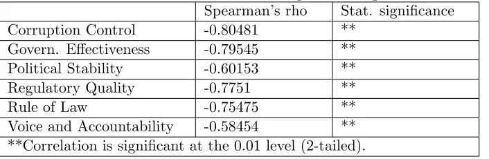
find Spearman’s rho between CI and the governance indicators. The results are
given in Table 1. We see that all governance indicators manifesting the
underly-ing institutional quality are negatively and strongly correlated with the level of
[image:32.595.109.462.485.600.2]corruption. It is also evident from the Kendall-plots given below in Figure 6.
Table 1: Correlation between corruption and governance measures
Spearman’s rho Stat. significance Corruption Control -0.80481 **
Govern. Effectiveness -0.79545 ** Political Stability -0.60153 ** Regulatory Quality -0.7751 ** Rule of Law -0.75475 ** Voice and Accountability -0.58454 ** **Correlation is significant at the 0.01 level (2-tailed).
4.3.2 Kendal-plots
Kendall-plot (Genest and Boies, 2003) are based on the probability integral
pos-sible dependence between variables. We use these plots to identify the pospos-sible
dependence between corruption and governance measures.
The Kendall-plot (K-plot) also depends on the ranks of the data. It is
ob-tained in the similar fashion as a QQ-plot. AssumeH is a bivariate (continuous)
distribution function. The pairs (Xi, Yi) are transformed to pairs (Wi:n, H(i)) for
i=1,2,...n, where H(i) values are ordered according to: H(i) < ... < H(n). These
values are order statistics related to the quantities H1, ..., Hn that are calculated
as
Hi =
X
j6=i
I(Xj ≤Xi, Yj ≤Yi)/(n−1) (19)
TheWi:nvalues are expectations of theithstatistic from the random sample of the
random variable W = C(U, V) =H(X, Y) of size n. Under the null hypothesis
U and V (or X and Y) are independent. The Wi:n values can be calculated as
follows:
Wi:n=ωko(ω){Ko(ω)}i−1{1−Ko(ω)}n−idω (20)
where Ko(ω) =P(U V ≤ω) =P(U ≤ υω)dυ= 1dυ+ ωυdυ=ω−ωlog(ω) and k0
is the corresponding density.
I have constructed K-plots (Figure 6) for pairs that include corruption
per-ception index (CPI) and governance indicators as governance effectiveness (GE),
regulatory quality (REG), rule of law (ROL), voice and accountability (VA),
po-litical stability (PS), and overall measure of regulatory burden–Doing business
rank (DBR).
Recall that if two variables are independent, then the K-plot will be a straight
Figure 6: K-Plots for corruption and governance measures
0 0.5 1
0 0.2 0.4 0.6 0.8 1 H(i)
CPI and DBR
0 0.5 1
0 0.2 0.4 0.6 0.8 1
CPI and GE
0 0.5 1
0 0.5 1
H(i)
CPI and REG
0 0.5 1
0 0.5 1
CPI and PS
0 0.5 1
0 0.2 0.4 0.6 0.8 1 Wi:n H(i)
CPI and VA and va
0 0.5 1
45-degree lines indicates the dependence between the variable. We also can infer
that the sign of the association between the variables are persistent. One can see
that there is strong positive dependence between CPI and all other governance
indicators, whereas, CPI and regulatory burden (DBR) have a negative
depen-dence. The empirical evidence supports our conjecture about the association
between the quality of institutions and corruption, and corruption and
regula-tory burden. Unfortunately, the lack of time series for the given variables does
not allow us to consider causality issues between the levels of regulatory burden
and corruption measures.
4.3.3 Regression results: Hypothesis I
The OLS estimation of the general equation relating the corruption index with
governance indexes, CIi =α+βZ+εi , where Z ={ Government effectiveness,
Corruption control, Regulatory quality, Rule of law, Political stability, Voice and
Accountability } is given as:
CIi =C1+C2CCi+C3GEi+C4REGi+C5ROLi+C6PSi+C7VAi+εi (21)
The model explains almost 81% of variation in the corruption measure across
the countries. Although only the coefficient at CC and the constant term are
significant. The diagnostic test for heteroscedasticity shows that the variance
is constant. The RESET test indicates that the following types of specification
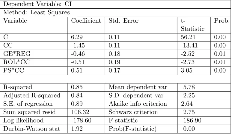
Table 2: Regression results: CI vs. Governance measures with interactions
Dependent Variable: CI Method: Least Squares
Variable Coefficient Std. Error t-Statistic
Prob.
C 6.29 0.11 56.21 0.00
CC -1.45 0.11 -13.41 0.00
GE*REG -0.46 0.18 -2.52 0.01 ROL*CC -0.51 0.19 -2.73 0.01
PS*CC 0.51 0.17 3.05 0.00
R-squared 0.85 Mean dependent var 5.78 Adjusted R-squared 0.84 S.D. dependent var 2.25 S.E. of regression 0.89 Akaike info criterion 2.64 Sum squared resid 106.32 Schwarz criterion 2.75 Log likelihood -178.60 F-statistic 186.90 Durbin-Watson stat 1.92 Prob(F-statistic) 0.00
By trying different functional forms we obtain the following model
CIi= C1+C2CCi+C3(GEi·REGi) + C4(ROLi·CCi) + C5(PSi·CCi)+εi (22)
This model passes both heteroskedasticity and RESET tests, and is better in
terms of Log likelihood, AIC and Schwarz criterion. The signes at CC
(Corrup-tion Control) , and the interac(Corrup-tion terms GE*REG (Governance efficiency and
Regulation quality), ROL*CC (Rule of Law and Corruption Control) is negative
as expected (see Table 2). The interaction term PS*CC (Political Stability and
Corruption Control) has a positive sign, which a bit surprising. A possible
expla-nation as it is argued by Olson (1984) is that in stable societies the bureaucracy
can be more rent-seeking.
Table 3: Correlation between corruption and regulatory burden
Spearman’s rho
CI CC DBR RTCOST
CI 1.00 -0.80 0.66 0.55 CC -0.80 1.00 -0.73 -0.61 DBR 0.66 -0.73 1.00 0.76 RTCOST 0.55 -0.61 0.76 1.00 **Correlation is significant at the 0.01 level (2-tailed).
governance indicators that measure quality of the underlying institutions and the
corruption level represented by the corruption index CI. Much of the variation
in corruption level can be explained by the differences in governance indicators.
Therefore, our first hypothesis is not rejected.
4.3.4 Hypothesis on corruption and regulation burden
The next step is to test the second hypothesis. Again we start with a simple
correlation analysis. The Spearman‘s rho between two regulation burden
mea-sures and corruption meamea-sures are given in Table 3. First we see that there is
a strong correlation between the regulation burden measures given by “Ease of
Doing Business Rank” or DBR, and our computed time burden indicator
RT-COST. The corruption index CI is positively correlated with both regulatory
burden measures. The higher corruption levels are associated with higher
regu-latory burden, or corruption does not really lead to efficiency improvements by
decreasing red tape. The governance measure “Corruption Control”, or CC is
negatively correlated with both burden measures. A simple K-plot diagram
be-tween the proxies for the regulation cost and corruption measure (Figure 7) shows
that decrease in CI is associated with the lower values of the time cost of
(DBR). This signifies that there is dependence between the level of corruption
in the country and the cost of regulations. Another important thing is that it
is likely that with the increase of corruption the regulatory burden grows even
faster. In other words, corruption elasticity of the regulatory burden is greater
than one.
Table 4: Clusters matched by regulation burden and corruption level
Clusters
1 2 3
RTCOST 438.7 232.4 642.1 CI 6.44 4.14 7.37
To see how the dependence between corruption, regulation cost and income
level are interrelated we run a cluster analysis (K-means) using CI, RTCOST, and
GNI per capita. We assume that the countries will form three clusters depending
on corruption level, regulation cost, and income level.
The cluster centre values for the given variables are shown in Table 4. Again,
we see that if we control for the income level, higher corruption (larger values for
CI) corresponds to a greater time cost due to regulations.
4.3.5 Regression results: Hypothesis II
All preliminary data analysis indicate there is positive relationship between
ef-fective regulatory burden and the corruption level. I estimate the model
Figure 7: K-Plots for regulatory burden and corruption
0 0.5 1
0 0.2 0.4 0.6 0.8 1 H(i)
DBR and CC
0 0.5 1
0 0.2 0.4 0.6 0.8 1
DBR and CI
0 0.5 1
0 0.2 0.4 0.6 0.8 1 Wi:n H(i)
RTCOST and CC
0 0.5 1
Table 5: Regression results: LOG(RTCOST) vs. corruption measure, CI
Method: Least Squares
White Heteroskedasticity-Consistent Standard Errors & Covariance Variable Coefficient Std. Error
t-Statistic Prob.
C 4.66 0.13 34.89 0.00
CI 0.61 0.14 4.29 0.00
(CI)ˆ2 -0.11 0.04 -2.79 0.01 (CI)ˆ3 0.01 0.00 2.33 0.02
R-squared 0.48 Mean dependent var 5.90 Adjusted R-squared 0.46 S.D. dependent var 0.44 S.E. of regression 0.32 Akaike info criterion 0.62 Sum squared resid 14.13 Schwarz criterion 0.70 Log likelihood -38.57 F-statistic 40.50 Durbin-Watson stat 1.80 Prob(F-statistic) 0.00
and find that almost a half of the variation in the log of the time cost of regulations
is explained by the differences in the corruption level (Table 5).
I run a similar regression for the “Ease Doing Business rank” against the
corruption index (Table 6).
LOG(DBRi) = C1+ C2LOG(CIi) + C3LOG(CIi)2+εi (24)
The results of the last regression (Table 6) confirm the non-linear relationship
between the regulatory burden and corruption. For both specifications I run a
RESET diagnostic test for stability and find that the model satisfies this test.
The simple data analysis demonstrates that based on the actual data we
can-not reject both hypotheses formulated in the foregoing. Therefore, it is concluded
that there is evidence supporting the assumption in the theoretical model that
sup-Table 6: Regression results: LOG(DBR) vs. LOG(CI)
Method: Least Squares Weighting series: LOG(CI)
White Heteroskedasticity-Consistent Standard Errors & Co-variance
Variable Coefficient Std. Error t-Statistic
Prob.
C 2.23 0.24 9.46 0.00
LOG(CI) 0.68 0.24 2.77 0.01 LOG(CI)ˆ2 0.26 0.11 2.46 0.02 Weighted Statistics
R-squared 0.42 Mean dependent var 4.47 Adjusted R-squared 0.41 S.D. dependent var 2.06 S.E. of regression 0.55 Akaike info criterion 1.65 Sum squared resid 40.81 Schwarz criterion 1.71 Log likelihood -112.36 F-statistic 50.25 Durbin-Watson stat 2.13 Prob(F-statistic) 0.00
ports the implication of the theoretical model, which states that with higher
corruption we observe higher effective regulatory burden.
5
Conclusions
It is reported that corruption can play a positive role by decreasing excessive
red tape. This paper questions it. I investigate the mechanics of the corrupt
bureaucracy and propose that bureaucracy uses excessive red tape to stipulate
bribing of the private agents trying to cut the excessive red tape down. In other
words, corrupt bureaucracy can abuse its monopolistic position through erecting
barriers by the means of excessive red tape. Therefore, ex ante corruption
ef-fectively increases red tape or regulatory burden, whereas theex post corruption
[image:41.595.106.489.132.382.2]Considering the ex post corruption only, one may conclude that corruption
is efficiency improving. However, it is clear the state of the efficiency should be
judged only on the base of the resulting outcome after taking into account both
types of corruption. I has been shown that it possible that corruption results in
heavy burden on the private sector and overall welfare losses.
As the equilibrium depends on the structure of the economy and institutions
the theoretical model does not yield a concrete conclusion on the issue. To clarify
the inference on the relation between corruption and the regulatory burden I
test the hypothesis that the higher levels of corruption is associated with the
higher levels of regulation burden. A data analysis fails to reject the hypothesis.
Therefore, the overall conclusion we can draw is that corruption effectively does
not reduce excessive red tape, and in the environment with higher corruption the
effective red tape cost or regulatory burden is higher. The corrupt government
imposes higher burden both by increasing red tape and providing less public
6
Data sources
1. Worldwide Governance Indicators: 1996-2005,
http://info.worldbank.org/governance/kkz2005/tables.asp;
2. The IFC of the WB, http://www.doingbusiness.org/;
3. World Development Indicators 2006, http://econ.worldbank.org.
7
Appendix
Table 7: List of Variables
Variable Comment
SBT Starting a business cost (days) LCT Dealing with licences cost (days) PRT Property registration cost (days) TPT Tax payment cost (days)
ECT Export operations cost (days). DBR Doing Business Rank
GNIP GNI per capita (US$) CPI Corruption Perception Index CI Corruption Iindex=10-CPI
RTCOST Time cost
In-dex=SBT+LCT+PRT+TRT+ECT GE Government Effectiveness index REG Regulatory Quality index CC Corruption Control Index ROl Rule of Law Index
PS Political Stability
References
Ali, A. M. and H. S. Isse (2003). Determinants of economic corruption: A cross-country comparison. Cato Journal 22(3), 449–466.
Bailey, D. (1966). The effects of corruption in a developing nation. Western Political Quarterly 19(4), 719–732.
Bardhan, P. (1997). Corruption and development: a review of issues. Journal of Economic Literature 35(3), 1320–1347.
Barreto, R. A. (2000). Endogenous corruption in a neoclassical growth model. European Economic Review 44(1), 35–60.
Barreto, R. A. (2003). A Model of State Infrastructure with Decentralized Public Agents: Theory and Evidence. Discussion Paper No. 0307, Centre for Interna-tional Economic Studies, University of Adelaide.
Barreto, R. A. and J. Alm (2003). Corruption, optimal taxation, and growth. Public Finance Review 31(3), 207–40.
Barro, R. J. (1990). Government spending in a simple model of endogenous growth. The Journal of Political Economy 98(5 Part 2), S103–S125.
Brunetti, A., G. Kisunko, and B. Weder (1998). Credibility of rules and economic growth: Evidence from a worldwide survey of the private sector. World Bank Economic Review 12(3), 353–384.
Genest, C. and J.-C. Boies (2003). Detecting dependence with kendall plots. American Statistical Assocsiation 57(4), 1–10.
Guriev, S. (2004). Red tape and corruption. Journal of Development Eco-nomics 73, 489–504.
Huntington, S. P. (1968). Political Order in Changing Societies. New Haven, CT: Yale University Press.
Jain, A. K. (2000).Corruption and Business: A Review. Spellbound Publications.
Kaufmann, D., A. Kraay, and M. Mastruzzi (2004). Measuring Governance Using Cross-Country Perceptions Data. Washington DC.: World Bank.
Keefer, P. and S. Knack (2002). Rent-seeking and Policy Distortions when Prop-erty Rights are Insecure. Number 2910. The World Bank.
Kurer, O. (1993). Clientalism, corruption and the allocation of resources. Public Choice 77(2), 259–273.
Leff, N. (1964). Economic development through bureaucratic corruption. Amer-ican Behavioral Scientist 8(3), 8–14.
Leys, C. (1965). What is the problem about corruption? Journal of Modern African Studies 3(2), 215–230.
Lui, F. T. (1985). An equilibrium queuing model of bribery. Journal of Political Economy 93, 760–781.
Mauro, P. (1995). Corruption and growth. Quarterly Journal of Economics 110, 681–712.
McChesney, F. S. (1997). Money for nothing : politicians, rent extraction, and political extortion. Cambridge, Mass.: Harvard University Press.
Meon, P.-G. and L. Weill (2006). Is corruption an efficient grease? a cross-country aggregate analysis. InPublic Choice Conference 2006,, Amsterdam.
Mo, P. H. (2001). Corruption and economic growth. Journal of Comparative Economics 29(1), 66–79.
Myrdal, G. (1968). Asian Drama: An Enquiry into the Poverty of Nations, Volume 2. New-York: the Twentieth Century Fund.
Ng, Y.-K. (2000). Efficiency, equality and public policy: With a case for higher public spending. New York, London: St. Martin’s Press; Macmillan Press.
Olson, M. (1984). The Rise and Decline of Nations:Economic Growth, Stagfla-tion, and Social Rigidities. New Haven: Yale University Press.
Shleifer, A. and R. W. Vishny (1993). Corruption. The Quarterly Journal of Economics 108(3), 599–617.