Diamond as a Solid State Quantum Computer with a Linear Chain of Nuclear Spins System

(1)

http://dx.doi.org/10.4236/jmp.2014.51009

Diamond as a Solid State Quantum Computer with a

Linear Chain of Nuclear Spins System

G. V. López

Departamento de Fsica de la Universidad de Guadalajara, Guadalajara, México

Received November 1, 2013; revised December 1, 2013; accepted January 2, 2014

Copyright © 2014 G. V. López. This is an open access article distributed under the Creative Commons Attribution License, which permits unrestricted use, distribution, and reproduction in any medium, provided the original work is properly cited. In accordance of the Creative Commons Attribution License all Copyrights © 2014 are reserved for SCIRP and the owner of the intellectual property G. V. López. All Copyright © 2014 are guarded by law and by SCIRP as a guardian.

ABSTRACT

By removing a 12C atom from the tetrahedral configuration of the diamond, replacing it by a 13C atom, and re-peating this in a linear direction, it is possible to have a linear chain of nuclear spins one half and to build a solid state quantum computer. One qubit rotation, controlled-not (CNOT) and controlled-controlled-not (CCNOT) quantum gates are obtained immediately from this configuration. CNOT and CCNOT quantum gates are used to determined the design parameters of this quantum computer.

KEYWORDS

Quantum Computer; Controlled-Not Gate; Diamond

1. Introduction

So far, the idea of having a working quantum computer with enough number of qubits (at least 1000) has faced two main problems: the decoherence [1-8] due the interaction of the environment with the quantum system, and technological limitations (pick up signal from NMR quantum computer [9,10], laser control capability in ion trap quantum computer [11,12], physical build up for more than two qubits like in photons cavities [13], atoms traps [14,15], Josephson’s joint ions [16], Aronov-Bhom devices [17], diamond NV device [18], or high field and high field gradients in linear chain of paramagnetic atoms with spin one half [19]). In particular, the linear chain of paramagnetic atoms of spin one half became a good mathematical model to make studies of quantum gates [20], quantum algorithms [21], and decoherence [22] which could be applied to other quantum computers. In this paper, one put together the ideas of using the diamond stable structure and the linear chain of spin one half nucleus. To do this, on the tetrahedral 12C (with nuclear spin zero) configuration of the diamond main structure, one removes a 12C element of this configuration and replace it by a 13C (with nuclear spin one half) atom, and one repeats this replacement along a

linear direction of the crystal. By doing this replacement, one obtains a linear chain of atoms of nuclear spin one half which is protected from the environment by the crystal structure and the electrons cloud. Therefore, one could have a quantum computer highly tolerant to environment interaction and maybe not so difficult to build it, from the technological point of view.

2.

12

C-

13

C Diamond and Spin-Spin

Interaction

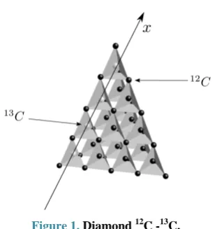
The above idea is represented in Figure 1, where the 13C atoms are place on the position of some 12C atoms. This replacement could be done using the same technics used to construct the diamond NV structure [23], or using ion implantation technics [24] and neutralization of 13C in the diamond [25]. It is assumed in this paper that this configuration can be built somehow.

Now, as one can see, the important interaction on this configuration is the spin-spin interaction between the nucleus of the 13C atoms. This interaction is well known [26] and is given by

(

1

)(

2

)

1 2

3 ,

4

o

U =µ ⋅ ⋅ − ⋅

π

m x m x m m

(2)

[image:2.595.96.252.77.241.2]

Figure 1. Diamond 12C -13C.

where the magnetic moment m_i,i=1, 2 of 13C’s is related with the nuclear spin as

,

i=γ i

m S (2)

being γ the proton gyromagnetic ratio

(

8

)

2.675 10 rad T s

γ ≈ × ⋅ . Without loosing the main idea, it will be assumed here that 13C magnetic moment is due to proton. The variable x indicates the separation vector between two 13C nucleus, which has magnitude

10

10 m

a= x  − . Aligning the chain of 13C nucleus along the x-axis of the reference system and assuming Ising interaction between 13C nucleus, this energy can be written as

1 2,

z z

J

U = S S

,

B (5)

where b, ϕ, and ω are the magnitude, the phase, and the frequency of the transverse rf-field. The z-component of the magnetic field has a gradient on the x-axis, determined by the difference on Larmore’s frequencies of the 13C’s nuclear magnetic moments,

0 _. B x x ω γ ∆ ∆  _{ =}  _∆  _∆

  (6)

The magnetic field at the location of the ith-13C atom is Bi

( )

t =B

(

x ti,

)

, and the interaction energy of the

magnetic moments of the 13C atoms with the magnetic field is

( )

1 , N i i i U t =

= −

∑

m B⋅ (7)

where N is the number of 13C atoms aligned along the x-axis. This energy can be written as

(

)

1

1 1

e e ,

2

N N

z i i

j j k k

j k

U ω S θS θS

−

− − +

= =

Ω

= −

∑

−

∑

+ (8)

where ω_j is the Larmore’s frequency of the ith-13C,

( )

0 ,

j B xj

ω =γ (9)

Ω is the Rabi’s frequency,

,

b

γ

Ω = (10)

j

S− and Sj

+

are the ascent and descent spin operators,

x y

j j j

S± =S iS , and θ has been defined as .

t

θ ω ϕ= + (11)

Let us consider first and second neighbor interactions among 13C nuclear spins, and assuming equidistant separation between any pair of spins, the Hamiltonian of the system is

(

)

1 1 1 1 2 2 1 1

e e ,

2

N N

z z z

j j j j

j k

N N

z z i i

l l j j

l j

J

H S S S

J

S S θS θS

ω − ₊

= = − − − + + = = = − + ′ Ω + − +

∑

  (12)

where J is the coupling constant of first neighbor 13C atoms, and J′ is the coupling constant of second neighbor 13C atoms which must be about one order of magnitude lower than J. One can write this Hamil- tonian as H =H0+W t

( )

, where H0 and W are

defined as

1 2

0 1 2

1 1 1

,

N N N

z z z z z

j j j j l l

j k l

J J

H ω S S S S S

− −

+ +

= = =

′

= −

∑

+

∑

+

∑

  (13)

and

( )

(

)

1

e e .

2

N

i i

j j

j

W t θS− −θS+

=

Ω

= −

∑

+ (14)

The operator H0 is diagonal on the basis

{

1

}

_0,1

k

N _ξ

ξ = ξ ξ ₌ of the Hilbert space of 2N dimensionality. Its eigenvalues defines the spectrum of the system,

( )

1 2 1 1 1 2 1 1 1 2 2 1 2

j k k

l l N N j j k N l J E J

ξ ξ ξ

ξ ξ ξ ω + + − ₊ = = − ₊ =  = − − + −  ′  + − _ 

∑

 (15)

Since J′ <Jω_j for j=1,,N, this spectrum is not degenerated with E000 as the energy of ground

state, and E_{11 1}_ as the energy of the most exited state. To calculate the spectrum, one has used the following action of z

j

S operator

( )

1 .

2

j

z j

(3)

The Schrödinger’s equation,

,

i H

t

∂ Ψ

= Ψ

∂

 (17)

is solved by proposing a solution of the form

( )

,

C_ξ t ξ

ξ

Ψ =

∑

(18)

which brings about the following system of first order differential equations on the interaction representation

( )

_{( )}

,

ei E E t ,

i a_δ a_ξ δ ξ W_{δ ξ} t

ξ −

=

∑

 

 (19)

where a_δ and W_{δ ξ}_, are defined as

( )

e iE t

aδ t =Cδ t − δ  (20)

and

( )

, .

Wδ ξ t = δ W t ξ (21)

This is very well known procedure to solve time dependent Schrödinger’s equation, and the solution of Equation (19) brings about he unitary evolution of the system (given the initial condition Ψo ).

Defining the evolution parameter τ through the change of variable t=ω τo

(

CCNOT quantum gate corresponds to the transition

)

(

)

2 1 1 f , 3 1 1 2f

ω =ω + ω =ω + (23)

where f measures the relative change of the frequencies of qubits. The separation of the 13C nucleus,

a, is parametrized as

10

10 m.

a= ⋅ξ − (24) For the CNOT quantum gate, one has the initial conditions C₀₀

( )

0 =C₀₁

( )

0 =C₁₁

( )

0 =0 and

( )

10 0 1

C = . The time is allowed to last a π-pulse

(

τ = π Ω

)

, and one takes the coupling constant as a fixed paramenter,

0.12, 1.

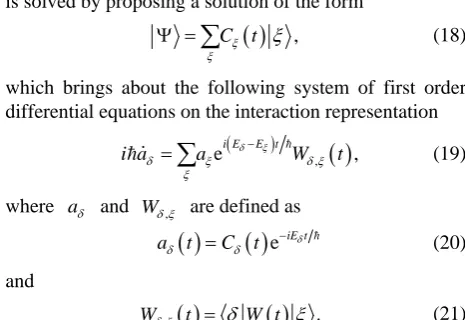
[image:3.595.54.287.139.299.2]

J= ξ = (25)

Figure 2shows the fidelity parameter,

2 ideal real ,

F = Ψ Ψ (26)

at the end of the π-pulse, as a function of the Rabi's frequency, where Ψreal is the state obtained with the

simulation, and Ψideal is the expected state

( )

11 .

The simulation was done for two different weak magnetic fields and for f =0.01 (1), f =0.05 (2),

0.1

f = (3), and f =0.2 (4). The oscillations seen on this picture are due to the low and high contribution of the non resonant states ( 00 and 01 ) to the dynamics of the system, which depends on Rabi’s frequency and they are explained by the 2πk-method [19]. As one can see from this picture , the CNOT gate is very well produced either with B01=0.1 T and f =0.2 or with

01 0.5 T

B = and f =0.05.

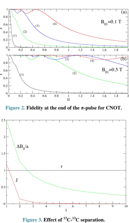
Figure 3 shows the gradient of magnetic field along the x-axis, the coupling constant J, and the fidelity F

of the CNOT quantum gate as a function of the two qubits separation (characterized by the parameter ξ, Equation (24)), having f =0.05. As one can see, the fidelity is not sensitive for relatively wide variation of ξ, meanwhile the gradient and coupling constant have the strong variation deduce from Equation (6) and Equation (4). Considering the separation of the two 13C atoms about the the length of the diamond unit cell, one can select ξ =3, corresponding to a coupling constant of

0.00445

J= , and a magnetic field gradient of

6

0 0.83 10 T m

B a

∆ ≈ × .

(4)

[image:4.595.60.287.71.463.2]

Figure 2. Fidelity at the end of the π-pulse for CNOT.

Figure 3. Effect of 13C-13C separation.

the longitudinal magnetic field), the coupling constant deduced from Equation (1) would be given by 2− J, with J given by Equation (4), and basically the results are the same as the presented here.

According to these results, one has now an idea of the value of the parameters for the design of a quantum computer with the 12C - 13C diamond quantum system: (a) Separation between 13C atoms is _a_{= ×}_{3 10}−10 _m

which can be aligned along the x-axis, (b) coupling constant is

(

)

0.00445 2 MHz

J= π , (c) longitudinal magnetic field

is B01=0.05 T , (d) gradient of this longitudinal

magnetic field along the x-axis is

6

0 0.83 10 T m

B a

∆ = × , and (e) magnitude of the rf-magnetic field on the plane x-y is b=0.00608 T (Rabi's frequency Ω =0.259 2 Mhz

(

π

)

).

For the CCNOT quantum gate, one has the initial conditions Ckji

( )

0 =0 for k= ≠j 1 and C110

( )

0 =1.

[image:4.595.310.537.84.247.2]

The time is allowed to last a π-pulse

(

τ = π Ω

)

. The coupling parameter J is taken as before, and second neighbor coupling parameter J′ =J 10.Figure 4 shows the fidelity parameter as a function of Rabi’s frequency for magnetic field intensities (1) B_o =0.01 T, (2)

Figure 4. Fidelity at the end of the π-pulse for CCNOT.

0.05 T

o

B = , (3) B_o =0.1 T, and (4) B_o =0.2 T, for

0.05

f = (a), and for f =0.1 (b). As one can see fro these plots, a good CCNOT quantum gate can be obtained by choosing f =0.1 (implying and encresing of the gradient of the magnetic field by a factor of two), and with the other parameters given as defined with the CNOT quantum gate.

Although the gradient of the magnetic field might be a concern, the magnitude of the longitudinal magnetic field is low enough to think that this gradient can be achieved. The scalability of the system is clear, the read out system could be based on single spin measurement technics [29], and studies on decoherence remains to be done on this system. This quantum computer resembles a solid state NMR system [30].

5. Conclusion and Discussion

(5)

of the 13C atom along the x-axis produces different coupling constant in the interaction, but according to

Figure 4, the fidelity of the CNOT quantum gate does not change, and one would expect the same result for quantum algorithms. The displacement of 13C atoms off x-axis changes the coupling constant and the interaction itself, which has to be studied. In addition, it still remains to study the decoherence on this system. Finally, one recalls that the carbon isotopesatoms 12C, 13C and 14C occur naturally on Earth with a percent of about 99%, 1% and 10−4%, 14C being a radioactive isotope with a half life of about 5730 years and havingspin zero. Therefore,

14

C is not an important composition at all in the diamond structure.

REFERENCES

[1] H.-P. Breuer and F. Petruccione, “The Theory of Open Quantum Systems,” Oxford University Press, Oxford, 2006.

[2] A. O. Caldeira and A. T. Legget, Physica A: Statistical Mechanics and its Applications, Vol. 121, 1983, pp. 587- 616. http://dx.doi.org/10.1016/0378-4371(83)90013-4

[3] W. G. Unruh and W. H. Zurek, Physical Review D, 1989, Vol. 40, pp. 1071-1094

http://dx.doi.org/10.1103/PhysRevD.40.1071

[4] B. L. Hu, J. P. Paz and Y. Zhang, Physical Review D, Vol. 45, 1992, pp. 2843-2861.

http://dx.doi.org/10.1103/PhysRevD.45.2843

[5] A. Venugopalan, Physical Review A, Vol. 56, 1997, pp. 4307-4310. http://dx.doi.org/10.1103/PhysRevA.56.4307

[6] H. D. Zeh, Foundations of Physics, Vol. 3, 1973, pp. 109- 116. http://dx.doi.org/10.1007/BF00708603

[7] J. P. Paz and W. H. Zurek, Proc. Les Houches, Vol. 111A, 1997, p. 409.

[8] G. Lindblad, Communications in Mathematical Physics, Vol. 48, 1976, pp. 119-130.

http://dx.doi.org/10.1007/BF01608499

[9] W. S. Warren, Science, Vol. 277, 1997, pp. 1688-1690. http://dx.doi.org/10.1126/science.277.5332.1688

[10] L. M. L. Vandersypen, M. Steffen, G. Breyta, C. S. Yan- noni, M. H. Sherwood and I. L. Chuang, Nature, Vol. 414, 2001, p. 883. http://dx.doi.org/10.1038/414883a

[11] M. H. Holzschelter, Los Alamos Science, Vol. 27, 2002, p. 264.

[12] C. Monroe and J. Kim, Science, 2013, Vol. 339, p. 1164. http://dx.doi.org/10.1126/science.1231298

[13] H. Walter, B. T. H. Varcoe, B. G. Englert and T. Becker,

Reports on Progress in Physics, Vol. 69, 2006, p. 1325. http://dx.doi.org/10.1088/0034-4885/69/5/R02

[14] D. Jaksch, J. I. Cirac, P. Zoller, S. L. Rolston, R. Côté and M. D. Lukin, Physical Review Letters, Vol. 85, 2000, pp. 2208-2211.

http://dx.doi.org/10.1103/PhysRevLett.85.2208

[15] K. C. Younge, B. Knuffman, S. E. Anderson and G. Rai- thel, Physical Review Letters, Vol. 104, 2010, Article ID: 173001.

http://dx.doi.org/10.1103/PhysRevLett.104.173001

[16] I. Chiorescu, Y. Nakamura, C. J. P. M. Harmans and J. E. Mooij, Science, Vol. 299, 2003, pp. 1869-1871. http://dx.doi.org/10.1126/science.1081045

[17] A. Yu. Kitaev, Annals of Physics, Vol. 303, 2003, pp. 2-30. http://dx.doi.org/10.1016/S0003-4916(02)00018-0

[18] L. Childress and R. Hanson, MRS Bulletin, Vol. 38, 2013, pp. 134-138. http://dx.doi.org/10.1557/mrs.2013.20

[19] G. P. Berman, D. I. Kamenev, D. D. Doolen, G. V. López and V. I. Tsifrinovich, Contemporary Mathematics, Vol. 305, 2002, p. 13.

http://dx.doi.org/10.1090/conm/305/05213

[20] G. V. López and L. Lara, Journal of Physics B: Atomic,

Molecular and Optical Physics, Vol. 39, 2006, p. 3897. http://dx.doi.org/10.1088/0953-4075/39/18/019

[21] G. V. López, T. Gorin and L. Lara, Journal of Physics B:

Atomic, Molecular and Optical Physics, Vol. 41, 2008, Article ID: 055504.

http://dx.doi.org/10.1088/0953-4075/41/5/055504 [22] G. V. López and P. López, Journal of Modern Physics,

Vol. 3, 2012, pp. 85-101.

http://dx.doi.org/10.4236/jmp.2012.31013

[23] K. Lakoubovskii and G. J. Adriaenssens, Journal of Physics: Condensed Matter, Vol. 13, 2001, p. 6015.

[24] R. W. Hamm and M. E. Hamm,“Industrial Acceleretors and Their Applications,” World Scientific, Singapore, 2012.

[25] M. A. Cazalilla, N. Lorente, R. D. Muño, J. P. Gauyacq, D. Teillet-Billy and P. M. Echenique, Physical Review B, Vol. 58, 1998, pp. 13991-14006.

http://dx.doi.org/10.1103/PhysRevB.58.13991

[26] J. D. Jackson, “Classical Electrodynamics,” 3rd Edition, Chapter 5.6, John Wiley and Sons, Inc., Hoboken, 1999.

[27] A. N. Kolmogorov and S. V. Fomin,“Introductory Real Analysis,” Dover Publications, Inc., Mineola, 1970.

[28] M. A. Nielsen and I. L. Chuang, “Quantum Computation and Quantum Information,” Cambridge University Press, Cambridge, 2000.

[29] D. Rugar, R. Budakian, H. J. Mamin and B. W. Chui,

111 e 011 e 101 e 011

2

i i i

ia = −Ω φ a + φ a + φ a (38)

)

ij t Ei Ej t

φ = ± + +ω ϕ − , where decimal i corres-