Consensus Control for a Kind of Dynamical Agents in Network

(1)

Published Online January 2016 in SciRes. http://www.scirp.org/journal/ijcns http://dx.doi.org/10.4236/ijcns.2016.91003

Consensus Control for a Kind of Dynamical

Agents in Network

Hongwang Yu

School of Science, Nanjing Audit and University, Nanjing, China

Received 27 November 2015; accepted 24 January 2016; published 27 January 2016

This work is licensed under the Creative Commons Attribution International License (CC BY). http://creativecommons.org/licenses/by/4.0/

Abstract

This paper discusses consensus control for a kind of dynamical agents in network. It is assumed that the agents distributed on a plane and their location coordinates are measured by remote sensor and transmitted to its neighbors. By designing the linear distributed control protocol, it is shown that the group of agents will achieves consensus. The simulations are given to show the ef-fectiveness of our theoretical result.

Keywords

Distributed Control, Graph Laplacian, Dynamical Agents

1. Introduction

Distributed coordination of network of dynamic agents has attracted a great attention in recent years. Modeling and exploring these coordinated dynamic agents have become an important issue in physics, biophysics, systems biology, applied mathematics, mechanics, computer science and control theory [1]-[11]. How and when coordi-nated dynamic agents achieve aggregation is one of the interesting topics in the research area. Such problem may also be described as a consensus control problem.

To describe the collective behavior of agents in a large scale network, the agent in the network usually is modeled by a very simple mathematical model, which is an approximation of real objects. Saber and Murray [3] [4] proposed a systematical framework of consensus problems in networks of dynamic agents. In their work the dynamics of the agent is modelled by a simple scalar continuous-time integrator x=u, the convergence analy-sis is provided in different types of the network topologies. Following the work of [3] [4], Guangming Xie [10]

(2)

structure of the graph, the dynamical agents will eventually achieve aggregation, i.e. all agents will gradually move into a fixed position, meanwhile their velocities converge to zero.

In our work a similar problem is studied under the condition that the agents move in a plane. The agents may represent the vehicles or mobile robots spread over a wild area and they communicate by means of some remote sensors with certain error. When the agents are moving in a plane, the collective behavior conditions will depend on the communicated error and the algebraic characterization of the communicated network topology, as well as the dynamical behavior of agents.

This paper is organized as follows. In Section 2, we recall some properties on graph theory and give the prob-lem formulation. In Section 3 the main results of this paper are given and some simulation results are presented in Section 4. Final section is a conclusion.

2. Preliminaries

Consider a network of dynamical agents defined by a graph G =

(

V E A, ,

)

. The node set V consists of dynamical agents p ii; ∈M . The dynamics of pi for i∈M is described as follows.

Let x_i=

(

x x_i₁, _i₂

)

τ∈R2 be the coordinate of dynamical agent p_i in 2

R , then the dynamical equation of agent p_i is

i i i i i i

i i

i

x v

m v kv u

x

y F

v =

= +

  =    



 (1)

where xi

(

x xi1, i2

)

τ

= indicates the location of agent p_i in the plane, vi

(

v vi1, i2

)

τ

= represents the velocity of

the i-th agent and m_i is its mass and 11 12 21 22

k k

k

k k

 

=  

  is a dynamical feedback matrix of the agent. F is an observation matrix of the agent by some remote sensor.

In what follows we simply assume that mi=1 for all i∈M and pi =xi. Let F=

[

C 0

]

which means that the location information of the i-th agent is only measured by some remote sensor and is transmitted to its

neighbors through the network. The matrix C is assumed to be an orthogonal matrix in the form 1 1

C δ

δ

 

= _₋ _.

The parameter

δ

will indicates that the network transmitted error or the coordinates used for sensor could be different from that of the agents.

For the dynamic agent (1) in network we have following assumption.

Assumption 2.1 The dynamics (1) is Lyapunov stable when it disconnected with its neighbors, meaning that the dynamical agent as an autonomous will gradually stop by moving a finite distance for any non-zero initial velocity vi

( )

0 .

The collective behavior of dynamical agents in network can be described by

( )

(

( ) ( )

( )

)

2

1 2

: , , , M M

x t = xτ t xτ t  xτ t τ∈R ; t≥0. We denote the initial locations and the initial velocities of the

system as x

( )

0 =

(

x₁τ

( )

0 ,,xτ_M

( )

0

)

τ, v

( )

0 =

(

v₁τ

( ) ( )

0 ,v₂τ 0 ,,vτ_M

( )

0

)

τ respectively.

In this work, we discuss the collective behavior of the dynamical agents under a decentralized control law in the form that

(

1, 2, , li

)

i i j j j

u =K y y  y (2)

where indexes

{

₁, ₂, ,

}

i

l

j j  j ⊂M .

We claim that a group of dynamical agents associated with G =

(

V E A, ,

)

asymptotically achieve the collective behavior under control protocol (2). That is to say, for any initial conditions of the agents xi

( )

0 ∈R2,

( )

2

0 i

(3)

( )

*

( )

lim _i , lim _i 0

t→∞x t =x t→∞v t = (3) In our work, let (2) be

(

)

j i

i ij j i x N

u a y y

∈

=

∑

− (4)

where N_i is the set of neighbors of agent p_i.

Remark 1: If we choose k₁₁=k₂₂=k k, ₁₂=k₂₁=0 and

δ

=0, then the two-dimension agent systems (1)

with the control protocol (4) can be decoupled into two identical linear systems of the form

is is x =v

(

)

j i

i is is ij js is p N

m v kv a x x

∈

= +

∑

−



for s=1, 2. i.e. dim xi=1, and it was discussed in [12].

3. Collective Behaviors of Dynamical Agents

Consider a group of dynamical agents in network associated with a graph G =

(

V E A, ,

)

. The node set V

consists of dynamic p ii; ∈M . The dynamical pi for each i∈M is described by linear dynamical equation (1) satisfying Assumption 2.1. Under control protocol (4) the dynamical equation of agent p_i is written by

(

)

j i

i i

i i ij j i

p N

x v

v kv a y y

∈ =

= +

∑

−



 (5)

Denote i

(

x vi, i

)

(

xi₁,xi₂,v vi₁, i₂

)

, i M

τ τ

ξ

= = ∈ , then (5) is written in

(

)

j i

i i ij j i

p N

A B a

ξ ξ ξ ξ

∈

= +

∑

−

 (6)

where 2 2 2 2 2 2 2

2 2 2 2

0 0 0

, .

0 0

I

A B

k C

× × ×

× ×

   

=_ _ =_ _

   

Let

(

1, 2, , M

)

τ τ τ τ

ξ

=

ξ ξ

_

ξ

, then the dynamic network is of the following form.

ξ= Ωξ (7)

where

M

I A L B

Ω = ⊗ − ⊗ (8)

and L is the aforementioned Laplacian associated with the graph G .

The collective behavior problem of dynamical agents can be described in

χ

-consensus asymptotical con-sensus stability ([3]). Let 4 2

:R M R

χ → be a map, for

( )

(

( ) ( ) ( ) ( )

( )

)

4

1 1 2 2

0 : 0 , 0 , 0 , 0 , , 0 , 0 M

M M

x v x v x v τ R

ξ =  ∈ ,

χ ξ

:

( )

0 x

( )

∈R2 . The group of dynamical agents is called

χ

-consensus asymptotically stable under control protocol (4) if let

χ ξ

(

( )

0

)

=x* for a given

( )

0

ξ , then for each agent in network its state variables meets the properties of (3).

As dynamics (7) is a standard linear time-invariant dynamical system, its trajectory can be described by

( )

t exp

( ) ( )

t 0

ξ = Ω ξ (9)

The consensus asymptotical stability implies that the matrix exp

( )

Ωt converges to a constant matrix, thus we will explore some properties of the matrix Ω.

Lemma 3.1 The matrix Ω has two eigenvectors associated with zero eigenvalue. Let v vr, l be the right

and left eigenvectors (denoted by matrices) of matrix Ω associated with zero eigenvalue, respectively. Then

1

2 2 2

1 1

, 0

r M l M

k k

v v

I

M M

τ τ

−

×

   

= ⊗_ _ = ⊗_ _

−

   

(4)

and v v_{l r} =I₂, where 1_M =

(

1,1,,1

)

τ∈RM

Proof: It is well known that the graph G =

(

V E A, ,

)

is connected if and only if its Laplacian satisfies that rank L

( )

=M −1. Moreover, 1_M =

(

1,1,,1

)

τ∈RM is an eigenvector of L associated with eigenvalue

0

λ

= , i.e., L⋅1M = ⋅0 1M. Then, there is only one zero eigenvalue of L, all the other ones are positive and real. By the definition of (8) one has

(

)

1 1

2 2 2 2

2 2

4 2 1

1 1

0 0

0

1 1

0 0

M M M

M M

k k

I A L B

M M

Pk

M M

− −

× ×

×

× −

   

Ω ⋅ ⊗_ _= ⊗ − ⊗ ⋅ ⊗_ _

   

 

= ⊗ − _{⊗ } _

 

1 1

1

Thus,

1

2 2 1

0

r M

k v

M

−

×

 

= _{⊗ } _

 

1 represented two right-eigenvectors of Ω associated with zero-eigenvalue.

Similarly, it is easy to check

[

2

]

1

l M

v k I

M τ

= 1 ⊗ − represents two left-eigenvectors of Ω and v vl r =I₂. 

The following Lemma is key to our work.

Lemma 3.2 If the control gain k in dynamical agent (1) satisfies Assumption 2.1, and

δ

in the C of (4) sa-tisfies

1 2,

δ < <δ δ (11)

with

(

)

(

)

1 2 2 , 2 2 2

2 2

abc abc

a b a b

δ δ

λ λ

− ∆ + ∆

= =

+ + (12)

where a=k₂₁−k₁₂, b= −k₁₁−k₂₂, c=k k_{11 22}−k k_{12 21}, ∆ =

(

abc

)

2+4λ

(

a2+b2

)

b c2 and λ λ= _M denotes the biggest eigenvalue of matrix L, then it is hold that

( )

lim exp _{r l}

t→∞ Ω =t v v (13) Proof: Denote the eigenvalues of L by 0=λ₁<λ₂≤λ₃≤≤λM, and let Λ be the Jordan form associated with L, there exists an orthogonal matrix W such that W LW diag

{

₁, ₂, , M

}

τ _{= Λ =} _{λ λ} _ _λ _.

One can verify the following formulae.

(

)

(

)

(

)

(

)(

)

{

}

4 4 4 4

1 2

diag , , ,

M

W I W I W I I A L B W I

I A B

A B A B A B

τ τ

λ λ λ

⊗ ⋅ Ω ⋅ ⊗ = ⊗ ⊗ − ⊗ ⊗

= ⊗ − Λ ⊗

= − −  −

The dynamical behavior of the network (7) is characterized by the eigenvalues of A−λ_iB for

{

1, 2, ,

}

i∈  M .

First we discuss the block with λ =₁ 0. By Assumption 2.1, one has k₁₁+k₂₂ <0,k k_{12 21}<k k_{11 22} and

(

1

)

2

rank A−λB =rank A= , its four characteristic eigenvalues must satisfy s₁=s₂ =0 , Re s

( )

₃ <0 ,

( )

4 0.

Re s < .

For λ >i 0, one has

2 2 2 0 i

i I

A B

C k

λ

λ ×

 

− _{= } _

−

 . As rank C

( )

=2, rank A

(

−λiB

)

=4. Therefore, Ω has on-ly two zero eigenvalues.

Consider the characteristic polynomial of A−λiB i; ∈M

( )

(

)

4 3 2

1 2 3 4

11 12

21 22

0 1 0

0 0 1

=

i

A B i

i i

s s

s det sI A B s a s a s a s a

s k k

k s k

λ

π

λ

δλ

λ

−

= − − = + + + +

− −

(5)

where

(

)

(

)

(

)

1 11 22 2 11 22 12 21

3 21 12 11 22

2 2

4

, 2 ,

,

1

i

i i

i

a k k a k k k k

a k k k k

a λ δλ λ λ δ = − − = − + = − − + = + (14)

Construct the Routh array of

( )

i AλB s π − 4 2 4 3 1 3 2 1 2 1 1 0 1 1 0 0 0

s a a

s b b

s c

s d

with

(

)

2 2

1 2 3 1 3 1 2 1 2 3 3 1 4

1 2 1 4 1

1 1 1 1

, i 1 , .

a a a b a a b a a a a a a

b b d a c

a λ δ b a b

− − − −

= = = = − = = By the Routh-Hurwith

criterion, for stability it is necessary that a₁>0,b₁>0,c₁ >0,d₁>0. Therefore, the dynamical network is stable if the following inequalities hold

1

4

1 2 3

2 2

1 2 3 3 1 4

0 0 0 0 a a

a a a

a a a a a a

>   > 

 ₋ _> 

 ₋ ₋ _>



(15)

By (14) one has

(

) (

)

(

) (

)

(

) (

)

(

)

1 2 3 11 22 11 22 12 21 21 12 11 22

11 22 11 22 12 21 21 12 11 22

2 i i

i

a a a k k k k k k k k k k

k k k k k k k k k k

λ λ δ

λ δ

− = − + ⋅ − + − _ − − + _

= − + ⋅ − − _ − + + _ (16)

and

(

) (

)

(

)

{

}

(

) (

)

(

)

(

) (

)

(

) (

)

{

}

(

) (

)

2 2

1 2 3 3 1 4 11 22 11 22 12 21 21 12 11 22

2 2 2

21 12 11 22 11 22

11 22 11 22 12 21 21 12 11 22

2 2

11 22 21 12

1 i

i i

i

a a a a a a k k k k k k k k k k

k k k k k k

k k k k k k k k k k

k k k k

λ δ

λ δ λ δ

δ λ λ δ − − = − + ⋅ − + _ − + + _ × _ − − + _− + + = − + ⋅ − ⋅_ − − + _   + _ + + − _ (17)

The inequalities (15) can be rewritten as the following form by using the conditions of Lemma 3.2 and the Equations (16)-(17).

(

)

(

)

2 2 2 2

0

b c a

b c abc a b

λ λ δ

δ λ δ

 + − >

 

+ − + >

 (18)

We can further show that the second inequality in above implies the first one. Obviously, it is true when 0

a= . If a>0, one gets

(

)

1 2 b c a λ δ λ

δ δ δ

+ 

<    < < 

where δ =i,i 1, 2 are defined in (12).

(6)

(

)

(

)

(

)

(

)

(

)

(

)

(

)

(

)

2 2 2 2 2 2 2 2

2 2 2 2

2 2 2 2 2 2 2 2

2

2 2 2 4 2 2 2 2 2 2 2

4 4

2 2

2 2 4

4 4 8 4 0

abc b a c a b c ac a c a b c

b c c

a a b a a b

a b a c b c a a c a b c

a b b c a b b c a b c

λ λ λ λ λ λ λ λ λ λ + + + + + + + +

> ⇔ >

+ +

⇔ + + + > + +

⇔ + + + + + >

The last inequality obviously holds. Therefore, the solution of (18) leads δ₁< <δ δ₂.

If a<0, one can obtain b

(

c

)

a

λ

δ

λ

+

> and δ₁< <δ δ₂. So we can get that 1

(

)

b c a

λ

δ

λ

+

> with a similar

computing process. It shows that δ₁< <δ δ₂ is the solution set of the inequalities (15) for any a. Therefore, A−λiB; 2≤ ≤i M are Hurwitz.

By :

(

1, 2, , 4 1, 4

)

4 4 M M

M M R

θ θ θ θ ×

−

Θ =  ∈ one denotes right-eigenvectors of Ω associated with eigenvalues

1, 2, , 2M

γ γ  γ , respectively. Thus,

2

1

2

1

0 0 0 0 0

0 0 0 0

M M J J J J J −        

ΩΘ = Θ = Θ

                   

where J₁ denote the Jordan form of two order associated with the eigenvalues γ₁, and γ₂. J_i denote the Jordan form of four order associated with the eigenvalues γ₄_i₋₃, γ₄_i₋₂, γ_{4 1}_i₋ and γ₄_i for all i=2, 3,,M .

Let 1

(

)

4 4

1 2 4 1 4

: , , , , M M

M M R

τ τ τ τ τ

θ θ θ θ

− ×

−

Θ = Θ =   _   ∈ , where θi;i∈4M are 4M row left-eigenvectors of Ω,

correspondingly.

2

1

2

1

0 0 0 0 0

0 0 0 0

M M J J J J J −        

ΘΩ = Θ = Θ

                      

As 0>Re

( )

γ₃ ≥Re

( )

γ₄ ≥≥Re

(

γ₄_M−₁

)

≥Re

(

γ₄_M

)

, one has

( )

( ) ( ) ( )

2 2 4 2

4 2 2 4 2 4 2 0 lim e 0 0 M Jt t

M M M

I _× ₋

→∞ − × − × −   =       and

( )

( ) ( ) ( ) ( )

2 2 4 2

4 2 2 4 2 4 2 0 lim exp

0 0

M

t

M M M

I

t × −

→∞

− × − × −

 

Ω = Θ Θ

 

 



Let v_l =

(

θ θ₁ ₂

)

and 1 2 r v θ θ   =  _{ }   

 , one has

( )

lim exp _{r l}. t→∞ Ω =t v v Due to the fact that 1

4M4M I

−

×

Θ ⋅ Θ = Θ ⋅ Θ = , v_r and v_l satisfy the property v v_{l r} =I₂. 

(7)

the collective behavior of the dynamic agents.

Proof: As ξ

( )

t =exp

( ) ( )

Ωt ξ 0 and lim_t→∞exp

( )

Ω =t v v_{r l}, it follows that

( )

( ) ( )

( )

[

]

( )

1

1 1

2 2

2 2 2 2 2 2

lim lim exp 0 0

0 0

1 1

0

0 0 0

0 0 r l

t t

M M M M

M

t t v v

x v

k I k

k I

M M

x v

τ τ

ξ ξ ξ

ξ →∞ →∞

− −

× × ×

= Ω =

 

 

   −  _ _

= ⊗_ _⋅ ⊗ − = ⊗_ _{ }⋅



   

 

 



1 1 1 1

Therefore,

( )

1

( )

1 1

lim 0 0

M

i j j

t

j

x t x k v

M

−

→∞ ₌

 _ _

= _ _ − __



∑

 (19)

and it is obvious that

( )

{

}

lim _i 0, 1, 2, , t→∞v t = i∈  M

(20)

This implies the protocol (5) globally asymptotically achieve aggregation. 

Corollary 3.1 If the control gain k satisfies k₁₂=k₂₁ and λδ <2

(

k k_{11 22}−k k_{12 21}

)

, then the control protocol

(4) globally and asymptotically achieves the collective behavior of the dynamic agents.

Under Assumption 2.1 one has k k_{12 21}<k k_{11 22}. Thus, by carefully examining (12) one finds that c>0 and it further implies that δ <₁ 0 and δ >₂ 0 in (11). Thus we have the following.

Corollary 3.2 The dynamical agents achieve collective behavior if δ 1 in control protocol (4). Again, the

χ

-map is defined by (19) and (20).

4. Simulations

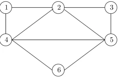
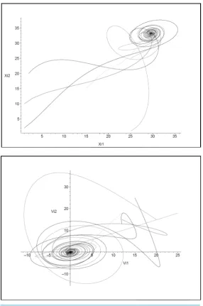
[image:7.595.84.539.115.325.2] [image:7.595.216.415.570.705.2]

We study some examples to show that our results are effective. The network of dynamic agents is described in

Figure 1.

We can obtain the Laplacian matrix L of the graph G of Figure 1 and its eigenvalues are λ =₁ 0,

(

)

2 3

1

7 13 2

λ =λ = − , λ =₄ 4, ₅ ₆ 1

(

7 13

)

2

λ =λ = + .

We consider that the dynamic agent (1) in the network has 1 0.1 0.2 1 k= − _

−

  and observation matrix 1 0.3

0.3 1

C=  _

−

 . Thus, it is Lyapunov stable and satisfies Assumption 2.1. One can get a=0.1, b=2,

(8)

0.98

c= , ∆ =16.5699, and the

δ

=0.3 belongs to the range of parameters i.e.

1 0.467617 0.478812 2

δ = − < <δ =δ .

When a control protocol (4) is applied into the agents in network, the collective behavior of dynamic agents takes place according to our result.

Figure 2 gives simulation results of the collective behavior of the agents with initial conditions

( )

11 0 12 0 15

x =x = , x₂₁

( )

0 =x₂₂

( )

0 =25, x₃₁

( )

0 =2, x₃₂

( )

0 =20, x₄₁

( )

0 =1, x₄₂

( )

0 =10, x₅₁

( )

0 =1,

( )

52 0 2

x = , x₆₁

( )

0 =25, x₆₂

( )

0 =1, and the initial velocities v₁₁

( )

0 =12, v₁₂

( )

0 =18, v₂₁

( )

0 =25,

( )

22 0 18

v = , v₃₁

( )

0 =15, v₃₂

( )

0 =25, v₄₁

( )

0 =12, v₄₂

( )

0 =15, v₅₁

( )

0 =12, v₅₂

( )

0 =13, v₆₁

( )

0 =20,

( )

62 0 15

v = .

It is found that when the agents approach to * 29.6 33.1 x =  _

 , the speeds of agents tend to zero.

5. Conclusion

[image:8.595.171.458.274.706.2]

We discuss the consensus control of dynamical agents in network which associated with a graph G . When the

(9)

agents are moving in a plane, the aggregation of the dynamical agents are depended on not only the communi-cated error, but also the algebraic characterization of the communicommuni-cated network graph and the dynamical prop-erties of agents.

Acknowledgements

This work was supported by the Natural Science Foundation of Jiangsu Higher Education Institutions of China (Grant no. 13KJB110015).

References

[1] Fax, A. and Murray, R.M. (2004) Information Flow and Cooperative Control of Vehicle Formations. IEEE Transac-tions on Automatic Control, 49, 1465-1476. http://dx.doi.org/10.1109/TAC.2004.834433

[2] Toner J. and Tu, Y. (1998) Flochs, Herds, and Schools: A Quantitative Theory of Flocking. Physical Review E, 58, 4828-4858. http://dx.doi.org/10.1103/PhysRevE.58.4828

[3] Saber, R.O. and Murray, R.M. (2003) Consensus Protocols for Networks of Dynamic Agents. Proceedings of the American Control Conference, 2, 951-956. http://dx.doi.org/10.1109/acc.2003.1239709

[4] Saber, R.O. and Murray, R.M. (2004) Consensus Problems in Networks of Agents with Switching Topology and Time-Delays. IEEE Transactions on Automatic Control, 49, 1520-1533. http://dx.doi.org/10.1109/TAC.2004.834113 [5] Liu, Y. and Passino, K.M. (2003) Stability Analysis of One-Dimensional Asynchronous Swarms. IEEE Transactions

on Automatic Control, 48, 1848-1854. http://dx.doi.org/10.1109/TAC.2003.817942

[6] Liu, Y. and Passino, K.M. (2003) Stability Analysis of M-Dimensional Asynchronous Swarms with a Fixed Commu-nication Topology. IEEE Transactions on Automatic Control, 48, 76-95. http://dx.doi.org/10.1109/TAC.2002.806657 [7] Gazi, V. and Passion, K.M. (2004) Stability Analysis of Social Foraging Swarms. IEEE Transactions on Systems, Man,

and Cybernetics, Part B, 34, 539-557.

[8] Liu, Y. and Passino, K.M. (2004) Stable Social Foraging Swarms in a Noisy Environment. IEEE Transactions on Au-tomatic Control, 49, 30-44. http://dx.doi.org/10.1109/TAC.2003.821416

[9] Savkin, A.V. (2004) Coordinate Collective Motion of Groups of Autonomous Mobile Robots: Analysis of Vicsek’s Model. IEEE Transactions on Automatic Control, 49, 981-983. http://dx.doi.org/10.1109/TAC.2004.829621

[10] Xie, G.M. and Wang, L. (2006) Consensus Control for a Class of Networks of Dynamic Agents. International Journal of Robust and Nonlinear Control, 17, 941-959.

[11] Algebraic, B.N. (1994) Graph Theory. Cambridge University Press, Cambridge, UK.