Analysis of the CNV waveform in the time and frequency domains

Analysis of the CNV waveform in the time and frequency

domains.

COELHO, Michael.

Available from Sheffield Hallam University Research Archive (SHURA) at:

http://shura.shu.ac.uk/19489/

This document is the author deposited version. You are advised to consult the

publisher's version if you wish to cite from it.

Published version

COELHO, Michael. (1988). Analysis of the CNV waveform in the time and frequency

domains. Masters, Sheffield Hallam University (United Kingdom)..

Copyright and re-use policy

See

http://shura.shu.ac.uk/information.html

SHEFFIELD LJi * POLYTECHNIC LIBRARY

>R£TND S.W^S*. £*i i ts k % tl/MP S T 1

100225473

1 7 0 *

Sheffield City Polytechnic Library

ProQuest Number: 10694370

All rights reserved INFORMATION TO ALL USERS

The quality of this reproduction is dependent upon the quality of the copy submitted. In the unlikely event that the author did not send a com plete manuscript and there are missing pages, these will be noted. Also, if material had to be removed,

a note will indicate the deletion.

uest

ProQuest 10694370

Published by ProQuest LLC(2017). Copyright of the Dissertation is held by the Author.

All rights reserved.

This work is protected against unauthorized copying under Title 17, United States C ode Microform Edition © ProQuest LLC.

ProQuest LLC.

789 East Eisenhower Parkway P.O. Box 1346

ANALYSIS OF THE CNV WAVEFORM IN THE TIME AND FREQUENCY

DOMAINS

by

MICHAEL COELHO

A thesis submitted to the Council for National Academic

Awards in partial fulfillment of the requirements for the

degree of Master of Philosophy

Sponsoring Establishment : Department of Electrical and

Electron!c Engineering, Sheffield City Polytechnic

Collaborating Establishments : Department of Neurological Sciences, Freedom Fields Hospital, Plymouth

I

(

ANALYSIS OF THE CNV WAVEFORM IN THE TIME AND FREQUENCY DOMAINS

M. COELHO ABSTRACT

The Contingent Negative Variation (CNV) response of the

Electroencephalogram (EEC) is often obscured by the

background EEC and/or ocular artefacts (OAs). These

necessitate the application of a variety of signal

processing techniques to reduce the influence of such phenomena on the measured signal. The methods discussed in this thesis are: ocular artefact removal (OAR) in the time domain and the use of data tapering and Fourier Transforms to give frequency domain amplitude and phase spectra.

Two OAR methods were compared: a non-recursive method using ordinary least squares parameter estimation developed by Nichols and a recursive least squares technique developed by Ifeachor. Recursive OAR was observed to distort the CNV response. This was discovered to be due to omission of the response from the algorithm being used, an omission ocurring in both techniques. To correct this the inclusion of a

model of the response in the algorithm was proposed. A

number of data sets were devised in order to investigate this effect and the successfulness of including the response model. It was shown that response modelling gave more

efficient OAR and reduced response distortion. Similar

investigations were performed on recorded response data which showed that modelling was essential for recursive OAR but that non-recursive OAR was relatively insensitive to the inclusion or omission of response modelling.

The use of data tapering was included in order to help improve the spectral analysis of short epochs of EEG data. A comparison of statistical properties of the harmonics of

the amplitude and phase spectra of the CNVs of normal,

ACKNOWLEDGEMENTS

Any such work owes much to others for their help and support.

First I must thank my supervisors Barrie Jervis and Elaine Allen for their advice and interest in this project. I must also thank Barrie Jervis for his critical comments on this thesis. Thanks also go to Geoff Morgan for discussions on the use of the least squares method and also for allowing me to use his predictive statistical diagnosis programmes. Thanks are also due to Martin Nichols and Emmanuel Ifeachor for their helpful comments on running their software on a different machine. In this respect I would also like to

thank the staff of the Computer Service sections of

Sheffield City and Plymouth Polytechnics: and the University of Sheffield. I would also like to express my gratitude to the staff of Sheffield City Polytechnic Library for their help in procuring all the material I studied from outside Sheffield.

For financial assistance I must thank Barry Plumb for arranging a Research Assistantship and the IEE for a postgraduate scholarship.

Finally I want to thank Detelina for all her encouragement and help.

COURSES AND SEMINARS ATTENDED

In accordance with regulations 3.8 and 3.9 I have attended and participated in the following:

Final year honours degree course in Signal Processing.

Jan 1985 and Oct-Dec 1985 EEG Society, Scientific Meeting, Birmingham.

CONTENTS

ABSTRACT ii

ACKNOWLEDGEMENTS i i i

1 INTRODUCTION 1

1.1 THE ELECTROENCEPHALOGRAM AND THE CONTINGENT

NEGATIVE VARIATION AND AUDITORY EVOKED

POTENTIAL RESPONSES 2

1.1.1 ORIGINS OF THE ELECTROENCEPHALOGRAM 2

1.1.2 DESCRIPTION OF THE ELECTROENCEPHALOGRAM 2

1.1.3 THE CONTINGENT NEGATIVE VARIATION 3

1.1.4 THE AUDITORY EVOKED POTENTIAL 4

1.1.5 OCULAR ARTEFACTS 4

1.2 TIME AND FREQUENCY DOMAIN METHODS OF

PROCESSING AND ANALYSING THE CONTINGENT

NEGATIVE VARIATION 5

1.2.1 OCULAR ARTEFACT REMOVAL 5

1.2.2 SPECTRAL ANALYSIS 7

1.2.3 STATISTICAL METHODS 7

1.2.4 THE APPLICATION OF THE CONTINGENT NEGATIVE

VARIATION TO HUNTINGTONS'S CHOREA FOR

DIAGNOSTIC PURPOSES 8

1.3 EXPERIMENTAL DATA RECORDINGS 8

1.4 GOALS AND AIMS OF THESIS 9

1.5 OVERVIEW OF THESIS 10

REFERENCES 11

2 OCULAR ARTEFACT REMOVAL 15

2.2.1 THE LEAST SQUARES METHOD OF PARAMETER

ESTIMATION 17

2.2.2 NON-RECURSIVE OCULAR ARTEFACT REMOVAL 18

2.2.3 RECURSIVE OCULAR ARTEFACT REMOVAL 19

2.3 OCULAR ARTEFACT REMOVAL WITH A RESPONSE

PRESENT 20

2.3.1 ERRONEOUS PARAMETER ESTIMATION DUE TO

PRESENCE OF NON-RANDOM RESPONSE 20

2.3.2 RESPONSE MODELLING IN THE APPLICATION OF

OCULAR ARTEFACT REMOVAL 24

2.4 THE EFFECT OF D.C. LEVEL REMOVAL 27

2.5 TEST DATA 29

2.5.1 DESCRIPTION OF TEST DATA 29

2.5.1.1 OA AND A SEPARATE RESPONSE 30

2.5.1.2 SEPARATE OA AND A RESPONSE HAVING AN

ADDITIONAL OA 40

2.5.1.3 CONTAMINATION OF THE EOG BY THE RESPONSE 47

2.5.1.4 REALISITIC TEST DATA 56

2.6 RESULTS USING REAL DATA 71

2.6.1 CNV RESPONSES 71

2.6.2 AEP RESPONSES 77

2.7 DISCUSSION 84

REFERENCES 86

3 FREQUENCY DOMAIN METHODS 89

3.1 CHAPTER OUTLINE 89

3.2 THE FOURIER TRANSFORM AND ENERGY SPECTRUM 90

3.2.1 BACKGROUND 90

3.2.3 THE USE OF THE SPECTRA I N : SIGNAL

PROCESSING 93

-v-3.2.2 ENERGY SPECTRUM 93

3.3 FURTHER SIGNAL PROCESSING TOPICS 95

3.3.1 SAMPLING AND ALIASING 95

3.3.2 PICKET FENCE (SCALLOPING) EFFECT 97

3.3.3 LIMITATIONS DUE TO DATA DURATION 98

3.4 THE USE OF DATA WINDOWS 99

3.4.1 SPECTRAL LEAKAGE AND DATA WINDOWS 99

3.4.2 THE TUKEY WINDOW ' 108

3.4.3 THE KAISER-BESSEL WINDOW 106

3.4.4 PROBLEMS WITH WINDOWING 107

3.5 INVESTIGATION OF SIGNAL PROCESSING CONCEPTS 112

3.5.1 TEST DATA 113

3.5.1.1 DESCRIPTION OF THE TEST DATA 113

3.5.1.2 APPLICATION AND RESULTS 113

3.5.1.3 DISCUSSION OF TEST DATA RESULTS 124

3.5.2 REAL DATA 125

3.5.2.1 DESCRIPTION OF DATA 125

3.5.2.2 RESULTS 125

3.5.2.3 DISCUSSION OF REAL DATA RESULTS 128

3.6 CONCLUDING REMARKS 128

REFERENCES 129

4 STATISTICAL METHODS 132

4.1 CHAPTER OUTLINE * 132

4.2 STATISTICAL TESTS 132

4.2.1 NEAREST AND FURTHEST MEAN AMPLITUDE TEST 133

4.2.2 PRE- AND POST- STIMULUS MEAN AMPLITUDE

4.3 DISCRIMINANT ANALYSIS 135

4.4 PREDICTIVE! STATISTICAL DIAGNOSIS 138

4.5 IMPLEMENTATION OF STATISTICAL METHODS 141

4.6 INTERPRETATION OF RESULTS OF DISCRIMINANT

ANALYSIS AND PREDICTIVE STATISTICAL

DIAGNOSIS 147

4.6.1 DISCRIMINANT ANAYLYSIS RESULTS 147

4.6.2 PREDICTIVE! STATISTICAL DIAGNOSIS RESULTS 148

REFERENCES 149

5 RESULTS OF PREDICTIVE'; STATISTICAL

DIAGNOSIS AND DISCRIMINANT ANALYSIS 152

5.1 CHAPTER OUTLINE 152

5.2 RESULTS 153

5.2.1 INTERMEDIATE RESULTS IN IMPLEMENTING

PREDICTIVE STATISTICAL DIAGNOSIS AND

DISCRIMINANT ANALYSIS 153

5.2.2 DIAGNOSTIC RESULTS OF THE LOGIC ALGORITHM 154

5.2.3 RESULTS OF APPLICATION OF PREDICTIVE

STATISTICAL DIAGNOSIS 155

5.2.3.1 PREDICTIVE STATISTICAL DIAGNOSIS AND THE

FULL DATA SET 15?

5.2.3.2 PREDICTIVE STATISTICAL DIAGNOSIS AND THE

OUTLIERS-REMOVED DATA SET 160

5.2.4 RESULTS OF APPLICATION OF DISCRIMINANT

ANALYSIS 164

5.2.4.1 DISCRIMINANT ANALYSIS AND THE FULL DATA SET 165

5.2.4.2 DISCRIMINANT ANALYSIS AND THE

OUTLIERS-REMOVED DATA SET 167

5.3 DISCUSSION 169

-vii-5.4 CONCLUSIONS 172

REFERENCES 173

6 CONCLUSIONS 175

6.1 RESULTS AND PROCESSING METHODS 175

6.2 SUGGESTIONS FOR FUTURE INVESTIGATION 177

6.3 CONCLUDING REMARKS 178

APPENDICES A1

APPENDIX A1 DERIVATION OF THE ESTIMATES FOR THE 8 .s _j A1

APPENDIX A2 PROGRAM UNIT LISTINGS AND DESCRIPTIONS A4

A 2 . 1 CALLING SEQUENCES A4

A2.2 PROGRAM UNIT DETAILS A6

1 INTRODUCTION

The following points are discussed,in this chapter :

the origins of this thesis; the data processing methods to

be applied; and the goals and aims of the thesis.

Section 1.1 is a desription of the thesis origins and a

brief overview of the relevant areas in the field of EEG

work, an outline of the Contingent Negative Variation (CNV)

and Auditory Evoked Potential (AEP) responses of the human

EEG, and Ocular Artefacts (OAs). The time and frequency

domain methods to be applied are given in Section 1.2.

These comprise Ocular Artefact Removal (OAR) in the time

domain, signal processing methods of windowing (time domain)

of data prior to transformation to the frequency domain

phase and energy spectra.

The statistical methods applied

1.1 THE ELECTROENCEPHALOGRAM AND THE CONTINGENT NEGATIVE VARIATION AND AUDITORY EVOKED POTENTIAL RESPONSES 1.1.1 ORIGINS OF THE ELECTROENCEPHALOGRAM

The first reported observation of the

electroencephalogram was by CATON (1875) who discovered that incessant current oscillations could be displayed by a galvanometer connected to two electrodes placed on the exposed cerebral cortex of an animal. BERGER (1929) was the first to report on the EEG of man, showing that it could be recorded through the skull. DAWSON (1947) reported a means of making scalp recordings of stimulated cerebral action potentials in man by displaying individual EEG traces on a cathode-ray oscilloscope and superimposing them on a single photograph. This was necessary due to the small magnitude of such evoked potentials when compared to the background EEG.

1.1.2 DESCRIPTION OF THE ELECTROENCEPHALOGRAM

An introduction to the physical structure and

electrical activity of the brain is given in COOPER et al

(1980). The ongoing background rhythmical EEG can be

referred to collectively as responses. This is to avoid any conflict of terminology arising out of the use of one of the commonly applied descriptions since a variety of names have been given to such EEG responses. Common references are to evoked potentials (EPs), event-related potentials (ERPs) and stimulus-related potentials (SRPs) even though the same specific response may be classed under any one of these three headings by different authors.

1.1.3 THE CONTINGENT NEGATIVE VARIATION

One of the numerous responses of the EEG is the Contingent Negative Variation (CNV) first described by

WALTER et al (1964). The CNV is elicited by a constant

foreperiod reaction time task. The standard experimental

paradigm is to give a warning stimulus (S^) which is followed after a time (known as the Inter-Stimulus Interval (ISI)) by a second (imperative) stimulus (S^) at which some action is required on the subject's behalf (this is often a motor-response (MR) caused by pressing a button to terminate

Sg). and are often either audio or visual stimuli.

The CNV proper is the negative shift of the EEG baseline which occurs between the two stimuli.

The CNV is considered to comprise several components (e.g., see TECCE and CATTANACH, 1982 and ROHRBAUGH et al, 1976 and 1986). LOVELESS and SANFORD (1974) conclude that the CNV comprises two components which are an orientating response subsequent to S^ (the "0" wave) and an expectancy

-3-response in anticipation of S

^

1.1.4 THE AUDITORY EVOKED POTENTIAL

Although this thesis is concerned with the CNV the Auditory Evoked Potential (AEP) is introduced here because of its presence in the experimental paradigm (described in

the previous section) when and Sg are auditory stimuli.

It is also considered to be a multi-component response (see e.g., COOPER et al, 1980 or SHAGASS, 1972).

1.1.5 OCULAR ARTEFACTS

Ocular artefact (OA) is the collective reference to a number of eye-related artefacts: eye-movements (EMs) and

eyelid and blink artefacts. OAs often obscure responses,

1.2 TIME AND FREQUENCY DOMAIN METHODS OF PROCESSING AND

ANALYSING THE CONTINGENT NEGATIVE VARIATION

The use of both time and frequency domain methods was

considered necessary since they provide complimentary views

of a waveform. The time domain approach allows ease of

visual interpretation of a waveform, indeed it was through

study of the time domain representation of waveforms that

the problems inherent in the Ocular Artefact Removal (OAR)

method came to light (see Chapter 2 for details).

The

frequency domain is important because it is here that the

statistical tests (Chapter 4) are applied. These are needed

to examine important freqency components of the response

and to quantify the properties of the harmonics.

1.2.1 OCULAR ARTEFACT REMOVAL

Section 1.1.5 gave the reasons why the presence of

OAs in the EEG are undesirable. A variety of methods of OAR

exist (details are given in JERVIS et al, 1988) which can be

loosely grouped into three categories: rejection, fixation

and s u bt r act i on.

OAR rejection methods discard records in which OAs are

present. This has the drawback of being wasteful of data.

In eye fixation methods subjects are asked to fix their

eyes on a target and refrain from blinking. This suffers

-5-from two drawbacks: not all subjects can co-operate and

(especially for the CNV) the requested behaviour effectively

assigns a ' secondary task'1 (GRATTON et al, 1983) or acts as

a 'distracting stimulus'

(WEERTS and LANG,

1973).

Distraction processes are considered amongst the most

disruptive of CNV development (TECCE and CATTANACH, 1982).

Methods of OAR using Electro-oculogram

(EOG)

subtraction have been used in both time and frequency

domains. They have been applied on-line and off-line and

have used both analogue and digital techniques (see JERVIS

et al, 1988, for a review of various methods).

The

principle of subtraction methods is that the measured EEG

is the linear sum of the true (background) EEG and OAs and

hence if OAs in the EEG can be estimated the true EEG can

also be estimated. In this thesis interest centres on time

domain OAR using the least squares method to estimate how

much OA in the measured EEG (derived from measurement of the

EOG) should be subtracted to estimate the true EEG. This is

achieved by computing a number of parameters known as

transmission coefficients. Two such methods are considered

in Chapter 2: the off-line technique of non-recursive OAR

depend upon the data of the whole record, while RLS provides values (based on weighted data) which are being updated point-by-point and hence use only some of the data (i.e., the latter part since the weighting discards the early data) and thus provide parameter estimates which can vary with time.

1.2.2 SPECTRAL ANALYSIS

The signal processing methods of NICHOLS (1982) applied a Tukey window (Chapter 3) in the time domain to data prior to transformation to frequency domain amplitude and phase spectra. The harmonics of these spectra were then subject to a number of statistical tests (see next section). This windowing also involved transformation of the windowed data due to the introduction of a spurious d.c. level even though the mean level of the data had already been removed.

1.2.3 STATISTICAL METHODS

Statistical tests were applied by NICHOLS (1982) to allow a quantitative comparison of the spectral properties of the CNVs of two subject groups (normal and Huntington's Chorea (HC)). An attempt was also made to classify subjects at risk (AR) of developing HC. This work was extended to a logic algorithm (LA) classification procedure (JERVIS et al, 1984). These tests are concerned with detecting additivity and phase ordering effects on responses in the EEG.

-7-1.2.4 THE APPLICATION OF THE CONTINGENT NEGATIVE VARIATION - TO HUNTINGTON'S CHOREA FOR DIAGNOSTIC PURPOSES

One possible application of the CNV in attempting to diagnose subjects at risk of developing HC was introduced in

the preceding section. HC is commonly first detected

between the ages of 30 and 50 (mean age 44 years), is invariably fatal and of duration of approximately 15 years

from onset. NICHOLS (1982) and JERVIS et al (1984)

considered that since HC affects the same regions of the brain responsible for generating the CNV, study of the latter could lead to an ability to discriminate between normal and HC subjects with application to pre-symptomatic diagnosis of HC in at risk subjects (the offsprings of HC sufferers).

1.3 EXPERIMENTAL DATA RECORDINGS

The data used in this thesis had been recorded in

earlier work (NICHOLS, 1982). Both CNV and AEP responses

are referred to. The CNV data had been recorded using

plastic cup Ag/AgCl dc electrodes using vertex to linked earlobe electrodes. The EOG recordings used nasal, outer canthi, infra- and supraorbital electrodes. The acquisition

system -3dB passband was 0.016 - 30 Hs. The warning

stimulus S^ was a 70 dB SPL click and the imperative

subject. Two experimental conditions were used: the first

had a 1 second ISI, the second had a 4 second ISI. The EEG

and EOGs were recorded by sampling* at 125Hs.

1.4 GOALS AMD AIMS OF THESIS

The aims of the work

can be seen as developing the

methods described in Section 1.2. The first goal was the

investigation of means of improving the time domain

processing of the data. Initially a comparison of the NR-OAR

and R-OAR methods was to have been made but in doing so it

was observed that R-OAR produced response distortion.

This

was due to the omission, in the algorithm being used, of a

model for the response. Thus it was decided to investigate,

on both real and test data, the effects of the omission and

the effectiveness (or otherwise) of including a model of the

response. A second goal was the development of improved

means of spectral analysis of short epochs of EEG data by

improved data windowing.

In the frequency domain the main investigation

concerned the application of PrSD (AITCHISON et. al., 1977)

and DA alternatives to the LA classification procedure. In

doing so it was hoped that improved classification would

arise when applied to discriminating between various subject

groups (as described in Section 1.2.4).

The results from

PrSD, DA and LA (1 second data) and PrSD and DA (4 second

-9-data) methods were to be compared within and between the two

data sets.

In light of the findings of LOVELESS and SANFORD (1974)

the 4 second CNV was to be investigated as two epochs of

equal length, with a small amount of overlap, covering the

first and second halves of the interval from the end of S^

to the start of S0.

1.5 OVERVIEW OF THE THESIS

The layout of this thesis follows the sequence of

processing steps and analysis which were applied to the

data. Chapter 2 deals with OAR. In it the

following

REFERENCES

AITCHISON J., HABBEMA J.D.F. and KAY J.W. (1977)

"A Critical Comparison of Two Methods of Statistical

Discrimination”

Appl. Statist. 1977, 26(1):15-25

BERGER H. (1929)

"Uber des Elektrenkephalogram des Menschen" Arch. Psychiat. 1929,87:527-570

CATON R. (1875)

"The Electric Currents of the Brain" Brit. Med. J. 1875,2:278

COOPER R, 0SSELT0N J.W. and SHAW'J.C. (1980) "EEG Technology" 3rd ed.

Butterworth, 1980

DAWSON G.D. (1947)

"Cerebral Responses to Electrical Stimulation of Peripheral Nerve in Man"

J. Neurol. Neurosurg. Psychiat. 1947,10:134-140

GEVINS A.S. (1984)

"Analysis of the Electromagnetic Signals of the Human Brain: Milestones, Obstacles and Goals"

IEEE Trans. Biomed. Eng. Oct. 1984,31(12):833-850

-11-GRATTON G., COLES M.G.H. and DONCHIN E. (1983)

"A New Method for Off-Line Removal of Ocular Artefact" Electroenceph. and Clin. Neurophysiol. 1983,55:468-484

HILLYARD S.A. and GALAMBOS R. (1970) "Eye Movement Artifact in the CNV"

Electroenceph. and Clin. Neurophysiol. 1970,28:173-182

IFEACHOR E.C. (1984)

"Investigation of Ocular Artefacts in the Human EEG and Their Removal by a Microprocessor-Based Instrument" Ph.D. Thesis Plymouth Polytechnic, Dec., 1984

JERVIS B.W., ALLEN E. JOHNSON T.E., NICHOLS M.J. and HUDSON N.R. (1984)

"The Application of Pattern Recognition Techniques to the Contingent Negative Vatiation for the Differentiation of Subject Categories"

IEEE Trans. Biomed. Eng. April, 1984,31(4):342-348

JERVIS B.W., IFEACHOR E.C. and ALLEN E.M. (1988)

"The Removal of Ocular Artefacts from the

Electroencephalogram: A Review"

LOVELESS N.E. and SANFORD A.J. (1974)

"Slow Potential Correlates of Preparatory Set" Biol. Psychol. 1974,1:303-314

NICHOLS M.J. (1982)

"An Investigation of the Contingent Negative Variation Using Signal Processing Methods"

Ph.D. Thesis Plymouth Polytechnic, Aug., 1982

QUILTER P.M., MACGILLIVRAY B.B. and WADBR00K D .6. (1977) "The Removal of Eye Movement Artefact from EEG Signals Using Correlation Techniques" in "Random Signal Analysis"

IEE Conf. Publ. 159:93-100, 1977

ROHRBAUGH J.W., SYNDULKO K. and LINDSLEY D.B. (1976)

"Brainwave Components of the Contingent Negative Variation in Humans"

Science, Mar. 1976,191:1055-1057

ROHRBAUGH J.W., McCALLUM W.C., GAILLARD A.W.K., SIMONS R.F., BIRBAUMER N. and PAPAK0ST0P0UL0S D. (1986)

"ERPs Associated With Preparatory and Movement-Related

Processes: a Review"

Electroenceph. and Clin. Neurophysiol. Suppl. (Event-Related Potentials) 1986,38:189-229

SHAGASS C. (1972)

"Evoked Brain Potentials in Psychiatry" Plenum Press, 1972

-13-STEAUMANIS J.J., SHAGASS C. and OVERTON D.A. (1969)

"Problems Associated with Application of the Contingent Negative Variation to Psychiatric Research"

J. Nerv. and Ment. Disease 1969,148(2):170-179

TECCE J.J. and CATTANACH L. (1982)

"Contingent Negative Variation" - Chapter 36 of

"Electroencephalography: Basic Principles, Clinical

Applications and Related Fields" eds. Niedermeyer E. and Lopes da Silva F.,Urban and Schwarsenberg, 1982

WALTER W.G., COOPER R. , ALDRIDGE V.J., McCALLUM W.C. and WINTER A.L. (1964)

"Contingent Negative Variation: An Electric Sign of

Sensorimotor Association and Expectancy in the Human Brain" Nature, July, 1964, 203:380-384

WEERTS T.C. and LANG P.J. (1973)

"The Effects of Eye Fixation and Stimulus and Response Location on the Contingent Negative Variation (CNV)"

2. OCULAR ARTEFACT REMOVAL 2. 1 CHAPTER OUTLINE

The need to perform Ocular Artefact Removal (OAR) is discussed in this chapter. OAR by proportional subtraction of the electro-oculogram (EOQ) from the electroencephalogram (EEC) by means of the least squares method of parameter estimation is discussed in section 2.2. Details of the two types of OAR investigated, vis. non-recursive OAR (NR-OAR) and recursive OAR (R-OAR) are also given. Section 2.3 is a discusion of OAR when a response is present and how such a situation causes erroneous parameter estimation and hence

incorrect OAR. The means of rectifying this error by

modelling the response in the least squares method is then described. Section 2.4 shows the need to investigate the effect on parameter estimation when d.c. (mean) level removal is and is not applied to the data. Section 2.5 is a description of a set of test data created to investigate the above points along with the results obtained, discussion and

\

conclusions. Section 2.6 gives the results obtained when the methods of Section 2.5.were applied to two EEG response

(a CNV and an AEP). Section 2.7 gives the recommended

processing sequence to be used based on the results of sections 2.5 and 2.6.

2.2 THE BASIS OF THE ELECTRO-OCULOGRAM SUBTRACTION METHOD

OAR by proportional EOG subtraction assumes that the measured EEG is a linear combination of the true EEG and

-15-ocular artefact (OA) and that the OA is a linear combination of selected EOGs. The EOG is that electrical potential measured between two electrodes (which may be placed in a variety of configurations) adjacent to the eye. Then for the i th point, in discrete form, of an n point sequence, the general model is:

y(i) = ©1x 1 (i) + ©2x2 (i) + ... + + e(i>

P

y(i) = y2©.x.(i) + e(i) i = 1,2, ...,n - (2.1) j=l j j

where the y(i) are sampled values of the measured EEG

containing OA, the x.(i) are the sampled values of the_J

measured EOGs (or a function of them), e(i) is the true (background) EEG which is regarded as an error term and the 0 . are proportionality values known as model parameters or_J

transmission coefficients. Assuming that the 0^ can be

A A

estimated (by 0.) then the true EEG can be estimated as e(i)₀ (the circumflex denotes the estimate of a given value) where:

P

-e(i) = y(i) - J I 0 ^x.(i) i = l,2,...,n - (2.2) j=l j j

where:

Y

y( l)

y(2)

.

ii

*F

_x'd)

T

x x(2)

9

~n

=

91

02

En

e(

1

)

e(2)

•

i i i * i i . i

T

and

x (i)

i . i i m i

|e(n)J

Then, similarly, equation (2.2) can be written:

E = Y - X 9

—n ~n ~n~Ti

(2.4)

2.2.1 THE LEAST SQUARES METHOD OF PARAMETER ESTIMATION

The basis of least squares estimation is to compute 9 .s

which minimise the sum of squares of the estimated error

term (the true, background EEG), e(i).

This can be

performed using the ordinary least squares (OLS) method

(section 2.2.2) in which the 9 .s are constant or the

recursive least squares (RLS) method can be used to give

values of 9 .s which are updated from point to point and can

thus vary with time.

Then the least squares estimate for 9 ii

_-n

(IFEACHOR et al 1986a and b).:

@n given

by

T -1 T

9 = (X*X ) X Y

~~n

~n~~n "n~n

- (2.5)

A variety of EOG combinations can be used for the model

of equation (2.1).

A recent review (JERVIS et al, 1988)

-17-y(i) - 91.VE0GR (i) + 9^■HEOGR(i) + 9^.HEOGL(i) - (2.6)

i = 1, 2, . . . , n

where the vertical EOG of the right eye is denoted VEOGR and

the horizontal EOGs of left and right eyes are HEOGR and

HEOGp respectively. A model which may be marginally better

is (ibid):

y(i) = 9r HE0GR (i).HE0GL (i) + 92.VE0GR (i) + 93 .HE0GR (i)

+ 94.HE0GL (i)

- (2.7)

This was chosen as the model to be used in processing real

data (section 2.6) and realistic'’ test data (section 2.5).

2.2.2 NON-RECURSIVE OCULAR ARTEFACT REMOVAL

NR-OAR estimates the 9 . values by using the whole

A

duration of a record to compute a value of 9^ which applies

throughout the record (QUILTER et al, 1977; FORTGENS and DE

BRUIN, 1983; JERVIS et al, 1985). It is to be noted that

QUILTER et al (1977) used correlation techniques to obtain

values for the 9.s. However IFEACHOR (1984) has shown that

correlation and OLS methods lead to identical expressions

for the 9 -s and thus that the two methods give alternative

ways of visualising the determination of 9^.

Although the Q.s are constant throughout a record they

In essence the NR-OAE method seeks to minimise:

n ^

9

n

p „

9

J =2l [e<i>3 = [Z.{y<i) ~ 5l0-x.(i)}z] - (2.8)

i=l i=l j=l J J

by computation of appropriate values of 9. (see Appendix Al

for details)

2.2.3 RECURSIVE OCULAR ARTEFACT REMOVAL

R-OAR computes updated values of the 9 .s by using the

more recent data and discarding the earlier data.

Thus

equation (2.8) is modified to:

j = IIX n Xte(i)]2 = [ ^ X n 1{y(i) - X O.x.U)}2] - (2,9)

i=l

i=l

j = l J J

(IFEACHOR, 1984; IFEACHOR et al 1986a) where X is known as

the 'forgetting factor' and allows the tracking of a slowly

varying parameter. Typically 5 is between 0.98 and 1 since

smaller values assign too much weight to the more recent

values giving wildly fluctuating results (IFEACHOR, 1984;

IFEACHOR et al, 1986a).

Two advantages of R-OAR as compared to NR-OAR are that

it is adaptive with the Q. being continuously updated, and

that it makes possible automatic on-line OAR.

-19-2.3 OCULAR ARTEFACT REMOVAL WITH A RESPONSE PRESENT

2.3.1 ERRONEOUS PARAMETER ESTIMATION DUE TO PRESENCE OF

NON-RANDOM RESPONSE

It was decided to compare the two correction methods

described in the previous section by applying them to EEGs

containing the CNV and AEP responses.

NR-OAR was

implemented using the methods of QUILTER et al (1977) but

extended to four model parameters (JERVIS et al, 1980;

NICHOLS, 1982; JERVIS et al, 1985). This used subroutine

NROARM (Appendix A2) which was adapted from subroutine

EYECOR of NICHOLS (1982).

R-OAR was implemented using the

methods described in IFEACHOR et al (1986a and b). This used

subroutine RCOARM (Appendix A2) based on the software in

IFEACHOR (1984). The model used was that given in equation

(2.7) and was selected because it allows for the effects of

vertical (VE0GR ) and horizontal (HE0GR and HEOGp) eye

movements and attempts to compensate for possible non-linear

interaction between the horizontal EOGs (HE0GR.HE0GR) .

Plots of the G.s against time showed the R-OAR

algorithm took typically 2s and sometimes as long as 5s to

converge. Since this is an appreciable length of the 8s

record R-OAR was applied twice. The 9 .s obtained at the end

of the first computation were used as the starting values

for the second.

This gave much shorter convergence times

Figures 2.1, 2.2 and 2.3 show the no-OAR, NR-OAR and R-OAR corrected EEGs from the same subject. Each waveform is a 32 trial average. For Figures 2.2 and 2.3 OAR was applied to each trial prior to inclusion in the averaging process.

DATA PCfNTS 512

M_I

C R

0

V

0

L T S

IIME IN SECONDS

Figure 2. 1

The averaged 1 s ISI CNV of a co-operative subject

-21-in

nr

- o

<

07

0

n

-o

c

DATA POINTS

TIME IN SECONDS

Figure 2.2

The averaged Is ISI CNV of the same subject as Fig. 2.1 subsequent to implementation of NR-OAR : (do = 0)

DATA POINTS

.. 138

n₁

c

R 0

v

0

L T S

TIME IN SECONDS

The CNVs shown were obtained from a normal subject who had

been asked to refrain from moving their eyes or blinking

until after completion of the CNV paradigm. Inspection of

the EOGs of each trial for this subject showed that the CNV

epoch did not contain OA and that on numerous occasions (24

out of 32 trials) OA was present in the post-CNV epoch (this

is manifest as the hump centered at 7s in Figure 2.1 which

is smeared in this fashion because of the averaging

process). Inspection of the three waveforms shows that the

R-OAR corrected CNV response is distorted when compared to

the no-OAR and NR-OAR waveforms (between which no difference

can be seen for the CNV or AEPs).

This shape modification is the result of a deficency in

the two OAR methods as previously implemented. The least

squares method computes the 0 .s by minimising the sum of

squares of the error terms (the e(i) or EEGt (i)) on the

assumption that they are random.

However the CNV is not a

random signal and its presence in the measured EEG will

cause incorrect estimates of the

-s and hence of the true

EEG and response itself. This follows since equation (2.1)

must now include the response R(i):

P

y'(i) = 21 O -x • (i) + R(i) + e(i)

i = 1,2, ...,n - (2.10)

j=l J J

where y'(i) is the measured EEG including the response.

Equation (2.2) is now:

-23-e(i) = y'(i) - l 0 ;x.( i) - R(i)

i = 1,2,...,n - (2.11)

However both existing OAR methods do not include the R(i)

term in equation (2.11) which thus becomes:

A P £

e(i) = y ’(i) -^r0.x.(i)

i = l,2,...,n - (2.12)

j=l J J

where

are now the incorrect estimates of the 0. and e(i)

is an incorrect estimate for the background EEG.

This erroneous estimation will occur for both methods

but its effects can be anticipated to differ in form and

magnitude between NR-OAR and R-OAR. NR-OAR has fixed values

of 0 . which are computed from the data of the whole record.

However R-OAR attaches more weight to the most recent data,

discarding earlier data, and can have values of 0 . which

vary with time due to updating of the estimates. Thus it

can be anticipated that incorrect 0. estimation due to

NR-OAR could lead to magnitude and/or level differences but

not shape distortion, whereas such a problem could occur in

R-OAR in which the 0 . may be varying with time.

2.3.2 RESPONSE MODELLING IN THE APPLICATION OF OCULAR

ARTEFACT REMOVAL

coefficients and hence of the true EEG and response itself

when OAR is carried out. Here a possible remedy is given.

It has been seen that inclusion of the response, R(i)>

in the general model of equation (2.1) to give equation

(2.10) represents the correct model to be used in OAR.

However there are cases when the true shape of the response

is unknown. One such case is when the response is obscured

by OA.

This is especially true of the CNV and was

introduced in Section 1.1.5. Here it is essential to remove

the OA in order to elicit the true shape of the response.

However, as has been seen, the response presence corrupts

the OAR process leading to incorrect estimates of the

background EEG and the response. One solution to this

impasse is to model the response.

In the rest of this text to avoid confusion equation

(2.1) shall be referred to as the '’general model'’ while the

response in equation (2.10) shall be replaced by a J response

model'’ or "model of the response" .

Denoting the response

model as RM(i) for the ith point, equation (2.10) becomes:

_P

j=

y ’(i) = 2_ 0 .x •( i) + RM(i) + e(i) i = 1,2,. ..,n -(2.13)

where y"(i)=y ( i ) + R ( i )

-(2.14)

-25-The response model can comprise a number of components,

say q and so equation (2.13) can be written:

p+q

y'(i) = 21 e,x,(i) + e(i)

-(2.15)

j = l J J

where:

p+q

RM(i) = 21

-(2.16)

j=P+l J J

The x.(i), for j ;> P+l> now represent the components of

the response model. For j <: p the x.(i) still represent the

measured EOGs.

The form of equation (2.15) means that the existing OAR

software (NICHOLS, 1982 and IFEACHOR, 1984) can be utilised

by suitable modifications to extend the number of terms

which can be corrected for (the existing versions were both

written to handle up to five terms, the four EOG channels

plus the measured EEG ) •

e*

(i) = y'(i) -

j = l J J

i = 1,2,...,n -(2.17)

where:

e'(i) = e(i) + R (i)

(2.18)

2.4 THE EFFECT OF D.C. LEVEL REMOVAL

This section shows ■that the data pre-processing'

procedure of subtracting' the mean (or d.c. level) of the

data from the data may affect the parameter estimates.

Consider NR-OAR without modelling' (NR-OAR-NM) in which

there is one EEG channel and one EOG channel (EEG (i) and

EOG (i) respectively) and in which d.c. levels remain,

--- - - - — id

Thus equation (2.1) can be written for this case as

EEG (i) = 9.EOG (i) + EEG.(i)

i = 1,2,...,n -(2.19)

where EEG,(i) is the true or backg'round EEG.

Equation (2.2) can be written for this case as:

EEG.(i) = EEG (i) - 9. EOG (i) i = l,2,...,n -(2.20)

and hence equation (2.8) becomes:

-27-n __. o JL - 9

J = V [ EEG, (i) ] =51 [EEG ( i) - 9.E0G (i)]^ -(2.21)

i=i ' t i=l m m

from which 'the expression for the estimated value of 9, is:

n

5" EOG (i).EEG (i)_{m m} i=l

9 = -(2 .22)

n

i=l[EOGm (i>]

If now d.c. levels are removed from both EEG (i) and_m EOG^Ci), i.e. the means of the data are removed from the data, equation (2.22) becomes:

^ i [EOGm ( i ) - ^ O G ]CEEGm ( i ) ^ EEG]

G |dc=0 = - <2 '23)

[EOGm (i)-^EOG]2 1= '

^ 1E0Gm (l)'EEGm (l) ryjEOG,/JEEG

± [ E O G a (i)]2 - n;40Q 1 = 1

- (2.24)

Thus, in general 9 ^ 9 |<jc_q and hence the need to investigate the effects of d.c. level removal arises.

<D

2.5 TEST DATA

In order to test the truthfulness (or otherwise) of the

ideas concerning the effect on parameter estimation when OAR

is performed with a response present a number of test data

sets involving simulated CNV and OAs were created and

processed.

The degree of effectiveness of response

modelling was also to be assessed and a comparison of

results was planned when d.c, level removal from the data is

and is not carried out. The removal of d.c. levels from the

data will be indicated by (dc = 0) and its inclusion will be

denoted (dc

0). The use of known test data makes such

investigations easier and more accurate since the response

shapes are known.

2.5.1 DESCRIPTION OF TEST DATA

The simulated data comprised four sets: three involved

simplified data consisting of one EEG channel, one EOG

channel and one CNV model component, the fourth case used

more realistic test data comprising one EEG channel, four

EOG channels and two CNV model components. Further details

are given below (Sections 2.5.1.1-2.5.1.3 use the simplified

data while Section 2.5.1.4 uses the realistic test data).

For the simplified data the general model is:

-29-2

y(i) = 51 9.x.(i) + e(i)

i = 1,2, ...,1024 -(2.25)

j=l J J

where: 9^ is the transmission coefficient for the EOG

channel and 9^ is the transmission coefficient for the

response model component. In Sections 2.5.1.1 - 2.5.1.3 the

'true* value of 9^ was set to 0.2.

In the case of the more realistic test data the general

model is:

6

y(i) = 51 0.x.(i) + e(i)

i = 1,2,...,1024 -(2.26)

j=l J 0

where

~ ®4 are

transmission coefficients for the EOG

channels and 9^ and 9^ are the transmission coefficients for

the response model components.

2.5.1.1 0A AND A SEPARATE RESPONSE

As a start the simplest experimental condition possible

was simulated in which a CNV response was present along with

a temporally distinct OA.

The simulated measured EEG

co

-t

r~

o<

o?

3n

>-<3

DATA POINTS

51.2

TIME IN SECONDS

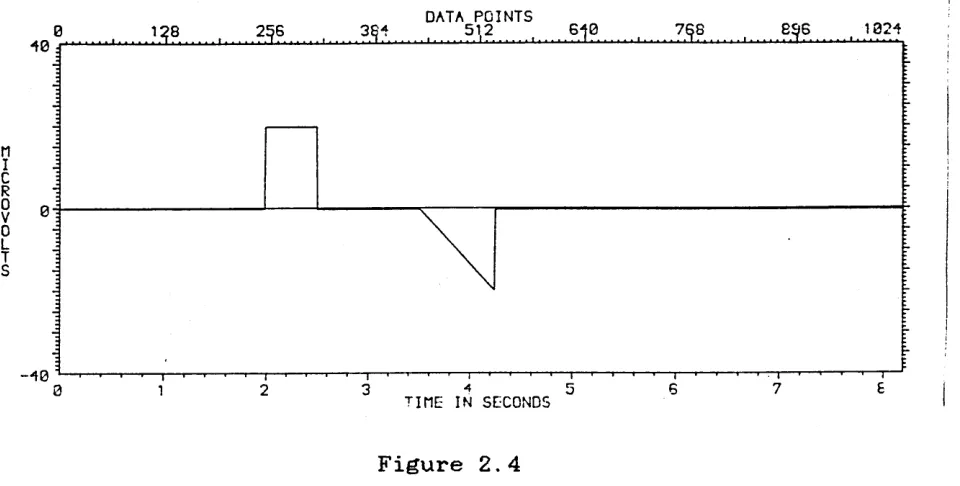
Figure 2.4

Simulated measured EEG which contains an OA and a response

X101

8 - J

7.

6

5. 4.

3. 2 .

1 .

BL. • II ■ . . . , 1 0 1 2 3 4 5 6 7 8 9

TIME (SEC)

Figure 2.5

The simulated EOG corresponding to the OA of Figure 2.4

The single component response model (dc ? 0) is shown in Figure 2.6.

-31-cn —i r~ o< o7 on *-i3 X101 > 3

-2

-3

-4

-5

-6

-7

-8

-9

O

_{9 1 2 3 4 5 6 7 8 9}

TinE (9EC )

;

Figure 2. 6

Linearly modelled response

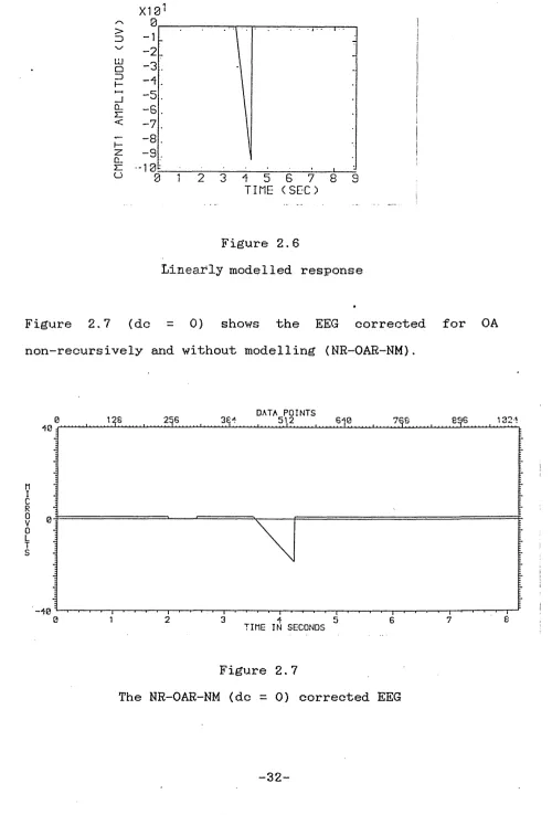
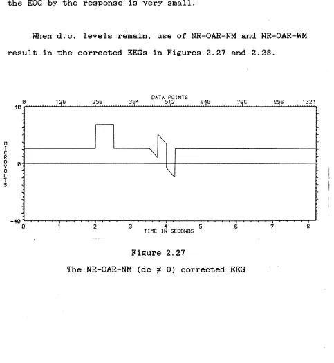
Figure 2.7 (dc = 0) shows the EEG corrected for OA non-recursively and without modelling (NR-OAR-NM).

DATA POINTS_{51,2 8^6}

TINE IN SECONDS

Figure 2.7

The estimated CNV differs from the known one only in that there is a small (1/jV) but constant level shift. The shape,

slope and maximum amplitude (relative to the baseline) are unchanged and there is an OA remnant (in the form of overcorrection of the measured EEG) of ljuV (5% of the original OA). The correction, with d.c. level removal, gave rise to the 9 (the estimated value) of 0.20984 , compared with the known value of 0.2, i.e., 4.92% in error.

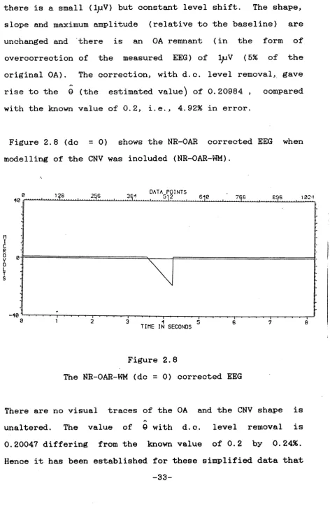
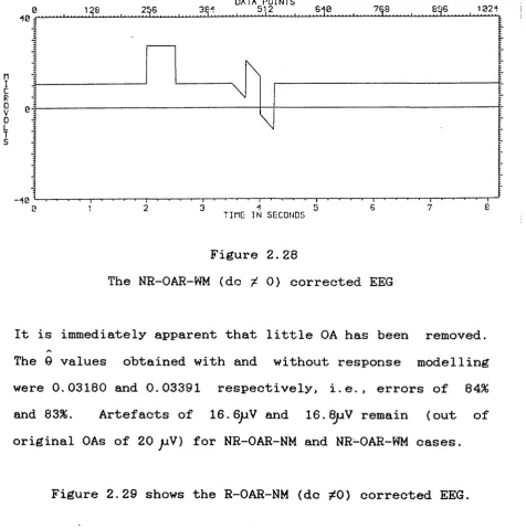
Figure 2.8 (dc = 0 ) shows the NR-OAR corrected EEG when modelling of the CNV was included (NR-OAR-WM).

DATA POINTS

51,2

f1_I

C

R0

V

0

L T S

-40

TIME IN SECONDS

Figure 2.8

The NR-OAR-WM (dc = 0) corrected EEG

There are no visual traces of the OA and the CNV shape is

-a.

unaltered. The value of 0 with d.c. level removal is 0.20047 differing from the known value of 0.2 by 0.24%. Hence it has been established for these simplified data that

-33-successful OAR can be achieved non-recursively provided the response is modelled.

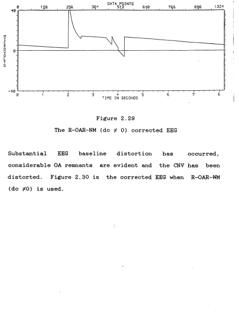
Figure 2.9 (dc = 0 ) shows the corrected EEG obtained

using the recursive method, but with no modelling

(R-OAR-NM).

512

n

I

r

R0

V

0

L T S

TIME IN SECONDS

Figure 2.9

The R-OAR-NM (dc = 0) corrected EEG

A vestige of OA remains varying from +2.8juV to -0.7juV, relative to the EEG baseline. It can also be observed that there exists a small difference in pre- and post-OA EEG baseline of ~0.5jjV. It appears that the CNV is unaltered.

addition the pre- and post-OA baseline difference of Figure 2.9 has been eliminated.

Figure 2.10 (dc = 0 ) is a plot of 0 agains number for the R-OAR-NM case showing a variation of during the record which accounts for the pre- and EEG baseline difference observed in Figure 2.9.

co C£

LU

1—

LU

H

< O' <

a.

LU

f—

2= I—

CO LU

35 xlO

30_

25.

20

-5 3

TIME (SEC)

CNVNCT1

BATCH

THETA 1

sample 0 value post-OA

0

.1917

Figure 2.10

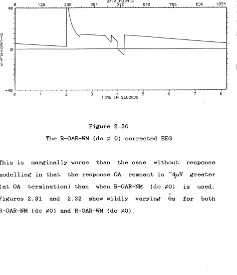
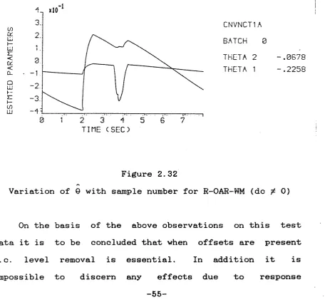
The following observations can be made: the abrupt change in 0 at t = 2 corresponds to the onset of OA; the more gradual increase in 0 commences in the vicinity of the start of the CNV (there being a slight delay ~0.2s); the change in sign of the slope of 0 occurs at CNV termination. Figure 2. 11 (dc = 0) shows the R-OAR-WM case in which the second trace (labelled "THETA 2") is the estimate for the CNV model component parameter, the 0g of equation (2.25).

(j) C£

LU

I—

LU

2= <

CH

< CL

O

LU

h-21 I—00

LU -5.1

CNVNCT1

BATCH 0

THETA 2

THETA 1

.2095

.2001

Figure 2. 11

A

Variation of 0 with sample number for R-OAR-WM (dc = 0)

(/

)H

r~

o<

07

3n

»-in

Figure 2.12 (dc ^ 0) shows the NR-OAR-NM corrected EEG, derived from data from which the d.c. level has not been

removed.

DATA POINTS

51,2

T IME IN SECOND!

Figure 2.12

The NR-OAR-NM (dc * 0) corrected EEG

This is seen to exhibit neither OA remnant nor CNV shape modification. This was found to be the case for all processing options (NR-OAR-NM, NR-OAR-WM, R-OAR-NM and R-OAR-WM). The value of 0 obtained by NR-OAR-NM and NR-OAR-WM was identical and equalled 0.20034, i.e., 0.17% in error. Figure 2.13 (dc i- 0) shows the plot of 0 variation when R-OAR-NM was performed. An identical plot was obtained when modelling was applied (except, of course, for the addition of the estimate of 0g, the model component).

-37-CO

cm

LU I— LU Z= < Of <

CL

Q LU

CO

LU

35 xlO

30.

25i

20

____

-5

TIME (SEC)

CNVNCT1

BATCH 0

THETA 1

.2003

Figure 2.13

Variation of Q with sample number for R-OAR-NM (dc 0)

For these simple data, the conclusions are that the response must be modelled if the d.c. levels of the data have been removed, and that response modelling gives good results in all cases.

( v -_{s Vn}

s(i) = < v

Vs.V + v _{s n}

N-l

i = 2,6,10,...,N-7,N-3 i.e. ---- terms

4

N+l

i = 1,3,5,...,N-2,N i.e. ---- terms 2

N-l

i = 4,8,12,...,N-5, N-l i.e. --- terms

4

- (2.27)

or for no 'noise':

s( i) = v i = 1, 2,3,. . . , N -(2.28)

The above are depicted in Figure 2.14.

\/

/ / /

N-2 N - l

N

Figure 2. 14

Illustration of effect of noise on sum of squares, J

Then for no 'noise':

-39-J = X O(i)]2 -

Nv2

i=l

-(2.29)

And when ’noise-’ is present:

N+l

N-l

N-l

2

4

4

N-l

(2.30)

2

Then comparing (2.29) and (2.30)

must always be greater

than J. Hence any given non-random response in the EEG will

have a greater effect on J than J .

_n

2.5.1.2 SEPARATE 0A AND A RESPONSE HAVING AN ADDITIONAL 0A

In the following d.c. levels have been removed from the

data yielding Figures 2.15, 2.17 - 2.21.

The remaining figures were obtained from data possessing

d.c, levels.

in —i r~ o < o n 3

DATA POINTS

1321

ZSi 138

-10

0 I 2 3 1 7 8

TINE IN SECONDS 5 6

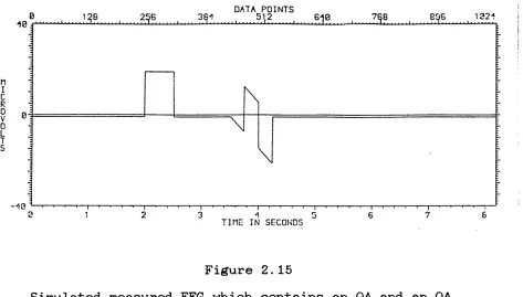
Figure 2.15

Simulated measured EEG which contains an OA and an OA superimposed on the response (do = 0)

The EOG causing the OAs is given in Figure 2.16 (do 5*0).

X 1 0 1

10, _

> ZD 9 r... A M P L I T U D E ( ₈ 7 6 5 4 3 -CD O LLi 2 1

_1 0 1 1 1 :

> _{0 1 2 3 5 6 7 8 9} T I M E ( S E C )

Figure 2.16

The simulated EOG (do f 0) corresponding to the OAs of

Figure 2.15

-41-tn

-H

-o

co

To

n-o

Using NR-OAR-NM gives the corrected EEG of Figure 2. 17 (dc =

0).

DATA POINTS

8^6

0 - j =

TinE- IN SECONDS

Figure 2.17

The NR-OAR-NM (dc = 0) corrected EEG

Incomplete removal of both OAs is observed, there remaining 13% of the original OA in each case. With NR-OAR-WM (dc = 0) the corrected EEG showed no trace of either OA, i.e., it

A

DATA POINTS_{SI, 2}

M_I

C R

0

V

0

L T S

TinE IN SECONDS

Figure 2.18

The R-OAR-NM (dc = 0) corrected EEG

The first OA is

initially

tp -m o <o xi o *-<r r

DATA POINTS

2^6

0 2 3 4 5

TINE IN SECONDS S 7 £

Figure 2.19

The R-OAR-WM (dc = 0) corrected EEG

The variations of 9 with sample number for R-OAR-NM (dc = 0) and R-OAR-WM (dc = 0) are shown in Figures 2.20 and 2.21 respectively.

to O' LU I— UJ z: < O' < CL QHI I—n t— to LU

35

30.

25.

-5.4

TIME (SEC)

CNVNCT1

BATCH 0

C

NVNCT1

BATCH 0

THETA 2

.2087

THETA 1

.1974

Figure 2.21

Variation of 6 with sample number for R-OAR-WM (dc = 0)

In the former 9 suffers a step change at the rising edge of the first OA with another rapid change starting at the rising edge of the second OA. The final values of 9 of 0.1492 was in error by 25.4% but between the rising edges of

/**

the two OAs 9 was much closer to the true value of 0.2. With response modelling the OAs cause much smaller change in 9 which, as expected for this one type of artefact, is more nearly constant, the final value of 0.1974 being within 1.3% of the true value. It is to be concluded once more that efficient OAR requires response modelling which also overcomes the response distortion introduced by R-OAR (Figures 2.18 and 2.19).

Study of the NR-OAR-NM, NR-OAR-WM, R-OAR-NM and R-OAR-WM corrected EEGs, in which d.c. levels remain,- were similar to their d.c. level-removed counterparts, excepting

LO

35 xlO

30_

25..

----5i

5

6

7

0 2

3

that their baselines remained at zero. The non-recursive estimates of 9 with and without response modelling were 0.19863 {0.1% in error) and 0.16379 (22.1% in error) respectively. Figure 2.22 shows the 9 variation with sample number for R-OAR-NM (dc j- 0).

co C£ LU 1— LU H <

C£

<

Q_

O LU h-07 LU

30 xlO

25.

20

-5 -10.:

TIME (SEC)

C

NVNCT1

BATCH 0

THETA 1

.1481

Figure 2.22

Variation of 9 with sample number for R-OAR-NM (dc ^ 0)

2.5.1.3 CO

NTAMINATION OF THE EOG BY THE RESPONSE

Contamination of the EOGs by background EEG or by the

response (IFEACHOR et al, 1986a; JERVIS et al, 1988) is

another problem found in practice.

This causes partial

correlation between the EOGs and the measured EEG which

leads to incorrect estimates of the 9 .s and hence of the

true (background) EEG and the responses. Thus the term

x.(i) in equation (2.13) is replaced by x.'"(i) where:

Xj’(i) = xj(i) + KjlEEGt (i) + Kj2CNV(i) -(2.31)

where

and K^2 are transmission coefficients indicating

contamination of the EOG by the true EEG and response

respectively. This situation was investigated by simulation

in which, as a simplification, K., was set to zero. A value

of K^2 =0.2 was introduced. To investigate the conflicting

results of Sections 2.5.1.1 and 2.5.1.2 regarding d.c. level

removal offsets of +10juV and -20juV were introduced into the

simulated measured EEG and EOG respectively.

The simulated measured EEG and EOG are given in Figures

2.23 and 2.24 respectively.

-47-DATA POINTS

bl,2

1 3 £

fl_I C R0 V 0 L T S

0 2 3 4 5 6 7 s

TINE IN SECONDS

Figure 2.23

Simulated EEG which contains an OA and an OA superimposed on a response, possesses an offset and in which dc 1 0

> ZD \/ o ZD Cl C< CD O LLi

X1

8

3

0

-2.

-3

3 1

2 3 * 1 5 6 7 8 9

TIME (SEC)

Figure 2.24

They both include d.c.

levels and show the offsets

introduced. The EEG was corrected for all four O

AR methods,

i.e., non-recursive/recursive and with/without response

modelling, in which d.c. levels were removed. The resultant

corrected EEGs were compared with the corresponding

waveforms of Section 2.5.1.2 (i.e.,

in which no

contamination of the EOGs occurred). Each pair of waveforms

were very similar, i.e., the sequence of correction methods

NR-OAR-NM, NR-OAR-WM, R-OAR-NM and R-OAR-WM yielded the same

waveforms as these shown in Figures 2.17, 2.8, 2.18 and 2.19

A

respectively. The values of © obtained for NR-OAR-NM and

NR-OAR-WM were 0.17865 (11.7% in error) and 0.19889 (0.7% in

error).

The corresponding estimates of 9 for no

contamination of the EOG (Section 2.5.1.2) were 0.17389 and

0.19863, i.e., differences of < 1.6% (for NR-OAR-NM) and <

0.04% (for

NR-OAR-WM)

between

contaminated

and

uncontaminated EOGs.

The © variations for R-OAR-NM and

R-OAR-WM are shown in Figures 2.25 and 2.26.