http://www.scirp.org/journal/ojop ISSN Online: 2325-7091
ISSN Print: 2325-7105
Intermodal Freight Network Design for
Transport of Perishable Products
Maxim A. Dulebenets*, Eren E. Ozguven, Ren Moses, Mehmet B. Ulak
Department of Civil & Environmental Engineering, Florida A&M University-Florida State University, Tallahassee, FL, USA
Abstract
The amount of perishable products transported via the existing intermodal freight networks has significantly increased over the last years. Perishable products tend to decay due to a wide range of external factors. Supply chain operations mismanage-ment causes waste of substantial volumes of perishable products every year. The he-retofore proposed mathematical models optimize certain supply chain processes and reduce decay of perishable products, but primarily deal with local production, in-ventory, distribution, and retailing of perishable products. However, significant quantities of perishable products are delivered from different continents, which shall increase the total transportation time and decay potential of perishable products as compared to local deliveries. This paper proposes a novel optimization model to de-sign the intermodal freight network for both local and long-haul deliveries of pe-rishable products. The objective of the model aims to minimize the total cost asso-ciated with transportation and decay of perishable products. A set of piecewise ap-proximations are applied to linearize the non-linear decay function for each perisha-ble product type. CPLEX is used to solve the properisha-blem. Comprehensive numerical experiments are conducted using the intermodal freight network for import of the seafood perishable products to the United States to draw important managerial in-sights. Results demonstrate that increasing product decay cost may significantly change the design of intermodal freight network for transport of perishable products, cause modal shifts and affect the total transportation time and associated costs.
Keywords
Freight Transportation, Network Design, Perishable Products, Shelf Life, Optimization
1. Introduction
Many of products transported via intermodal freight networks are perishable in their
How to cite this paper: Dulebenets, M.A., Ozguven, E.E., Moses, R. and Ulak, M.B. (2016) Intermodal Freight Network Design for Transport of Perishable Products. Open Journal of Optimization, 5, 120-139.
http://dx.doi.org/10.4236/ojop.2016.54013
Received: October 2, 2016 Accepted: December 27, 2016 Published: December 30, 2016
Copyright © 2016 by authors and Scientific Research Publishing Inc. This work is licensed under the Creative Commons Attribution International License (CC BY 4.0).
http://creativecommons.org/licenses/by/4.0/
nature. Perishable products (such as agricultural products, meat, fish, shellfish, phar-maceutical products, etc.) are sensitive to a wide range of different factors, which in-clude but are not limited to temperature, barometric pressure, humidity, air composi-tion and transportacomposi-tion time [1] [2] [3]. The demand for perishable products has been continuously growing. According to National Oceanic and Atmospheric Administra-tion (NOAA), the total volume of seafood perishable products, which have been im-ported to the United States (US), increased by 7.6% over the last five years and reached 2.7 million tons in 2015 [4]. Furthermore, the value of seafood perishable products, which have been delivered to the US, increased by 13.2% over the last five years and reached $19.2 billion in 2015 [4]. Peeled frozen shrimp, frozen tilapia fillet, and fresh Atlantic farm raised salmon are the top three seafood perishable products, which are imported to the US mainly from India, China, and Chile respectively [4].
Refrigerated containers (a.k.a., “reefers”) are generally used for transport of perisha-ble food products. Reefers are aperisha-ble to maintain a certain temperature and decrease phy-siological, microbiological, and physical changes in the perishable product [5]. Reefers allow slowing down decay of perishable products, but do not completely eliminate it. Due to temperature deviations within the containers perishable products may continue ripening. For example, the daily ripening rate of bananas may increase up to ~75% from increasing the temperature inside a given container from 15˚C to 20˚C [5]. Each perishable product must be delivered via the freight transportation network to the cus-tomer before the end of its “shelf life”, which represents the number of remaining days for a given perishable product to be of an acceptable quality for consumption. To ob-tain the information regarding the perishable product quality throughout the transpor-tation process, many freight carries rely on the advanced information technologies. Ra-dio-Frequency Identification (RFID) is one of the most frequently used technologies for traceability of perishable products within containers [3] [5] [6].
case of operations mismanagement is significantly higher for long-haul deliveries and compared to local deliveries.
Therefore, there is a need for more comprehensive models to design the intermodal freight network that would allow selection of the appropriate transportation routes and transportation modes for shipments with perishable products. This paper aims to fill the existing gap in the state-of-the-art and proposes a novel optimization model for ef-ficient management of supply chains with perishable products that can be used for both local and long-haul deliveries. The objective of the model aims to minimize the total cost associated with transportation and decay of perishable products. A set of piecewise approximations are applied to linearize the non-linear decay function for each perisha-ble product type, and the resulting mixed integer linear properisha-blem is solved using CPLEX. Numerical experiments are performed using the intermodal freight network for import of the seafood perishable products to the US. The rest of the manuscript is organized as follows. The next section provides a detailed problem description, while the third tion presents the mathematical model and the solution methodology. The fourth sec-tion describes a set of numerical experiments conducted to evaluate performance of the adopted solution methodology and reveal important managerial insights using the de-veloped mathematical model. The last section summarizes the study findings and pro-poses directions for the future research.
2. Problem Description
This section of the paper focuses on description of the main problem features, includ-ing the followinclud-ing: 1) network elements; 2) cargo transfer within intermodal terminals; 3) perishability modeling; 4) shelf life of perishable shipments; and 5) decisions.
2.1. Network Elements
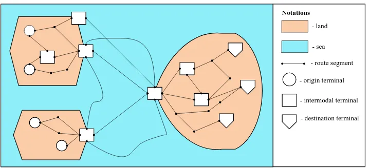
An example of the intermodal freight network is presented in Figure 1. Let P=
{
1,,k}
be a set of perishable shipments. Each perishable shipment is assumed to have an origin terminal and a destination terminal (see Figure 1). The origin and destination termin-als of the perishable shipments are connected with a set of transportation routes
{
1, ,}
R= m . Each route is divided in a set of route segments S=
{
1,,o}
. At eachsegment the shipping company is able to select a transportation mode (i.e., sea, air, rail, truck, etc.) out of the set of modes M=
{
1,,w}
. It is assumed that availability ofmodes varies from one route segment to another (e.g., at route segments passing through sea the shipping company can transport the perishable shipment either by sea or air, while at land route segments the shipping company can transport the perishable shipment either by air or rail or truck). The transportation time tTpsm,p∈P s, ∈S m, ∈M
(measured in hours) and associated cost T , , ,
psm
c p∈P s∈S m∈M (measured in USD)
Figure 1. Intermodal freight network example.
2.2. Cargo Transfer within Intermodal Terminals
A transfer of perishable shipments from one mode to another occurs within the inter-modal terminals (see Figure 1). The handling time at the intermodal terminal H ,
psm
t
, ,
p∈P s∈S m∈M (measured in hours) and associated cost cHpsm,p∈P s, ∈S m, ∈M
(measured in USD) are assumed to vary depending on the type of a perishable ship-ment (captured by index p), route segment (captured by index s), and mode selected
for transport at a given route segment (captured by index m). The latter allows
tack-ling the change in handtack-ling time and cost of a given perishable shipment due to its size (e.g., increasing size of shipments will increase the handing time), mode availability depending on the route segment selected, and required resources for transfer of a cargo from one mode to the other.
2.3. Perishability Modeling
The quality of perishable products within each shipment is assumed to deteriorate over time. Increase in the total transportation time (which includes the total transportation time along the route segments of the selected route and the total handling time at the intermodal terminals) negatively affects freshness of products in each shipment. Each perishable shipment is assumed to be homogenous (i.e., each shipment is composed of perishable products of the same nature, which deteriorate at the same rate over time). Based on the available literature, the quality of a perishable product in shipment p at a given time T can be estimated based on the following equation [2], [3], [16], [17]:
0 e p pT T
p p
Q =Q −ϕ ∀ ∈p P (1)
where:
T p
Q —is the quality of a perishable product in shipment p at time T (i.e., once it
is unloaded at the destination terminal-%); 0
p
Q —is the quality of a perishable product in shipment p at time 0 (i.e., once it
is loaded at the origin terminal-%);
p
ϕ —is the decay rate of a perishable product in shipment p (hour−1);
Notations
- land
- sea
- origin terminal
- intermodal terminal
p
T —is the total transportation time of perishable shipment p from the origin ter-minal to the destination terter-minal (hours).
The decay rate ϕp depends on the nature of a perishable product in shipment p.
For example, a typical decay rate for the meat product is ϕmeat =0.0067 hour−1, while a fresh vegetable product typically decays at a rate ϕveg=0.0216 hour−1[2]. Based on Equation (1) the decay of a perishable product in shipment p D
(
p,p∈P−%)
can be further computed as:(
)
0
0 0 0
0 0 0
1 e e
1 e
p p p p
p p T
T T
p T
p p p p
p
p p p
Q
Q Q Q Q
D p P
Q Q Q
ϕ ϕ
ϕ
− −
−
−
− −
= = = = − ∀ ∈ (2)
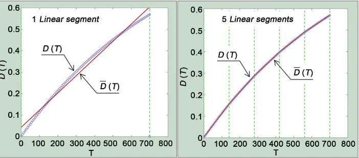
Note that decay function Dp is non-linear and can be linearized using its piecewise
linear approximation Dp. Figure 2 demonstrates examples of piecewise linear
ap-proximations for a non-linear product decay function 0.0012 1 e Tp p
D = − − . The decay rate
of a perishable product, transported in refrigerated containers was assumed to be
0.0012
p
ϕ = hour−1 (i.e., ≈15 ÷ 20% of the decay rate, when the product is transported
in a regular container [2]). The total transportation time was assumed to be up to 700 hours (i.e., Tp≤700 hours ≈ 30 days). We observe that increasing number of linear
segments in the piecewise linear approximation improves accuracy of Dp function,
but may incur an increasing computational time (due to increase in the number of va-riables in the optimization model). A tradeoff between the approximation accuracy vs. computational time will be analyzed in the numerical experiments section.
Let Lp =
{
1,,hp}
,p∈P be a set of linear segments in piecewise linearapproxi-mation Dp. Let gpl =1 if linear segment l is selected to approximate the decay
function for a perishable product in shipment p. Let TVplb,p∈P l, ∈Lp and , e pl
TV
, p
p∈P l∈L be the transportation time value of a perishable product in shipment p at the beginning and the end of linear segment l respectively. Let SLpl,p∈P l, ∈Lp
and INpl,p∈P l, ∈Lp be the slope and the intercept of linear segment l for the
[image:5.595.200.551.534.689.2]de-cay function of a perishable product in shipment p respectively. Let M0 be a large positive number. Then the approximated decay of a perishable product in shipment p can be estimated using the following set of equations:
1
p pl l L
g p P
∈
= ∀ ∈
∑
(3),
b
pl pl p p
TV g ≤ ∀ ∈T p P l∈L (4)
(
)
0 1 ,
e
pl pl p p
TV +M −g ≥ ∀ ∈T p P l∈L (5)
(
)
0 1 ,
p pl p pl pl p
D ≥SL T +IN −M −g ∀ ∈p P l∈L (6)
Constraints set (3) indicates that only one segment of the piecewise function should be selected for approximation of the decay function for a perishable product in a given shipment. Constraints sets (4) and (5) define the range of the total transportation time values, when a given linear segment should be used to approximate the decay function for a perishable product in a given shipment. Constraints set (6) computes the ap-proximated decay of a perishable product in a given shipment at the destination ter-minal.
2.4. Shelf Life of Perishable Shipments
As discussed in the introduction section of the paper, perishable products should be de-livered to their destinations before the end of their shelf lives in order to be of an ac-ceptable quality for the consumers. This study captures the latter operational aspect by imposing the following constraints set for each perishable shipment p:
max
p p
T ≤T ∀ ∈p P (7)
where: max
p
T —is the shelf life of a perishable product in shipment p (hours).
Constraints set (7) ensures that each perishable shipment will be delivered to its des-tination before the end of its shelf life.
2.5. Decisions
In this problem, the shipping company needs to make the following two major deci-sions: a) select a route for transportation of each perishable shipment; and b) choose a transportation mode at each segment of the selected route for each perishable shipment. Both decisions should account for a number of factors such as: 1) transportation mode availability at a given route segment; 2) increasing transportation cost for selection of faster transportation mode (e.g., transportation time by air will be smaller than by sea, but will incur higher transportation costs); 3) handling time at the intermodal terminals depending on selected mode (e.g., loading containers on a vessel may take longer as compared to loading containers on a train); 4) increasing product decay costs due to increasing total transportation time; 5) decay rate of a perishable product in a given shipment (e.g., higher decay rate will require the shipping company to select faster transportation modes at route segments to ensure that the products will be delivered to their destination terminal before the end of their shelf life).
3. Mathematical Model
mixed integer mathematical model for the intermodal freight network design problem with perishable products.
3.1. Notations Sets
}
{
1, ,P= k Set of perishable shipments
}
{
1, ,R= m Set of available routes
}
{
1, ,S= o Set of route segments
}
{
1, ,M= w Set of available transportation modes
}
{
1, , ,p p
L = h p∈P Set of linear segments in the piecewise decay function for perishable shipment p
Decision variables
, ,
pr
y p∈P r∈R =1 if route r is selected for transportation of perishable shipment
p (=0 otherwise)
, , ,
psm
x p∈P s∈S m∈M =1 if transportation mode m is selected at route segment s
for transportation of perishable shipment p (=0 otherwise)
Auxiliary variables
, p
T p∈P Total transportation time of perishable shipment p (hours)
, ,
pl p
g p∈P l∈L =1 if linear segment l is selected to approximate the decay
function for a perishable product in shipment p (=0 otherwise)
, p
D p∈P Approximated decay of a perishable product in shipment p (%)
Parameters
k Number of perishable shipments (shipments)
m Number of available routes (routes)
o Number of route segments (segments)
w Number of available transportation modes (modes)
, p
h p∈P Number of linear segments in the piecewise decay function for
perishable shipment p (segments)
, , ,
T psm
c p∈P s∈S m∈M Transportation cost of perishable shipment p at route segment s
by mode m (USD)
, , ,
H psm
c p∈P s∈S m∈M Handling cost of perishable shipment p to be transported at
route segment s by mode m (USD)
, D p
Continued
, , ,
T psm
t p∈P s∈S m∈M Transportation time of perishable shipment p at route segment s
by mode m (hours)
, , ,
H psm
t p∈P s∈S m∈M Handling time of perishable shipment p to be transported
at route segment s by mode m (hours)
max
, p
T p∈P Shelf life of a perishable product in shipment p (hours)
, p
q p∈P Quantity of perishable products in shipment p (products)
0
, p
Q p∈P Quality of a perishable product in shipment p at time 0 (%)
, , ,
prs
z p∈P r∈R s∈S =1 if route segment s belongs to route r for transport of
perishable shipment p (= 0 otherwise)
, ,
pr
RA p∈P r∈R =1 if route r is available for transport of perishable shipment p
(= 0 otherwise)
, , ,
psm
MA p∈P s∈S m∈M =1 if mode m is available at route segment s for transport
of perishable shipment p ( = 0 otherwise)
, ,
b
pl p
TV p∈P l∈L Transportation time value for a perishable product in
shipment p at the beginning of linear segment l (hours)
, ,
e
pl p
TV p∈P l∈L Transportation time value for a perishable product in
shipment p at the end of linear segment l (hours)
, ,
pl p
SL p∈P l∈L Slope of linear segment l for the decay function of a
perishable product in shipment p
, ,
pl p
IN p∈P l∈L Intercept of linear segment l for the decay function of a
perishable product in shipment p
0
M Large positive number
3.2. Model Formulation
The mixed integer mathematical model for the intermodal freight network design problem with perishable products (IFNDP) can be formulated as follows:
IFNDP:
(
)
0min Tpsm Hpsm psm Dp p p p
p P s S m M p P
c c x c q Q D
∈ ∈ ∈ ∈
∑∑ ∑
+ +∑
(8)Subject to:
1
pr r R
y p P
∈
= ∀ ∈
∑
(9),
pr pr
y ≤RA ∀ ∈p P r∈R (10)
, ,
psm pr prs
r R
x y z p P s S m M
∈
=
∑
∀ ∈ ∈ ∈ (11), ,
psm psm
x ≤MA ∀ ∈p P s∈S m∈M (12)
(
H T)
p psm psm psm
s S m M
T t t x p P
∈ ∈
=
∑ ∑
+ ∀ ∈ (13)max
p p
1
p pl l L
g p P
∈
= ∀ ∈
∑
(15),
b
pl pl p p
TV g ≤ ∀ ∈T p P l∈L (16)
(
)
0 1 ,
e
pl pl p p
TV +M −g ≥ ∀ ∈T p P l∈L (17)
(
)
0 1 ,
p pl p pl pl p
D ≥SL T +IN −M −g ∀ ∈p P l∈L (18)
{ }
, , , , , 0,1 , , , ,
pr psm pl prs pr psm p
y x g z RA MA ∈ ∀ ∈p P r∈R s∈S m∈M l∈L (19)
, , , , p, p
k m o w h q ∈ ∀ ∈N p P (20) max 0
0
, , T , H , D, T , H , , , b, e, , , , , ,
p p psm psm p psm psm p p pl pl pl pl p
T D c c c t t T Q TV TV SL IN M ∈ ∀ ∈R+ p P s∈S m∈M l∈L (21)
In IFNDP, the objective function (8) aims to minimize the total cost associated with transportation of perishable shipments, handling of perishable shipments at the inter-modal terminals, and decay of perishable shipments throughout the transportation process. Constraints set (9) ensures that only one route should be selected for transport of a given perishable shipment. Constraints set (10) indicates that the route for trans-port of a given perishable shipment should be selected only from the routes available for transport of that particular shipment. Constraints set (11) ensures that a given pe-rishable shipment should be transported along all the segments of the selected route. Constraints set (12) ensures that the mode for transport of a given perishable shipment should be selected only from the modes available for transport of that particular ship-ment at a given route segship-ment. Constraints set (13) estimates the total transportation time of a given perishable shipment. Constraints set (14) ensures that each perishable shipment will be delivered to its destination before the end of its shelf life. Constraints set (15) indicates that only one segment of the piecewise function should be selected for approximation of the decay function for a perishable product in a given shipment. Constraints sets (16) and (17) define the range of the total transportation time values, when a given linear segment should be used to approximate the decay function for a perishable product in a given shipment. Constraints set (18) computes the approx-imated decay of a perishable product in a given shipment at the destination terminal. Constraints sets (19)-(21) define the nature of IFNDP variables and parameters. 3.3. Solution Methodology
Application of the piecewise linear approximations for the product decay functions al-lows formulating IFNDP as a mixed integer linear mathematical model, which can be solved using commercial optimization solvers (e.g., CPLEX) within an acceptable computational time even for large size problem instances (as will be discussed in the numerical experiments section).
4. Numerical Experiments
4.1. Input Data Generation
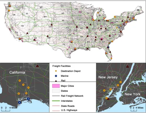
The numerical data for computational experiments were generated based on the aca-demic literature and publicly available resources [19]-[30]. A total of top ten seafood perishable product types, based on the overall volumes imported to the US, were con-sidered in this study. The top origin country and the top five US destinations (based on the overall volumes) for each perishable product type were retrieved using the data provided by NOAA [4] and are presented in Table 1.
[image:10.595.50.550.301.687.2]The intermodal freight network for transport of perishable products (see Figure 3) included 5 marine terminals, 40 rail terminals, and 50 destination depots. Locations of the intermodal terminals were retrieved using the data provided by the Intermodal As-sociation of North America [19]. Each shipment was assumed to originate at one of the marine terminals of the top exporting country. A total of 50 possible routes were con-sidered for each origin-destination pair. The intermodal freight network was composed of 350 route segments. Since seafood perishable products are rarely transported
Table 1. Origins and destinations by product type.
a/a Product Top Exporting
Country Top US Destinations
1 SHRIMP WARM-WATER PEELED FROZEN INDIA NEW YORK, NY; LOS ANGELES, CA; MIAMI, FL; SAVANNAH, GA; HOUSTON-GALVESTON, TX
2 TILAPIA (OREOCHROMIS SPP.) FILLET FROZEN CHINA BALTIMORE, MD; BOSTON, MA; BUFFALO, NY; CHARLESTON, SC; CHICAGO, IL
3 SALMON ATLANTIC FILLET FRESH FARMED CHILE HOUSTON-GALVESTON, TX; DALLAS-FORT WORTH, TX MIAMI, FL; LOS ANGELES, CA; NEW YORK, NY;
4 CATFISH (PANGASIUS) FILLET FROZEN VIET NAM BALTIMORE, MD; BOSTON, MA; CHARLESTON, SC; CHICAGO, IL; CLEVELAND, OH
5 SALMON ATLANTIC FRESH FARMED CANADA SEATTLE, WA; PORTLAND, OR; DETROIT, MI; BUFFALO, NY; OGDENSBURG, NY
6 TUNA ALBACORE IN ATC (OTHER) NOT IN OIL OVER QUOTA THAILAND BALTIMORE, MD; BOSTON, MA; CHARLESTON, SC; CHICAGO, IL; DALLAS-FORT WORTH, TX
7 SHRIMP FROZEN OTHER PREPARATIONS THAILAND LOS ANGELES, CA; TAMPA, FL; NEW YORK, NY; SAVANNAH, GA; NORFOLK, VA
8 CRAB SNOW FROZEN CANADA PORTLAND, OR; DETROIT, MI; SAINT ALBANS, VT; OGDENSBURG, NY; BUFFALO, NY
9 GROUNDFISH COD NSPF FILLET FROZEN CHINA NORFOLK, VA; BOSTON, MA; SEATTLE, WA; NEW YORK, NY; LOS ANGELES, CA
10 SHRIMP BREADED FROZEN CHINA LOS ANGELES, CA; TAMPA, FL; MIAMI, FL; NEW YORK, NY; NORFOLK, VA
by air, a total of three transportation modes were considered: 1) road; 2) rail; and 3) sea (i.e., a set of modes is M =
{
road; rail; sea}
). The latter does not limit generality of theproposed model, and the air mode can be included when modeling transport of other perishable products (e.g., pharmaceutical products, human specimens, organs, etc.).
The transportation cost of a perishable shipment was assigned based on the unit transportation cost by mode ( T
m
uc , USD per mile) and length of a route segment (ds,
miles) as follows: cTpsm =uc dmT s
(
1+U[
0.1; 0.2]
)
∀ ∈p P s, ∈S m, ∈M (USD), where U—is a notation used for uniformly distributed pseudorandom numbers. The han-dling cost of a perishable shipment was generated based on the average hanhan-dling costby mode ( H
m
ac , USD) as follows: H H
(
1[
0.1; 0.2]
)
, ,psm m
c =ac +U ∀ ∈p P s∈S m∈M
(USD). The transportation time along route segments of a perishable shipment was calculated based on the route segment length and the average speed by mode (vm,
mph) as follows:
(
[
]
)
, ,1 0.1; 0.2
T s
psm m
d
t p P s S m M
v U
= ∀ ∈ ∈ ∈
+ (hours). The handling
time of a perishable shipment at the intermodal terminals was computed based on the average handling time by mode ( H
m
at , hours) as follows:
[
]
(
1 0.1; 0.2)
, ,H H
psm m
t =at +U ∀ ∈p P s∈S m∈M (hours). Note that the random terms
(assigned using the uniform distribution) in T psm
c , H
psm
c , T psm
t , and H psm
t formulas
[
40; 60]
D p
c =U ∀ ∈p P (USD). The shelf life of a perishable product in a given
ship-ment was generated as max
[
]
840; 960
p
T =U ∀ ∈p P (hours). The quantity of perishable
products in each shipment was set to qp=U
[
1000; 2000]
∀ ∈p P (products). Thequality of products in each perishable shipment at the origin terminal was assumed to be 100% (i.e., 0
100%
p
Q = ∀ ∈p P). The decay rate of a perishable product in a given
perishable shipment was assigned as: ϕp=U
[
0.0008; 0.0012]
∀ ∈p P (hour−1). Valuesof the parameters used for the input data generation are presented in Table 2.
All numerical experiments were conducted on a Dell Intel(R) CoreTM i7 Processor
with 32 GB of RAM. IFNDP mathematical model was coded in General Algebraic Modeling System (GAMS, [31]) and solved using CPLEX. Piecewise linear approxima-tions for product decay funcapproxima-tions were developed using MATLAB 2016a [32].
4.2. Solution Methodology Evaluation
As discussed in section 2.3 of the paper, increasing number of segments in the piece-wise approximation increases accuracy of estimating the product decay values and the objective function itself, but may increase the computational time required to solve IFNDP mathematical model. A total of 25 problem instances were generated using the retrieved data, described in section 4.1, to analyze the latter tradeoff by changing the number of perishable shipments to be transported (from 2 to 10 shipments) and the number of linear segments in the piecewise approximation (from 10 to 100 segments). Detailed information regarding each shipment is provided in Table 3, including the following data: 1) shipment number; 2) perishable product type; 3) origin country; 4) US destination (randomly selected out of top five US destinations for a given product type); and 5) quantity of perishable products shipped. For example, the first shipment includes 1294 units/packages of shrimp warm-water peeled frozen and is imported from India to New York (NY).
[image:12.595.56.552.522.708.2]IFNDP was solved for each one of the developed problem instances, and results are presented in Table 4, including the following information: 1) instance number; 2)
Table 2.Numerical data.
Parameter Value References
Unit transportation cost by mode— T m
uc (USD/mile) [3.0; 2.0; 0.5] [20], [21]
Average handling cost by mode— H m
ac (USD) [400; 450; 500] [23] [24] [25]
Average speed by mode—vm (mph) [60; 40; 20] [8], [26], [27]
Average handling time by mode— H m
at (hours) [0.8; 0.9; 1.0] [24]
Decay cost for a perishable product in a given shipment— D p
c (USD) U[40; 60] N/A
Shelf life of a perishable product— max
p
T (hours) U[840;960] N/A
Quantity of perishable products—qp,p∈P (products) U[1000; 2000] N/A Decay rate of a perishable product—ϕp (hour
Table 3. Shipment characteristics.
Shipment Product Type Origin Destination Quantity
#1 SHRIMP WARM-WATER PEELED FROZEN INDIA NEW YORK, NY 1294
#2 TILAPIA (OREOCHROMIS SPP.) FILLET FROZEN CHINA BOSTON, MA 1012
#3 SALMON ATLANTIC FILLET FRESH FARMED CHILE MIAMI, FL 1253
#4 CATFISH (PANGASIUS) FILLET FROZEN VIET NAM BALTIMORE, MD 1470
#5 SALMON ATLANTIC FRESH FARMED CANADA DETROIT, MI 1694
#6 TUNA ALBACORE IN ATC (OTHER) NOT IN OIL OVER QUOTA THAILAND CHARLESTON, SC 1352
#7 SHRIMP FROZEN OTHER PREPARATIONS THAILAND TAMPA, FL 1329
#8 CRAB SNOW FROZEN CANADA BUFFALO, NY 1640
#9 GROUNDFISH COD NSPF FILLET FROZEN CHINA SEATTLE, WA 1498
#10 SHRIMP BREADED FROZEN CHINA NORFOLK, VA 1922
Table 4.Solution methodology performance.
Instance #Shipments #Segments #Variables 𝑨𝑨𝑨𝑨 𝑨𝑨𝑨𝑨∗ ∆
𝑨𝑨𝑨𝑨 𝑻𝑻𝑻𝑻, 106 USD 𝑻𝑻𝑻𝑻∗, 106 USD ∆𝑻𝑻𝑻𝑻 CPU, sec 1
1-2
10 2228 39.5733
39.5551
4.61E−04 6.6377
6.6360
2.52E−04 0.170
2 30 2268 39.5587 9.02E−05 6.6364 5.02E−05 0.172
3 50 2308 39.5571 5.04E−05 6.6362 2.76E−05 0.183
4 70 2348 39.5557 1.61E−05 6.6361 9.40E−06 0.197
5 100 2408 39.5556 1.28E−05 6.6361 6.99E−06 0.198
6
1-3
10 3340 39.6599
39.6411
4.75E−04 10.8365
10.8338
2.49E−04 0.199
7 30 3400 39.6432 5.34E−05 10.8341 2.81E−05 0.221
8 50 3460 39.6423 3.01E−05 10.8340 1.38E−05 0.224
9 70 3520 39.6417 1.57E−05 10.8339 8.34E−06 0.225
10 100 3610 39.6411 6.04E−07 10.8338 6.31E−08 0.242
11
1-5
10 5564 40.8238
40.8042
4.80E−04 19.5961
19.5912
2.45E−04 0.287
12 30 5664 40.8056 3.56E−05 19.5916 1.70E−05 0.308
13 50 5764 40.8052 2.47E−05 19.5915 1.18E−05 0.342
14 70 5864 40.8047 1.38E−05 19.5914 6.85E−06 0.358
15 100 6014 40.8046 9.37E−06 19.5913 4.50E−06 0.371
16
1-7
10 7788 42.6822
42.6633
4.43E−04 29.4200
29.4133
2.31E−04 0.390
17 30 7928 42.6642 2.04E−05 29.4136 1.02E−05 0.393
18 50 8068 42.6640 1.63E−05 29.4135 7.45E−06 0.396
19 70 8208 42.6639 1.32E−05 29.4135 6.74E−06 0.417
20 100 8418 42.6639 1.23E−05 29.4135 6.59E−06 0.418
21
1-10
10 11,124 42.2643
42.2482
3.81E−04 42.9171
42.9089
1.92E−04 0.440
22 30 11,324 42.2489 1.62E−05 42.9092 7.64E−06 0.463
23 50 11,524 42.2489 1.55E−05 42.9092 6.99E−06 0.473
24 70 11,724 42.2486 9.33E−06 42.9091 5.07E−06 0.486
[image:13.595.47.550.299.708.2]number of shipments; 3) number of linear segments in the piecewise approximations; 4) total number of variables in IFNDP mathematical model; 5) average over all shipments product decay estimated based on piecewise approximations—AD; 6) true average
product decay estimated based on the non-linear product decay functions—AD∗; 7)
average product decay gap— AD
AD AD
AD ∗
∗
−
∆ = ; 8) objective function value estimated
based on piecewise approximations—TC; 9) true objective function value estimated
based on the non-linear product decay functions at the solution provided by IFNDP—
TC∗; 10) objective function gap— TC
TC TC
TC ∗
∗
−
∆ = ; and 11) computation time.
We observe that increasing the number of segments in the piecewise function from 10 to 100 segments on average reduces the product decay and objective function gaps by 98.46% and increases the computational time only by 17.24%. Furthermore, the computational time over all the generated problem instances did not exceed 0.49 sec. The latter results demonstrate efficiency of the proposed solution approach, consider-ing the fact that relatively large size problem instances were analyzed with up to 12,024 variables. The computational time may increase for larger intermodal freight networks. Application of the developed mathematical model for larger intermodal freight net-works can be one of the future research directions of this study. Piecewise approxima-tions with 100 segments will be further adopted for analysis of the managerial insights.
4.3. Managerial Insights
This section of the paper demonstrates how the developed optimization model can be used to draw important managerial insights. A total of 10 scenarios were developed for the problem instance with 10 perishable shipments by increasing the product decay cost as follows: ( )1
[
1.1; 2.5]
D D
pi p i
c + =c U ∀ ∈p P (USD), where i—is the scenario number.
The generated product decay cost values for each perishable shipment and scenario are presented in Table 5. IFNDP was solved for each one of the generated product decay cost scenarios. Next this section elaborates on how increasing product decay cost af-fected the total miles traveled by each mode, total transportation time, decay of perish-able products, and associated transportation and product decay costs.
4.3.1. Total Miles Traveled by Mode
Figure 4.Total miles traveled by mode and scenario.
Table 5. Product decay cost by shipment and scenario (USD).
Shipment\Scenario 1 2 3 4 5 6 7 8 9 10
Shipment #1 55 127 203 271 340 410 482 545 613 682
Shipment #2 56 124 198 262 333 412 472 541 613 689
Shipment #3 54 134 194 265 333 402 475 550 611 688
Shipment #4 54 123 198 266 344 401 473 554 619 691
Shipment #5 53 132 203 272 338 408 478 542 621 682
Shipment #6 63 120 203 260 334 408 479 542 617 685
Shipment #7 62 125 197 272 344 407 474 553 610 682
Shipment #8 56 130 196 264 343 400 481 547 624 692
Shipment #9 57 129 194 264 333 410 481 552 617 685
Shipment #10 58 122 191 267 330 413 481 551 615 684
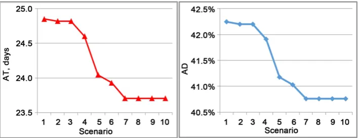
4.3.2. Total Transportation Time and Product Decay
Throughout the numerical experiments the average total transportation time
( )
ATand the average product decay
( )
AD over all perishable shipments were retrieved foreach one of the product decay cost scenarios. Results are illustrated in Figure 5, where we observe that increasing the product decay cost from 57 USD to 686 USD on average decreases the total transportation time of perishable shipments by 1.15 days. As dis-cussed in Section 4.3.1, decrease in the total transportation time was achieved by se-lecting a faster transportation mode for inland transport of perishable shipments (i.e., shipments were loaded on trucks instead of trains). Reduction in total transportation time yielded decrease in the average product decay by ≈1.5%.
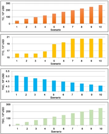
4.3.3. Cost Analysis
The scope of numerical experiments also included a detailed analysis of IFNDP cost components. The objective function and its components were estimated using the pro-posed mathematical model for each one the generated product decay cost scenarios. Results are presented in Figure 6, including the following cost components: 1) the total cost (i.e., objective function value)—TC; 2) the total cost of transporting perishable shipments along the route segments—TTC; 3) the total cost of handling perishable shipments at the intermodal terminals—THC; and 4) the total cost associated with de-cay of perishable products throughout the transportation process—TDC. It can be no-ticed that the total transportation cost increases with increasing product decay cost. The latter finding can be explained by the fact that the shipping company was required to select primarily trucks for inland transportation of perishable shipments to reduce the associated product decay, which incurred additional costs (as the unit transporta-tion cost by road was assigned to be higher as compared to the unit transportatransporta-tion cost by rail). Decrease in the total handling cost from selection of trucks can be justified by lower average handling costs that were assigned for handling perishable shipments from trucks than from trains at the intermodal terminals (400 USD/shipment vs. 450 USD/shipment respectively).
[image:16.595.196.551.546.683.2]Furthermore, numerical experiments show that the total decay cost is still increasing from one scenario to the other despite decrease in the actual decay of perishable pro-
Figure 6.Objective function components by scenario.
5. Conclusions and Future Research
The amount of perishable products transported via the existing intermodal freight networks significantly increased over the last decade. Due to operations mismanage-ment within supply chains with perishable products drastic losses associated with the product decay have been reported. Moreover, published to date mathematical models primarily optimize supply chain processes that deal with local production, inventory, distribution, and retailing of perishable products. Nevertheless, many perishable prod-uct types are imported from different continents, which increases the total transporta-tion time and decay potential as compared to local deliveries. Unlike previous models in the literature, this paper proposed a novel mathematical model to design the inter-modal freight network for both local and long-haul deliveries of perishable products. The objective aimed to minimize the total cost associated with transport and decay of perishable products. A set of piecewise approximations were adopted to linearize the non-linear decay function for each perishable product type. CPLEX was used to solve the problem. Numerical experiments, conducted using the intermodal freight network for import of the seafood perishable products to the United States, demonstrated effi-ciency of the adopted solution methodology in terms of solution quality and computa-tional time. Furthermore, it was found that decisions that have to be made by the ship-ping company in design of the intermodal freight network were significantly dependent on how the value of perishable products was perceived. The developed mathematical model can serve as an efficient practical tool to manage both local and long-haul deli-veries of perishable products.
The scope of future research may include the following extensions: 1) apply the pro-posed mathematical model for larger intermodal freight networks; 2) consider different types of perishable products (e.g., agricultural products, meat, pharmaceutical products, human specimens, etc.); 3) model decay of perishable products due to other factors (e.g., temperature, humidity, barometric pressure, air composition); 4) deployment of alternative cost functions for inland transport of perishable products (e.g., which cap-ture changes in the unit transportation cost for a given mode depending on the distance traveled and shipment weight); 5) account for uncertainty in product decay throughout the transportation process; 6) quantify reliability associated with transportation of pe-rishable products by a given mode; 7) consider the effects of economies of scale; and 8) consider the effect of real-time delay and congestion.
References
[1] Rong, A., Akkerman, R. and Grunow, M. (2011) An Optimization Approach for Managing Fresh Food Quality throughout the Supply Chain. International Journal of Production Eco- nomics, 131, 421-429. https://doi.org/10.1016/j.ijpe.2009.11.026
[2] Wang, X. and Li, D. (2012) A Dynamic Product Quality Evaluation Based Pricing Model for Perishable Food Supply Chains. Omega, 40, 906-917.
https://doi.org/10.1016/j.omega.2012.02.001
Eco-nomics, 146, 717-727. https://doi.org/10.1016/j.ijpe.2013.08.028
[4] NOAA (2016) Commercial Fisheries Statistics—US Foreign Trade Annual Data.
http://www.st.nmfs.noaa.gov/commercial-fisheries/foreign-trade/
[5] Haass, R., Dittmer, P., Veigt, M. and Lutjen, M. (2015) Reducing Food Losses and Carbon Emission by Using Autonomous Control—A Simulation Study of the Intelligent Container.
International Journal of Production Economics, 164, 400-408.
https://doi.org/10.1016/j.ijpe.2014.12.013
[6] Aung, M. and Chang, Y. (2014) Temperature Management for the Quality Assurance of a Perishable Food Supply Chain. Food Control, 40, 198-207.
https://doi.org/10.1016/j.foodcont.2013.11.016
[7] Widodo, K., Nagasawa, H., Morizawa, K. and Ota, M. (2006) A Periodical Flowering-Har- vesting Model for Delivering Agricultural Fresh Products. European Journal of Operational Research, 170, 24-43. https://doi.org/10.1016/j.ejor.2004.05.024
[8] Rodrigue, J.-P., Comtois, C. and Slack, B. (2013) The Geography of Transport Systems. 3rd Edition, Routledge, New York.
[9] WTO (2015) International Trade Statistics 2015. A Comprehensive Overview of World Trade. https://www.wto.org/english/res_e/statis_e/its2015_e/its2015_e.pdf
[10] Ahumada, O. and Villalobos, J. (2011) A Tactical Model for Planning the Production and Distribution of Fresh Produce. Annals of Operations Research, 190, 339-358.
https://doi.org/10.1007/s10479-009-0614-4
[11] Kopanos, G., Puigjaner, L. and Georgiadis, M. (2012) Simultaneous Production and Logis-tics Operations Planning in Semicontinuous Food Industries. Omega, 40, 634-650.
https://doi.org/10.1016/j.omega.2011.12.002
[12] Li, Y., Cheang, B. and Lim, A. (2012) Grocery Perishables Management. Production and Operations Management, 21, 504-517. https://doi.org/10.1111/j.1937-5956.2011.01288.x
[13] Amorim, P., Belo-Filho, M., Toledo, F., Almeder, C. and Almada-Lobo, B. (2013) Lot Sizing versus Batching in the Production and Distribution Planning of Perishable Goods. Interna-tional Journal of Production Economics, 146, 208-218.
https://doi.org/10.1016/j.ijpe.2013.07.001
[14] Bilgen, B. and Celebi, Y. (2013) Integrated Production Scheduling and Distribution Plan-ning in Dairy Supply Chain by Hybrid Modelling. Annals of Operational Research, 211, 55- 82. https://doi.org/10.1007/s10479-013-1415-3
[15] Farahani, P. Grunow, M. and Akkerman, R. (2013) Design and Operations Planning of Municipal Food Service Systems. International Journal of Production Economics, 144, 383- 396. https://doi.org/10.1016/j.ijpe.2013.03.004
[16] Piramuthu, S. and Zhou, W. (2013) RFID and Perishable Inventory Management with Shelf-Space and Freshness Dependent Demand. International Journal of Production Eco-nomics, 144, 635-640. https://doi.org/10.1016/j.ijpe.2013.04.035
[17] Yu, W. and Nagurney, A. (2013) Competitive Food Supply Chain Networks with Applica-tion to Fresh Produce. European Journal of Operational Research, 224, 273-282.
https://doi.org/10.1016/j.ejor.2012.07.033
[18] Govindan, K., Jafarian, A., Khodaverdi, R. and Devika, K. (2014) Two-Echelon Multiple- Vehicle Location-Routing Problem with Time Windows for Optimization of Sustainable Supply Chain Network of Perishable Food. International Journal of Production Economics, 152, 9-28. https://doi.org/10.1016/j.ijpe.2013.12.028
[20] Gonzales, D., Searcy, E. and Eksioglu, S. (2013) Cost Analysis for High-Volume and Long- Haul Transportation of Densified Biomass Feedstock. Transportation Research Part A, 49, 48-61. https://doi.org/10.1016/j.tra.2013.01.005
[21] The World Bank (2016) Cost to Import (US$ per Container).
http://data.worldbank.org/indicator/IC.IMP.COST.CD
[22] Dulebenets, M.A., Golias, M., Mishra, S. and Heaslet, W. (2015) Evaluation of the Floaterm Concept at Marine Container Terminals via Simulation. Simulation Modelling Practice and Theory, 54, 19-35. https://doi.org/10.1016/j.simpat.2015.02.008
[23] Dulebenets, M.A. (2015) Bunker Consumption Optimization in Liner Shipping: A Meta-heuristic Approach. International Journal on Recent and Innovation Trends in Computing and Communication, 3, 3766-3776.
[24] Dulebenets, M.A. (2015) Models and Solution Algorithms for Improving Operations in Marine Transportation. Dissertation, University of Memphis, Memphis.
[25] The Port Authority of New York and New Jersey (2016) Marine Terminal Tariffs.
http://www.panynj.gov/port/tariffs.html
[26] US Department of Energy (2011) Fact #671: April 18, 2011 Average Truck Speeds.
http://energy.gov/eere/vehicles/fact-671-april-18-2011-average-truck-speeds [27] Schoenbaum, M. (2013) CSX Explains Slower Train Speeds in Heat or Heavy Rain.
http://greatergreaterwashington.org/post/19569/csx-explains-slower-train-speeds-in-heat-o r-heavy-rain/
[28] Dulebenets, M.A. (2012) Highway-Rail Grade Crossing Identification and Prioritizing Model Development. MSc Thesis, University of Memphis, Memphis.
[29] Dulebenets, M.A. (2016) A New Simulation Model for a Comprehensive Evaluation of Yard Truck Deployment Strategies at Marine Container Terminals. Open Science Journal, 1, 1- 28.
[30] Dulebenets, M.A. (2016) Vessel Scheduling Problem in a Liner Shipping Route with Hete-rogeneous Vessel Fleet. International Journal of Civil Engineering, 1-14.
https://doi.org/10.1007/s40999-016-0060-z
[31] GAMS (2016) GAMS Home Page. https://www.gams.com/ [32] MathWorks (2016) Release 2016a. https://www.mathworks.com/
Submit or recommend next manuscript to SCIRP and we will provide best service for you:
Accepting pre-submission inquiries through Email, Facebook, LinkedIn, Twitter, etc. A wide selection of journals (inclusive of 9 subjects, more than 200 journals)
Providing 24-hour high-quality service User-friendly online submission system Fair and swift peer-review system
Efficient typesetting and proofreading procedure
Display of the result of downloads and visits, as well as the number of cited articles Maximum dissemination of your research work
Submit your manuscript at: http://papersubmission.scirp.org/