Satisficing decision procedure and
optimal consumption-leisure choice
Malakhov, Sergey
Pierre-Mendès-France University
22 May 2012
Online at
https://mpra.ub.uni-muenchen.de/57393/
Sergey Malakhov Ph.D., Applied Economics, Pierre-Mendès-France University, Grenoble, France
Satisficing Decision Procedure and Optimal
Consumption-Leisure Choice
Abstract
The paper argues that a satisficing consumer decision equalizes marginal costs of search for satisficing price with the marginal benefit of search where the marginal costs of search are equal to the marginal loss in labor income and the marginal benefit of search is equal to the marginal savings on purchase. When the liquidity constraint is soft, a consumer maximizes the utility of his consumption-leisure choice with regard to the equality of marginal values of search. Therefore, the satisficing decision becomes optimal. And the equilibrium price of the satisficing optimal choice becomes equal to the willingness to accept.
Keywords : satisficing, optimal consumption-leisure choice, consumer behavior JEL Classification: D11, D83.
1.Introduction
The discussion between the search-satisficing concept and the neoclassical paradigm has a long story. In 1957 H.Simon revived the Scottich word satisficing to denote decision making that set an aspiration level and searched until an alternative, satisfactory by the aspiration level criterion, was found. The confrontation between two approaches had reached its peak in 1977 when H.Simon presented his Richard T. Ely Lecture. Then, the discussion went into decline, but from time to time researchers in different fields animated it (see for example Slote 1989, Schwartz et al. 2002, Fellner et al. 2006). As a result, the theory of consumer behavior has accepted the strict
distinction between “maximizers” and “satisficers” (Lewer et al. 2009). Unfortunately, opponents have forgot the fact that H.Simon himself paid attention to the possibility of matching the satisficing and optimizing procedures. In 1972 he wrote:
“A satisficing decision procedure can be often turned into a procedure for optimizing by introducing a rule for optimal amount of search, or, what amounts to the same thing, a rule for fixing the aspiration level optimally.” (Simon 1972, p.170)
This note tries to restore the methodological equilibrium. The paper demonstrates how a satisficing decision procedure results in an optimal search-stopping rule and in an optimal consumption-leisure choice.1
1
2.Satisficing Price Decision and Optimal Search-Stopping Rule
Let us start with the famous distinction between an optimizing model and a satisficing model. In 1978 H.Simon wrote:
“In an optimizing model, the correct point of termination is found by equating the marginal cost of search with the (expected) marginal improvement in the set of alternatives. In a satisficing model, search terminates when the best offer exceeds an aspiration level that itself adjusts gradually to the value of the offers received so far” (Simon 1978, p.10).
Suppose a consumer who reserves the labor income wL0 for the purchase of an item Q =1.He
begins to search from the starting price of the search PS > wL0 and he concludes the search at the
satisficing purchase price PP <wL0. We assume that the search S diminishes both labor time L
and leisure time H (∂L/∂S<0; ∂H/∂S<0).
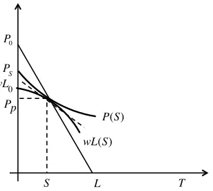
Let us analyze the intersection of two curves, the expenditures P(S) curve and the labor income
wL(S) curve, where T is the time horizon of the consumption-leisure choice (T = L + S +H), the value w×∂L/∂S is negative (w×∂L/∂S<0), because the best offer PP=wL exceeds the aspiration
level wL0 and the value ∂P/∂S, which is exposed at the moment of purchase by the tangent dotted
line, is also negative, now with regard to the assumption of the diminishing marginal efficiency of search (Figure 1):
S
wL
0
Pp
T
P(S) PS
[image:3.595.194.352.326.461.2]wL(S)
Figure 1. Reservation level, the starting price, and the purchase price
If the value PP is equal to the actual labor income wL(S) at the moment of purchase, the slope of
the wage rate (-w) gives us the value of the labor time L required for the purchase on horizontal axis. In addition, it also gives us the value P0 on the vertical axis, which is equal to the potential
labor income (Figure 2), or
P
0 =w(L+S) (1)
S
wL
0 Pp
T P(S)
P
S
P0
[image:4.595.195.349.60.198.2]L wL(S)
Figure 2. Actual vs. potential labor income
The Figure 2 shows that the absolute value of the decrease in the potential labor income at the moment of purchase is greater than the absolute value of the decrease in the actual labor income, or w >|w×∂L/∂S|. This consideration attracts attention to the core function L(S). Indeed, when we
take the values ∂P/∂S<0, ∂2P/∂S2>0 of the expenditures’ function P(S), we simply follow the
assumption of the diminishing marginal efficiency of search. However, the behavior of the L(S)
function is not so clear.
When the search S “squeezes out” the labor L and the leisure H from the given time horizon T, like ice displaces both whiskey and soda in the glass, the ∂L/∂S rate directly depends on the
value ∂H/∂S because ∂L/∂S+1+∂H/∂S=0. However, the value ∂H/∂S can be determined by a
very simple rule. If we take the differential dH(S), we can see that the absolute rate of the decrease in leisure time is equal to its share in the time horizon, or |∂H/∂S|=H/T and H/T= - ∂H/∂S. From here we can get the value of the propensity to search ∂L/∂S. It is negative because
the labor and the search represent alternative sources of income. We can also get the derivatives of propensity to search, which are very important for our analysis:
L(S)=T−H(S)−S;
∂L/∂S=−∂H/∂S−1;
dH(S)=dS∂H ∂S =−
dSH T
⇓
∂L ∂S =−
∂H ∂S −1=
H
T −1= H−T
T =− L+S
T (2.1)
∂L ∂S =
H−T
T ⇒ ∂ 2L
/∂S∂H=1 /T; (2.2)
∂L ∂S =−
L+S
T ⇒ ∂ 2L
/∂S2=−∂L/∂S+1
T <0 (2.3) 2
If at the moment of purchase the marginal loss in labor income is equal to the marginal benefit of the search, the Equation (2.1) gives us:
Q∂P ∂S =w
∂L ∂S =w
H−T T =−w
L+S
T (3)
If we re-arrange the Equations (1) and (3) for the value of consumption Q=1, we see that the value of potential labor income is equal to the value of the time horizon times the value of the price reduction at the moment of purchase (Figure 3), or
2
P
0=−T× ∂P/∂S=w(L+S) (4)
S wL
0 Pp
T P(S)
P S P0
[image:5.595.194.373.56.217.2]L wL(S)
Figure 3. Potential labor income, price reduction, and time horizon
3.Satisficing Marginal Decision: indirect proof
Now we can proceed to the indirect proof of the correspondence of the optimal search-stopping rule to the satisficing choice.
Let us take the “apple of discord” between psychologists and economists. We presuppose that at the moment of purchase the absolute value of the marginal decrease in the labor income for the given wage rate w is still less than the marginal benefit of the search, or:3
w∂L ∂S <
∂P
∂S (5)
It seems that the optimizing approach requires continuing the search while the satisficing decision has already stopped it. However, the Equation 4 tells us that this case should result in the hypothetical value P0’, where we comes to the following inequality for the given wage rate
w:
P
0'=w(L'+S')<P0 =w(L+S) (6)
Due to the rule ∂2L/∂S2<0 from the Equation (2.3), the inequality (L’+S’)<(L+S) produces the
following inequalities: L’ >L and S’ <S. And we can see that our assumption is false, because either the hypothetical amount of search S’ should be less than the actual amount of search S and the greater hypothetical amount of labor L’ results in a greater purchase price P’P >PP, or the
actual amount of search S should diminish the labor time required for the purchase and it should result in the value P’P <PP.
We can graphically confirm the last consideration, if we take the [P’0;L’] line, which also has the
(-w) slope (Figure 4):
S
wL 0
Pp
T P(S)
PS P0
L wL(S) P0
'
Pp!
S' L'
Figure 4.The indirect proof of the equality of the marginal values of search
3
[image:5.595.193.344.572.711.2]The same indirect proof can be applied when it is supposed that at the purchase price level the marginal costs of search are decreasing faster than its marginal benefit. The only difference is that this case can be eliminated from the analysis by definition, because it requires recognition that the chosen price is not satisficing. The satisficing cognitive mechanism stops working and the mechanism of discouragement takes place.4 Indeed, we can reproduce the set of inequalities, which describe the dissatisfying choice, when a high price corresponds to unexpectedly low savings on purchase and the loss in labor income is greater than savings on purchase:
w∂L
∂S > ∂P ∂S (7)
dS w∂L ∂S >dS
∂P
∂S (8)
dwL(S)>dP(S)
When the inequalities (5) and (7) are false, the Equation (3) takes place. Now we can say that
when the consumer chooses the satisficing price, his decision automatically equalizes the marginal loss in the labor income with the marginal benefit of the search.
This proof can be repeated for any pre-allocated quantity Q. There, the Equation (4) takes the following form:
QP0 = - T×Q×∂P/∂S = w×(L+S) (9) 5
The Figure 4 provides us with another interesting consideration. Let us pay attention to the situation when the same amount of search S results in a price P’P<<wL0, i.e., when the best
offer, an unexpected price discount, for example, significantly exceeds the aspiration level – the case that can really challenge the optimizing approach. Here we realize that the absolute value of the actual price reduction |∂P/∂S| is greater than its planned value |dP/dS|. It seems that if the
consumer accepts this price, he doesn’t equalize marginal costs of the search |w×∂L/∂S| with its
marginal benefit |∂P/∂S|.
However, this decision changes not only the value of the marginal benefit of the search but it also changes both the propensity to search and the marginal loss in the labor income. It happens because the choice of the lower price decreases, as Figure 4 shows and the Equation (1) proves it, the value T of the time horizon of the consumption-leisure choice.
The time horizon of the consumption-leisure choice, i.e., the time to the next purchase, depends on products’ lifecycles. The lower price can exhibit the coming expiration date for pork sausages, for example.
If we remember the famous metaphor of M.Friedman and L.J.Savage, when they compared economic agents with billiard players, who make their shots as if they know the complicated mathematical formulas, we should not forget that billiard is played by two people. The seller doesn’t bother about consumer’s marginal values of search, but either he cut the price for before-yesterday “fresh” sausages, or he offers packed pork sausages with extended shelf life. In addition, if the consumer buys before-yesterday “fresh” sausages, he should quickly eat them, i.e., to cut leisure time H, reserved for the consumption.
If the consumer doesn’t accept this lower price because he estimates it as too high price for the shorter shelf life, we meet again inequalities (7) and (8) of the dissatisfying choice. So, the
4
The description of the cognitive mechanisms was presented by H.Simon in the Psychological Review in 1967 (Simon 1967).
5
producer should support the shorter shelf life by the corresponding price discount |P’P - PP|
(Figure 5):
S
wL 0 Pp
T P'(S)
PS P0
L
wL'(S)
P0
'
Pp!
[image:7.595.193.349.92.235.2]L' T'
Figure 5. Price discount for the short shelf life
Now, the new search path P’(S) meets the decrease in the labor income wL’(S) at the point (S;P’P). The P’(S) curve becomes steeper due to the price discount and the wL’(S) curve
becomes steeper due to the shorten time horizon T’. So, for the same amount of the search S and for the labor income required for the purchase wL’<wL we have
∂P'
∂S = w∂L'
∂S =−
wL'+S
T' (10)
The time horizon T’ is cut here not only by the decrease in the labor time L but also by the decrease in time of consumption, i.e., leisure time H, or ΔT=ΔL+ΔH. So, the absolute value of
the propensity to search |∂L/∂S| becomes greater. In addition, the [P’0;T’] line also becomes
steeper than the initial [P0;T] line because the absolute value of the equilibrium price reduction
|∂P/∂S| becomes greater.6
This example provides us with the deeper understanding of the phenomenon of the visual disparity between the satisficing approach and the optimizing model. Let us come back to the “apple of discord”, i.e., to the inequality of marginal values of search, or |w×∂L/∂S|<|∂P/∂S| and,
as a result, to the inequality w(L +S)<P0.
If we analyze the value of propensity to search ∂L/∂S, we can see that its absolute value |∂L/∂S|
can be raised to the level of the equality with the absolute value of price reduction |∂P/∂S | in two
ways. One way is to search more intensively and to increase the (L + S) value with the help of the ∂2L/∂S2<0 rate. But there is another way. If the individual cuts the time horizon T, he also
increases the absolute value of the marginal costs of search |w×∂L/∂S|. Why the decrease in the
time horizon happens here?
Let us imagine two low-wage rate individuals who enter the high-price suit store. The first visitor does not accept high prices while the second visitor makes the purchase. We understand that they have different reservation prices. The first consumer decides either to search for a lower price or to wait for sales. And the second consumer is more impatient. He accepts the high price, which is satisficing for him. His impatience increases the reservation level and it also hastens the moment of consumption. Moreover, the impatience intensifies the consumption. When the first visitor finally buys the chosen suit at a lower price at sales he will put it on occasionally. However, when the impatient consumer buys the high-price suit he will often wear it because he likes it more than his friend.
We can check all these considerations by the Equation (3). We suppose that both visitors have the same potential labor income w(L +S). (This assumption will be validated in Part 4.) But they have different time horizons because they have either different intensity of consumption Q/H
and/or different attitudes to fashion products. The first consumer can wait for sales while the
6
second cannot. On the other hand, when the impatient consumer intends to wear new fashion suit often and in current season, he decreases both the total time of its consumption, i.e., the leisure time, and the time horizon. Evidently, in this case the suit either becomes shabby soon or it goes out of vogue. But the decrease in the time horizon increases the absolute value of the marginal costs of search |w×∂L/∂S|. And this new value of |w×∂L/∂S| meets the high value of the price
reduction |∂P/∂S|:7
P
0=w(L+S)=−T1× ∂P1/∂S1=−T2× ∂P2 /∂S2;
T
1>T2⇒|∂P1/∂S1|<|∂P2/∂S2| (11)
The high price becomes satisficing for the impatient consumer while it stays above the reservation level of the first consumer.
This example shows how the fashion can increase the reservation level and at the same time it can cut the “shelf life” of the chosen item. However, there are markets where all consumers are impatient as well as intensive in consumption. The fish market represents a good example of this kind of the total impatience.
4.Optimization of Satisficing Decision
The model presented here describes the sequential search as the passage from one value of marginal savings |∂P/∂S| to the other |∂P/∂S| value with a predetermined consumption Q. In this
sense the sequential search is a dynamic process. However, this consideration also gives us the orthogonal view. We can solve the optimization problem for a static |∂P/∂S| value.
It seems that the optimization of the utility function U=U(Q,H) is not possible here due to the predetermined value of Q and respectively due to the value ∂Q/∂H=0. However, the really static
methodology overrides this problem. We can come back to H.Leibenstein’s definition of “of a static situation as one in which the order of events is of no significance”. (Leibenstein, 1950, p.187). And we can take either a consumer who stops the search at a certain |∂P/∂S| value and
who decides after that how much he should consume for the given time horizon, a week, for example, and how much he should work in order to buy the chosen quantity, or a consumer who implicitly makes the consumption-leisure trade-off before he enters the particular market. In these both senses, the derivative ∂Q/∂H really takes place because the consumption-leisure
trade-off takes place.
T H*
U(Q,H) w∂L/∂S
∂P/∂S=Q *
L+S H
Q
− w ∂P/∂S
Figure 6. Satisficing optimal consumer choice
7
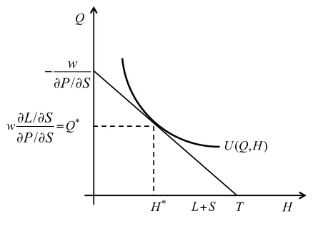
Let us suppose that a consumer has no liquidity constraint, for example, due to his strong precautionary motive (Carroll 2001, Malakhov 2011). Then, we can solve the static optimization problem of his consumption-leisure choice not with regard to the liquidity constraint but with regard to the equality of the marginal values of search, where the utility function has the common Cobb-Douglas form U(Q,H) = Q-∂L/∂SH-∂H/∂S =Q(L+S)/THH/T and the budget constraint line connects the time horizon T with the corner solution for leisure (H=0;∂L/∂S=-1) (Figure 6).
As a result, we have the following Lagrangian equation:8
Λ=U(Q,H)+λ(w−Q∂P/∂S ∂L/∂S) (12)
If we take the value ∂P/∂S as the value given by a particular local market, either by a
convenient store or a supermarket, we can solve the optimization problem U(Q,H) of the consumption-leisure choice with regard to this particular market, keeping in mind the derivative of the propensity to search from the Equation (2.2):
∂U
∂Q =λ
∂P/∂S
∂L/∂S;
∂U
∂H =−λw
∂2
L/∂S∂H
∂L/∂S ;
∂U/∂H
∂U/∂Q=MRS(HforQ)=−
w
∂P/∂S∂
2
L/∂S∂H=− w
T× ∂P/∂S = w
P0 (13)
The marginal rate of substitution of leisure for consumption MRS (H for Q) is determined here not by the purchase price like in the classical model of the individual labor supply but by the price equivalent of the potential labor income. The Equation (13) tells us that the value of potential labor income corresponds to the equilibrium price. Indeed, while the monetary loss during the search is equal to the value dS×w×∂L/∂S, the costs of search or transaction costs are
equal to the value w×dS. So, the equilibrium price is equal to the sum of labor costs and
transaction costs. If we come back to two friends regarding the fashion suit, we can see that although they have different reservation prices, the equilibrium price is unique and it is equal to their potential labor income.
The graphic illustration of the optimization problem shows that the marginal rate of substitution is equal to the common microeconomics ratio of consumption to non-leisure time, or
MRS(H for Q)=−∂Q
∂H =
Q*
L+S =
w
P0 (14)
However, when we combine this result with the Equation (13), we get another confirmation of the Equation (9) and another illustration for the equilibrium price:
MRS(HforQ)=−∂Q
∂H =
Q* L+S =
w P0;
w(L+S)=Q*
P0 (15)
5.Application of Satisficing Optimal Decision: Paradox of Little Pre-Purchase Search for Big-Ticket Items
Our analysis discovers the general relationship between marginal savings on purchases ∂P/∂S,
the time horizon of the consumption-leisure choice, and the potential labor income:
−∂P ∂S =
P
0
T (16)
This relationship can be illustrated by the paradox of little pre-purchase search for big-ticket items. In 1979 Kapteyn et al. published the results of the survey on consumer behavior. The
8
author found that purchase decision concerned durables had been satisficing rather than maximizing (Kapteyn et al. 1979). Later Grewal and Marmorstein made the following comment to those results:
“Previous studies have consistently found that most consumers undertake relatively little pre-purchase search for durable goods and do even less price-comparison shopping,.. (when) prices of the more expensive products tend to exhibit the greatest variation across stores. Given the aforementioned evidence regarding the price variation of big-ticket items, it appears that many consumers engage in considerably less price search than is predicted by the economics-of-information theory.” (Grewal and Marmorstein 1994, p.453)
R.Thaler documented that anomaly in the following manner:
“One application of marginal analysis is optimal search. Search for the lowest price should continue until the expected marginal gain equals the value of the search costs. This is likely to be violated if the context of the search influences the perception of the value of the savings. In Thaler (1980), I argued that individuals were more likely to spend 20 minutes to save $5 on the purchase of a $25 clock radio than to save the same amount on the purchase of a $500 television.” (Thaler 1987, pp.110-111)
We can check the results of R.Thaler’s experiment in order to show that there was no anomaly and that the case did not conflict with the marginal approach.
Suppose an individual who is ready to give up 20 hours of leisure to get (i.e., to work and to search for) a big-ticket item Qbti and only 1 hour of leisure to get a cheap item Qci. If we take the
value dP as the constant, “the same amount” in R.Thaler’s experiment, for both items and, when
S0=0 and S=dS, we have:
∂P
∂S =
w∂L
∂S =−
wL+S
T ;
dP(S)=dS∂P
∂S =−
wL+S
T dS;
dP(S)
=
−wLbti+SbtiT dS
bti=−w
L
ci+Sci
T dS
ci; (17)
dP(S)=−w20 T
dS
bti=−w 1
T dS
ci;
20S
bti=Sci
When the individual finally makes these both purchases, he realizes that he has spent twenty times more on the search for the cheap item than on the search for the big-ticket item. The advice of “a reliable friend” to go to the other shop for $5 discount in R.Thaler’s experiment could not give more than a minute to exit from the shop, to enter into another shop, and to buy there the $500 TV with $5 discount.
6.Conclusion
The analysis of the paradox of little pre-purchase search for big-ticket items follows the general idea of the paper – economic agents are more rational in everyday life that it is usually considered. The observed anomalies of economic behavior don’t illustrate irrationality but they need deeper economic understanding, which could reinforce the predictive power of economic considerations.
The application of the optimization rule to the satisficing consumer decision simply represents the illustration of Friedman-Savage billiard metaphor. Here, the billiard shot corresponds to the explicit satisficing procedure, while the physical trajectory of a ball corresponds to the implicit optimization rule. Hence, the lucky shot shows how a psychological satisficing decision results in a natural optimal outcome.
not equal to the purchase price. However, the value of potential labor income could be hardly esteemed as a monopoly price. If a monopoly sets its price at the level of potential labor income, workers should substitute search by labor. As a result, the labor market decreases the wage rate in response to this additional labor supply and the monopoly price becomes unattainable.
The model proposes another methodological explanation of the difference between a purchase price and an equilibrium price. The search produces the monetary loss in labor income with regard to the reservation price or to the willingness to pay (WTP=wL0). Here, the value of
|w×∂L/∂S| is equal to the marginal loss in labor income in the explicit monetary model and to the
marginal value of leisure in the implicit model of utility. 9 However, if a consumer decides to sell an item after the purchase he takes into account not the monetary loss but the costs of search, which should be total but not marginal. Therefore, he takes into account the wage rate and the time of search, or to the value wS. And here we come to consumer’s willingness to accept (WTA). This consideration results in the assumption that when search costs are positive the equilibrium price is equal to the willingness to accept. This assumption becomes more plausible if we consider home production to be a specific form of search, where the purchase price is equal to the price of inputs and the equilibrium price or the willingness to accept is equal to the sum of the price of inputs wL and the transformation costs wS.
The correspondence of the equilibrium price to the willingness to accept could explain the WTP-WTA disparity documented in many studies (see, for example, Horowitz et al. 2003). However, if we find the satisficing price at the beginning of the search (i.e., S=0) and the WTP-WTA disparity disappears. The utility function takes the following form U(Q,H)= Q-∂L/∂SH-∂H/∂S =QL/THH/T , the values of equilibrium marginal utilities of both consumption and leisure become equal to the corresponding values in the classical model of individual labor supply, and the Hicksian WTP-WTA equivalence takes place. In addition, the potential labor income, i.e, the equilibrium price, becomes equal to the purchase price. The market becomes perfect.
References
1.Aguiar M., Hurst E. (2007). Lifecycle Prices and Production. American Economic Review. 97(5). 1533-59. http://dx.doi.org/10.1257/aer.97.5.1533
2.Carroll, C.D. (2001). A Theory of the Consumption Function, with and without Liquidity Constraints. Journal of Economic Perspectives. 15(3). 23-45.
http://dx.doi.org/10.1257/jep.15.3.23
3.Cesario, F. J. (1976) Value of Time in Recreation Benefit Studies. Land Economics. 52(1). 32-41. http://dx.doi.org/10.2307/3144984
4.Diamond, P. (1971). A Model of Price Adjustment. Journal of Economic Theory. 3. 156-168. http://dx.doi.org/10.1016/0022-0531(71)90013-5
5.Fellner, G., Guth,W., Martin E. (2006). Satisficing or Optimizing? An Experimental Study. Max-Planck-Institut für Ökonomik. Papers on Strategic Interaction. 11.
9
http://www.researchgate.net/publication/5018160_Satisficing_or_Optimizing_-_An_Experimental_Study
6.Friedman, M. (1953). Essays in Positive Economics. Part I. The Methodology of Positive Economics. University of Chicago Press (1953) 1970.
7.Grewal D., Marmorstein, H. (1994). Market Price Variation, Perceived Price Variation, and Consumers’ Price Search Decisions for Durable Goods. Journal of Consumer Research. 21 (3). 453-460. http://dx.doi.org/10.1086/209410
8.Horowitz, J. K., McConnell, K. E. (2003). Willingness to accept, willingness to pay and the income effect. Journal of Economic Behavior & Organization. 51(4). 537-545
http://dx.doi.org/10.1016/S0167-2681(02)00216-0
9.Kapteyn A., Wansbeek T., Buyze J. (1979). Maximizing or Satisficing. The Review of Economics and Statistics. 61 (4). 549-563. http://dx.doi.org/10.2307/1935786
10.Larsons,D.M., Shaikh S.(2004). Recreation Demand Choices and Revealed Values of Leisure Time. Economic Inquiry. 42 (2),264-278.
http://home.uchicago.edu/~sabina/Economic%20Inquiry.pdf
11.Leibenstein, H. (1950). Bandwagon, snob, and Veblen Effects in the theory of consumers' demand. Quarterly Journal of Economics. 64. 183-207.http://dx.doi.org/10.2307/1882692
12.Lewer, J., Gerlich, N., Gretz, R. (2009). Maximizing and Satisficing Consumer Behavior: Model and Test. Southwestern Economic Review (Texas Christian University). 36 (1). http://ssrn.com/abstract=1740002
13.Malakhov, S. (2011). Optimal Consumer Choices under Conditions of Sequential Search.(in Russian) Economic Policy. 6 (6) 148 - 168. The English version is availaible as “Optimal Sequential Search and Optimal Consumption-Leisure Choice” at:
http://works.bepress.com/sergey_malakhov
14.Malakhov, S. (2013). Money Flexibility and Optimal Consumption-Leisure Choice
Theoretical and Practical Research in Economic Fields. IV(1).77-88. http://asers.eu/asers_files/tpref/TPREF%20Volume%20IV%20Issue%201_7_%20Summer% 202013_last.pdf
15.Malakhov, S. (2014). Sunk Costs of Consumer Search: Economic Rationality of Satisficing Decision. Forthcoming in Theoretical and Practical Research in Economic Fields. 5. 1(9), available at http://works.bepress.com/sergey_malakhov
16.Simon, H. (1957). Part IV in: Models of Man. Wiley, New York, 196 – 279.
18.Simon, H. (1972). Theories of Bounded Rationality. In C.B.Mcguire and Roy Radner (eds.)
Decision and Organization. Nort-Holland Publishing Company, 161 – 176.
19.Simon, H. (1978). Rationality as Process and as Product of Thought. American Economic Review. 68(2). 1-16.
20.Slote, M. (1989). Beyond Optimizing: a study of rational choice. Harvard University Press. http://dx.doi.org/10.4159/harvard.9780674434417
21.Schwartz, B., Ward, A., Monterosso, J., Lyubomirsky, S., White, K., Lehman, D. (2002). Maximizing Versus Satisficing: Happiness is a Matter of Choice. Journal of Personality and Social Psychology. 83 (5). 1178-1197.
http://psycnet.apa.org/psycinfo/2002-18731-012
22.Thaler, R. (1980). Toward a Positive Theory of Consumer Choice. Journal of Economic Behavior and Organization. 1. 39-60. http://dx.doi.org/10.1016/0167-2681(80)90051-7