Is the Chinese Stock Market Really Efficient

(1)

Munich Personal RePEc Archive

Is the Chinese Stock Market Really

Efficient

Yan, Isabel K. and Chong, Terence and Lam, Tau-Hing

City University of Hong Kong, Chinese University of Hong Kong

August 2011

Online at

https://mpra.ub.uni-muenchen.de/35219/

(2)

1

Is the Chinese Stock Market Really Inefficient?

Terence Tai-Leung Chong1

Department of Economics and Institute of Global Economics and Finance The Chinese University of Hong Kong

Tau-Hing Lam Department of Economics The Chinese University of Hong Kong

Isabel Kit-Ming Yan

Department of Economics and Finance City University of Hong Kong

August 14, 2011

Abstract

Groenewold et al (2004a) documented that the Chinese stock market is inefficient. In this

paper, we revisit the efficiency problem of the Chinese stock market using time-series

model based trading rules. Our paper distinguishes itself from previous studies in several

aspects. First, while previous studies concentrate on the viability of linear forecasting

techniques, we evaluate the profitability of the forecasts of the self-exciting threshold

autoregressive model (SETAR), and compare it with the conventional linear AR and MA

trading rules. Second, the finding of market inefficiency in earlier studies mainly rest on

the statistical significance of the autocorrelation or regression coefficients. In contrast,

this paper directly examines the profitability of various trading rules. Third, our sample

covers an extensive period of 1991-2010. Sub-sample analysis shows that positive returns

mainly concentrate in the pre-SOE reform period, suggesting that China’s stock market

has become more efficient after the reform.

Keywords: Efficient Market Hypothesis; SETAR Model; Bootstrapping; SOE reform.

JEL Classifications: C22, G10, G12.

1

(3)

2

1. Introduction

Given the rising importance of the Chinese stock market, it is natural to ask whether

profitable trading strategies exist in the Chinese stock exchanges. If one can predict

returns consistently using past information, we would have a violation of the efficient

market hypothesis (EMH). However, the issue of stock market efficiency is probably one

of the areas with the largest discord between academic literature and public media. While

technical analysis is widely used by investors to formulate trading strategies, the concept

of stock market efficiency in the academic literature suggests that current asset prices

should fully reflect all past information at any point of time and hence no market players

should be able to profit from using technical trading rules.

A series of studies have contributed to this debate in the past. Studies that provide

supporting evidence for the EMH include Bailey (1994), Cai et al. (1997), Liu et al.

(1997), Long et al. (1999), Xu (2000), Darrat and Zhong (2000) and Chen and Li (2006).

Studies that present counter evidence include Su and Fleisher (1998), Abdel-Khalik et al.

(1999), Chow et al. (1999), Mookerjee and Yu (1999), Ma (2000), Kang, et al. (2002),

Groenewold et al. (2004a), Chen and Li (2006), Balsara et al. (2007) and Chen et al.

(2010).

Some explanations have been offered in the literature for the ambiguity in the findings of

different studies. For example, Groenewold et al. (2004a) point out that the difference can

be attributed to the properties of the sample periods used in various studies. Xu (2000),

for instance, reports the absence of significant autocorrelations in the Shanghai

Composite Index after omitting the early turbulent years of Mookerjee and Yu (1999)’s

sample and extending the sample to 1995. The effects of reforms are also found to play

an important role. Groenewold et al. (2003) find that the efficiency of the stock market

tends to improve after the banks were re-admitted in 20002. Another study by Wang et al.

(2009) investigates the change of weak form efficiency brought by reform on the range of

2

(4)

3

price variations. Using rolling window estimation on the daily closing price of the

Shenzhen Component Index during 3 April 1991 and 15 December 2008, they conclude

that the reform improved market efficiency substantially in the long run but the influence

in the short run is small.

In this paper, we revisit the efficiency problem of the Chinese stock market by examining

the profitability of trading rules based on time series models. Following Chong and Lam

(2010), we study the performance of the self-exciting threshold autoregressive (SETAR)

model, the autoregressive (AR) model and the moving average (MA) model in generating

profitable trading rules for the Composite Indices of the Chinese stock market. Our paper

distinguishes itself from previous studies in four aspects. First, while previous studies

concentrate on the viability of linear forecasting techniques, we evaluate the profitability

of the SETAR forecast, and compare it with the conventional linear AR and MA trading

rules.3

Second, the studies cited earlier generally apply efficiency tests (like autocorrelation

coefficient tests, run tests and variance ratio tests) or linear regressions (like VAR and

ARIMA models) in their analysis. Their conclusion on inefficiency mainly rests on the

statistical significance of the autocorrelation coefficients or regression coefficients but

not on the actual profitability of the predictive models. This paper provides an alternative

to the standard EMH tests and address the question of whether the predictability found in

weak EMH tests implies profitability.

Third, previous studies on the Chinese Stock market focus on the A and B share indices

(Cai et al., 2005; Tian et al., 2002). In this paper, we focus on the Shanghai Composite

Index and the Shenzhen Composite Index, which have received relatively little attention

3

(5)

4

in the literature. To avert the data snooping problem (Sullivan et al., 1999), eleven

different trading rules are applied to the two composite indices.

Fourth, with the exception of Balsara et al. (2007) and Chen et al. (2010), all other studies

cited earlier only use data before 2002 and hence do not cover the period after major

reforms like the SOE reform. Balsara et al. (2007) and Chen et al. (2010) use data up to

2005 and 2006 respectively, but still do not go much beyond the time after the SOE

reform. In contrast, this paper employs data over an extensive sample period of

1991-2010. The longer sample provides us with a greater variety of information and should

reflect the dramatic changes that have taken place in China’s securities sector in the past

decades. It also sheds light on whether the results on EMH are sensitive to the

sub-periods used.

The rest of this paper is organized as follows. Section 2 describes the data. Section 3

presents the models and trading strategies. Section 4 discusses the empirical results.

Section 5 conducts a bootstrap analysis, and Section 6 concludes the paper.

2. Data

2.1. Institutional Background

The Chinese stock market has a relatively short history, with the Shanghai and Shenzhen

Stock Exchanges launched only in the early 1990s. The Shanghai Stock Exchange was

established on November 26, 1990, while the Shenzhen Stock Exchanges was opened on

April 11, 1991. Two categories of shares are traded in the Chinese market, namely, the A

shares and the B shares. The A-share market and the B-share market are segmented.

Tradable A-shares are available exclusively for domestic citizens and institutions, while

(6)

5

domestic investors in February 2001.4 Both the stock exchanges in Shanghai and

Shenzhen have experienced phenomenal growth since their inception. At the outset of

2011, there were already 901 listed companies in the Shanghai Stock Exchange (SHSE)

with a total market capitalization of about 18238 billion RMB, and 1202 listed companies

in the Shenzhen Stock Exchange (SZSE) with a total market capitalization of 8416 billion

RMB. The combined Chinese stock market rivals the Hong Kong Stock Exchange as

Asia’s second-largest stock market after the Tokyo Stock Exchange.

2.2. Shanghai Composite Index and Shenzhen Composite Index

Both the Shanghai Composite (SHC) Index and the Shenzhen Composite (SZC) Index are

examined in this paper. The constituents of the Shanghai Composite (SHC) Index are all

stocks (A shares and B shares) listed in the Shanghai Stock Exchange. The base day for

the SHC index is December 19, 1990, and the base value is 100. The index was officially

launched on July 15, 1991.5 The Shenzhen Composite (SZC) Index is a

market-capitalization weighted index of stocks in the Shenzhen Stock Exchange which tracks the

daily price movements of all the shares in the exchange. The index began on April 3,

1991, with a base price of 100. The sample contains 4808 daily observations from the

SHC (Jan 1991 to Aug 2010) and 4717 daily observations from the SZC (April 1991 to

Aug 2010) taken from DataStream.

In the first decade of the establishment of the two stock exchanges, most of the listed

firms in China were restructured SOEs. In April 2005, the China Securities Regulatory

Commission launched a state share reform, aiming at converting the non-tradable state

shares to tradable shares. As part of the SOE reform, shares of a typical firm are split into

state shares, legal-entity shares and tradable shares.6 Since the reform, the market has

undergone another phase of rapid development. During 2005 to 2007, the market indices

4

Before 2001, only foreigners or foreign institutions were allowed to trade B Shares. From February 2001 onwards, local investors are also permitted to trade B Shares via legal foreign currency accounts.

5

The B shares are generally denominated in US dollars for calculation purposes. For calculation of other indices, B share stock prices are converted to RMB at the applicable exchange rate (the middle price of US dollar on the last trading day of each week) at China Foreign Exchange Trading Center.

6

(7)

6

kept soaring. The stock market capitalization in China surpassed its GDP, and the number

of investors has burgeoned to over 0.1 billion.

In view of the structural changes, we divide the whole series into four subsamples at the

criterion of the date of the SOE reform and the recent financial crisis. The first

sub-sample starts at the beginning of the sub-sample to the end of March 2005, which represents

the stage before the SOE reform. Before April 2005, companies listed on the Chinese

stock market had a split-share structure with roughly 1/3 freely traded public stocks (TS)

and 2/3 nontradable state-owned shares (NTS). The second sub-sample covers the period

from April 2005 to Nov 30 2006. In April 2005, the China Securities Regulatory

Commission launched a state share reform, aiming at converting the NTS state to TS.

According to the latest report in Nov 2006, 90% of Chinese firms had complied with the

orders to reform their share structure7. The third sub-sample starts with the onset of the

recent financial crisis at the end of 2006 and lasts until the end of March 2009 which

marks the trough of the crisis. This sub-sample is characterized by market panic and

extreme volatility. The last sub-sample covers the period after the trough of the financial

crisis. It extends from April 2009 to the end of the whole sample in Aug 2010.8 Table 1

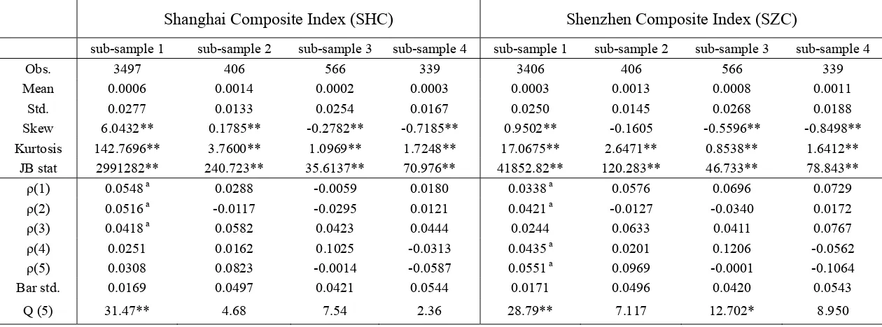
provides the summary statistics of the one-day returns in the sub-samples.

INSERT TABLE 1 Here

Returns are calculated as the log difference of the stock index level. “JB stat” represents

the Jarque-Bera test for normality. ρ(i) refers to the estimated autocorrelation at lag i. Q(5)

denotes the Ljung-Box Q statistics at lag 5. “Bar std.” refers to the Bartlett asymptotic

standard error band for autocorrelations. Autocorrelations marked with (a) are greater

than twice the Bartlett asymptotic standard error band. Numbers marked with * and **

are significant at the 5% and 1% level respectively. From the values of the skewness,

kurtosis and Jarque-Bera (JB) statistics, it is found that the returns are leptokurtic, skewed

and non-normal. We further calculate the autocorrelations and the Ljung-Box Q statistics.

7

Huang et al. (2008) provide more details of the reform.

8

(8)

7

For the Shanghai Composite Index (SHC), the Ljung-Box Q statistic at the fifth lag is

statistically significant only in the first sub-sample prior to the SOE reform, which

suggests the presence of autocorrelation in this period. For the Shenzhen Composite

Index (SZC), the Ljung-Box Q statistic is significant at the 1% level in the first

sub-sample and at the 5% level in the third sub-sub-sample during the financial crisis. No

significant autocorrelation is evident in the other sub-samples.

3. Trading Strategies

Voluminous studies in the literature have examined the usefulness of technical trading

rules in generating abnormal profits. Some popular technical trading strategies in use

today include those based on supports and resistances, filter rules, moving averages and

relative strengths. Previous studies, including those of Fama (1965, 1970) and Jensen and

Benington (1970), find that historical prices cannot be used to predict future prices.

Similarly, Hudson et al. (1996) demonstrate that the moving averages (MA) and trading

range breakout (TRB) rules cannot beat the buy-and-hold strategy in a costly trading

environment. Allen and Karjalainen (1999) also argue that technical rules cannot

outperform the buy-and-hold strategy. Coutts and Cheung (2000) investigate the

profitability of the MA and TRB trading rules in the Hong Kong stock market and show

that they fail to generate abnormal returns. In contrast, Ferguson and Treynor (1985) find

that when nonprice information is taken into consideration, technical trading rules can

yield abnormal returns. Brock et al. (1992) and Bessembinder and Chan (1995) show that

the MA and TRB rules outpace the buy-and-hold strategy for the Dow Jones Industrial

Average. Mills (1997) obtain a similar result for the FT30 index. Chong and Lam (2010)

show that nonlinear trading rules are profitable in the U.S. stock market.

Most of the aforementioned studies focus on developed markets. Recently, there has been

a growing interest in the performance of technical trading rules in emerging markets.

Bessembinder and Chan (1995) conclude that the technical trading strategies are

(9)

8

and Gunasekarage and Power (2001) also report significant trading-rule profits in the

Latin American and South Asian stock markets. More recently, Chong and Ip (2009) find

that momentum trading rules generate impressive returns in emerging currency markets.

In this section, we study the performance of the self-exciting threshold autoregressive

(SETAR) model, the autoregressive (AR) model and the moving average (MA) model in

generating profitable trading rules for the Composite Indices of the Chinese stock market.

3.1 Self-exciting Threshold Autoregressive (SETAR) Model

The following self-exciting threshold autoregressive model (Tong, 1978; Chong et al.,

2008) is estimated for the stock-index returns:



0 1 1









0 1 1







t t t d t t d t

Y   Y_ I Y_    Y_ I Y_  

            , (1)

where Yt denotes the natural logarithm of the stock index at day t, ΔYt is the continuously

compounded return on day t, d is the lagged parameter, and γ is the threshold value. I

 

A

is an indicator function which equals one if condition A is satisfied, and equals zero

otherwise.9 The error term is assumed to be a white noise.

The SETAR trading strategy is as follows:

B u y i f Yˆ_tw_₁> 0 , ( 2 )

S e l l i f w t

Yˆ_₁

 < 0 , ( 3 )

where w stands for the length of the observation window and Yˆ_tw_₁ refers to the predicted

9

(10)

9

return that is based upon information from the most recent w observations. In short, if the

predicted price of the next trading day is higher than the price of today, we buy the

Composite Index, otherwise we sell it.

3.2 Autoregressive and Moving Average Rules

The AR(1) model is a special case of SETAR(1) model. It can be written as:

0 1 1

t t t

Y   Y_ 

     . ( 4 )

Similar to the SETAR trading rule, we employ the recursive technique and define the AR

trading strategy as follows:

B u y i f w t

Yˆ_₁

 > 0 , ( 5 )

S e l l i f Yˆ_tw_₁< 0 , ( 6 )

If the predicted price of the next trading day is higher than the price today, we buy the

Composite Index, otherwise we sell it.

The moving average method has also been widely studied. A moving average with a

window size of w is defined as:

MAt(w)=(Pt+Pt-1+…+Pt-w+1 )/w, (7)

where Pt is the stock price at day t.

The trading rule is as follows:

B u y i f MA S_t( )MA L_t( ) , ( 7 )

(11)

10

where MA S_t( ) and MA L_t( ) represent the short-term MA and the long-term MA

respectively. If the short-term moving average is higher than the long-term moving

average, we hold a long the Composite Index. Otherwise, we hold a short position.

4. Empirical Results

On each trading day, a position of buy, sell, or neutral is taken based on the trading

signals. The one-day conditional mean and variance of buy (sell) returns can be written as

follows:

( )

( ) 1

1 ( ) 1 N

b s

b s t t

t b s Y I N  _ 





 ( 9 )

and

2 2 ( )

( ) 1 ( )

1 ( ) 1 ( ) N b s

b s t b s t

t b s Y I N  _  





  , ( 1 0 )

where _{b s}_{( )} stands for the mean return of the buy (sell) periods, _{b s}2_{( )} refers to the

conditional variance of the buy (sell) signals, N_{b s}_{( )} denotes the number of buy (sell) days,

N represents the number of observations, Y_t_₁ refers to the one-day holding period

return, and I_tb s( ) is an indicator function which equals one if a buy (sell) signal is

observed at time t, and zero otherwise. Following Brock et al. (1992), the null and

alternative hypotheses and the conventional t-ratio for the mean buy (sell) return are

given respectively as follows:

0: b s( )

H    ( 1 1 )

1: b s( )

H   ( 1 2 )

(12)

11 ( )

1

( ) ₂

2 2 ( ) b s b s b s t N N               

, ( 1 3 )

where  is the unconditional one-day mean and 2 is the unconditional variance.

The trading rules are evaluated by comparing the average returns for the buy and sell

periods. A good trading rule should be one for which the returns during buy periods

significantly exceed returns during sell periods. The following analysis tests for the

equality of means between the returns of the buy period and the sell period. The null and

alternative hypotheses and the t-statistic on the buy-sell spread can be expressed

respectively as follows:

0: b s 0

H    ( 1 4 )

1: b s 0

H    ( 1 5 )

and

1

( ) ₂ ₂ ₂

b s b s b s t N N              

. ( 1 6 )

The SETAR and AR models are estimated by the OLS method. The maximum lag is set

to five. We select the threshold and the lagged values by minimizing the residual sum of

squares. The numbers in parentheses are t-statistics testing whether the estimates are

statistically different from zero. “P-value” refers to the bootstrap p-value based on 500

simulations for testing the null hypothesis of no threshold effect10. The bootstrap

procedure is similar to that of Hansen (1997) under the assumption of homoscedastic

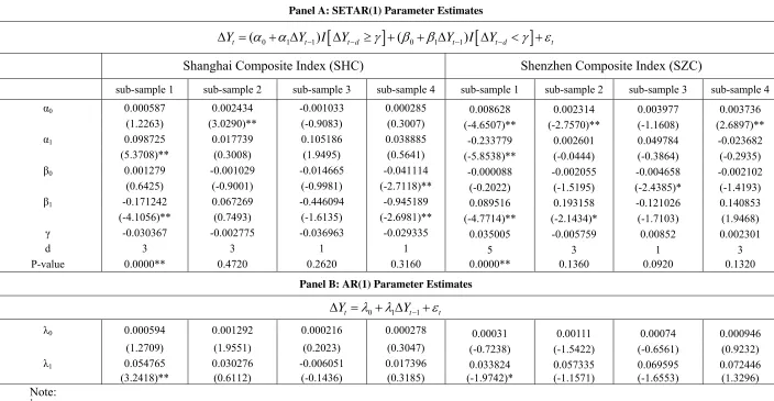
errors. Panel A of Table 2 contains the estimation results of Equation (1) using different

sub-samples. It is worthwhile noting that, during the first sub-sample --- the period before

the SOE reform, the AR coefficients are significant at the 1% level in both regimes and

10

(13)

12

evidence of threshold effect is found in both composite indices. The predictability in

terms of threshold effect and serial correlation is much weaker in the sub-samples after

the SOE reform. Some degree of serial correlation is evident in the Shanghai Composite

Index in the regime with selling signals (I



Y_t_₁ 0.029335



) during the post-crisis period (the 4th sub-sample) but not in the other regime. Panel B of Table 2 provides the

estimation results of the linear AR(1) model. Again, the AR coefficient is significant only

in the first sub-sample but not in the other sub-samples. This is consistent with increasing

efficiency in the market.

INSERT TABLE 2

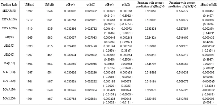
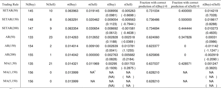
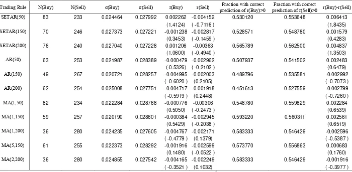
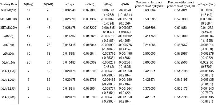
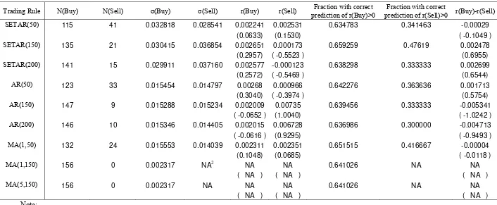
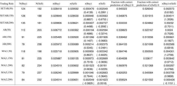
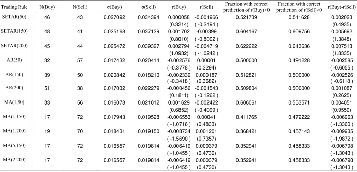
Tables 3a and 3b report the profitability of various trading rules.

INSERT TABLE 3a(i)-3a(iv) INSERT TABLE 3b(i)-3b(iv)

The trading period starts from day 250 onwards. The SETAR and the AR rules are

denoted by SETAR(w) and AR(w) respectively, where w represents the length of the

observation window. The MA rules are denoted as MA(S,L), where S refers to the

short-term MA and L refers to the long-short-term MA. The rules under study are MA(1,50),

MA(1,150), MA(1,200), MA(5,150) and MA(2,200). Columns 2 and 3 labeled “N(Buy)”

and “N(Sell)” report the number of buy and sell signals respectively. Columns 6, 7 and 10

show the one-day conditional mean for buy, sell and buy-sell returns respectively.

Columns 8 and 9 are, respectively, the fractions of buy and sell signals that produce

correct positive returns. The numbers in parentheses are the t-statistics for testing the null

hypotheses of (12) and (15). For the SHC sample, the returns are reported in Table 3a.

Our results suggest that most rules fail to produce significant returns, except for the

SETAR(200) and MA(1,50) models during the pre-SOE reform period (1st sub-sample).

These two models generate a buy-sell difference in returns of 0.2154% and 0.2211%

respectively in the Shanghai Stock Exchange sample. Nevertheless, such returns can

(14)

13

percent11, it will be difficult for investors to profit from these trading strategies.

5. Bootstrap Analysis

As the conventional t-test assumes a normal, stationary and independent error distribution,

the test results will be biased if the error terms are leptokurtic, serially correlated or

conditional heteroskedastic. In this section, we adopt the bootstrap method of Efron

(1979) to evaluate the significance of the trading-rule returns. The bootstrap technique

simulates the empirical distributions of the trading-rule returns under various null models

and hence provides critical values for gauging the significance of the trading-rule returns.

The null models examined in this paper include a random walk model with a drift and a

GARCH-M model. The bootstrap procedure consists of several steps. First, the null

model is estimated using the actual data and the residuals are obtained. Second, residuals

are drawn with replacement to generate the bootstrap return series using the estimated

coefficients of the null model. Third, the buy-returns and sell-returns using the bootstrap

sample under various trading rules are calculated. The mean, the standard deviation and

the t-statistics of various trading rules are then recorded accordingly. The procedure is

replicated 500 times (Efron and Tibshirani, 1986). The proportion of simulation results

which is larger than those from the actual series is the bootstrap p-value. We reject the

null hypothesis of zero buy-sell spreads at the 5 percent significance level if the buy-sell

returns derived from the actual series are larger than the 5 percent cutoff points of the

artificial buy-sell spreads generated from null models. In this study, stock prices are

simulated from two commonly used time series models. The first model is the

random-walk model with a drift:

constant

t t

Y 

   . ( 1 7 )

The random-walk specification is consistent with the EMH, which suggests that stock

11

(15)

14

prices are not predictable. As a result, the random-walk simulations allow us to construct

the confidence intervals for trading-rule returns under the null hypothesis.

The second model is the generalized autoregressive conditional heteroskedasticity in

mean (GARCH-M) model, which can be written as:

0 1 1 2

t t t t

Y   _  h 

     , ( 1 8 )

1

2

0 1 t 2 1

t t

h    _  h_ , ( 1 9 )

t

t h zt

  , ( 2 0 )

wherez_t ~N(0,1) and h_t refers to the conditional variance, which depends on the lagged

squared residuals and conditional variance. The GARCH-M specification is also

consistent with the EMH in that a higher ex ante expected return is associated with a

higher volatility. Table 4 contains the estimation results of the GARCH-M model.

INSERT TABLE 4

The GARCH-M model is estimated using the maximum likelihood method. ΔYt is the

continuously compounded return and ht is the conditional variance. In the conditional

variance equation, all η1 and η2 estimates are significantly different from zero during the

pre-SOE reform period (the 1st sub-sample) in both Stock Exchanges. In the mean

equation, the τ2 estimate, which captures the risk-return association, suggests different

risk-return stochastic properties. The SZC series has a positive τ2 estimate during the

same sub-sample, which suggests that the ex ante returns are related to market volatility

before the SOE reform.

The bootstrap simulation results of the random-walk process are reported in Table 5a.

“Fra>” refer to the fractions of simulated means, standard deviations and t-statistics that

are larger than those of the actual series. The results are consistent with those from the

(16)

15

markets. They include the SETAR(50), the SETAR(200) and the MA(1,50) rules in the

SHC series, and the SETAR(150) and SETAR(200) rules in the SZC series.

INSERT TABLE 5a(i)-5a(iv)

Table 5b reports the results of the GARCH-M simulations. With the notable exceptions of

the SETAR(50), SETAR(200) and MA(1,50) rules in the SHC market and the

SETAR(200) rule in the SZC market, all simulated buy-sell returns and t-ratios are higher

than those derived from the original series in general, indicating that the null hypothesis

of zero buy-sell spread cannot be rejected. Among all rules, the SETAR(200) rule is most

robust in generating significant positive profits.

INSERT TABLE 5b(i)-5b(iv)

6. Conclusion

An underlying principle of technical analysis is that historical movement of equity prices

helps to predict future movement. If technical trading rules can consistently generate

abnormal profits for investors, then the Efficient Market Hypothesis (EMH) of Fama

(1970) is questionable. In this paper, the efficiency problem of the Chinese stock market

is revisited. The Chinese stock market is of interest due to her rising role in the world

financial market. While most of the earlier studies focus on the A and B shares, in this

paper, we concentrate on the Shanghai and Shenzhen Composite indices. The

performances of eleven trading rules derived from the SETAR, AR and MA time series

models are evaluated. By dividing the data into four sub-samples (the pre-SOE reform

period, the post-SOE reform period prior to the recent financial crisis, the crisis period

and the post-crisis period), we find that significant positive profits are most common in

the pre-SOE reform period but not in the post-reform period, which suggests that the

SOE reform played an important role in improving efficiency in both Stock Exchanges.

Nevertheless, if a transaction cost of around 0.5 percent is taken into account, these

(17)

16 that of Balara et al. (2007) and Wong et al. (2009).

References

Abdel-Khalik, A. R., K. A. Wong and A. Wu, 1999. The information environment of China’s A and B shares: Can we make sense of the numbers. International Journal of Accounting 34, 467-489.

Allen, F. and R. Karjalainen, 1999. Using genetic algorithms to find technical trading rules. Journal of Financial Economics 51, 245–271.

Andrada-Félix, J., F. Fernández-Rodríguez, M. D. García-Artiles, and S. Sosvilla-Rivero, 2003. An empirical evaluation of non-linear trading rules. Studies in Nonlinear Dynamics and Econometrics 7, No. 3, Article 4.

Bai, J., T. T. L. Chong and H. Chen, 2011. The theory and applications of TAR model with two threshold variables. Econometric Review, forthcoming.

Bailey, W., 1994. “Risk and return on China’s new stock markets: Some preliminary evidence”. Pacific-Basin Finance Journal 2, 243-260.

Balara, N.J., G. Chen and L. Zheng, 2007. The Chinese stock market: An examination of the random walk model and technical trading rules. Quarterly Journal of Business and Economics 22, 43-63.

Bai, J. and P. Perron, 2003. Computation and analysis of multiple structural change models. Journal of Applied Econometrics 18, 1-22.

Bao, B. and L. Chow, 1999. The usefulness of earning and book value for equity valuation in emerging capital markets: evidence from listed companies in the People’s Republic of China. Journal of International Financial Management and Accounting

10, 85-104.

Bessembinder, H. and K. Chan, 1995. The profitability of technical trading rules in the Asian stock markets. Pacific-Basin Finance Journal 3, 257-284.

Brock, W., J. Lakonishok and B. LeBaron, 1992. Simple technical trading rules and the stochastic properties of stock returns. Journal of Finance 5, 1731-1764.

(18)

17

Cai, F., M. Laurence and S. Qian, 1997. Weak-form efficiency and causality tests in Chinese stock markets, Multinational Finance Journal 1, 291-307.

Cajueiro, D. O. and B. M. Tabak, 2006. The long-range dependence phenomena in asset returns: the Chinese case. Applied Economics Letters, 13(2), 131-133.

Chen, H., T. T. L. Chong and Z. Li, 2010. Are Chinese stock market cycles duration independent? Financial Review 46, 149-162.

Chen, K.J. and X.M. Li, 2006. Is technical analysis useful for stock traders in China? Evidence from the SZSE component A-share Index. Pacific Economic Review 11(4), 477-488.

Chong T. T. L., 2001a. Structural change in AR(1) models. Econometric Theory 17, 87-155.

Chong, T. T. L., 2001b. Estimating the locations and number of change points by the sample-splitting method. Statistical Papers 42, 53-79.

Chong, T. T. L., M. Hinich and Q. He, 2008. The nonlinear dynamics of foreign reserves and currency crises. Studies in Nonlinear Dynamics and Econometrics 12(4), Article 2.

Chong, T. T. L. and T. H. Lam, 2010. Are nonlinear trading rules profitable in the U.S. stock market? Quantitative Finance 10(9), 1067-1076.

Chong, T. T. L. and H. Ip, 2009. Do momentum-based strategies work in emerging currency markets. Pacific-Basin Finance Journal 17, 479-493.

Chow, G. A., Z. Z. Fan and J. Y. Hu, 1999. Shanghai stock prices as determined by the present-value model. Journal of Comparative Economics 27, 553-561.

Coppola, A. and J. Zhang, 2010. Using technical analysis to test the efficiency of the Shanghai stock market. http://www.mondovisione.com/exchanges/handbook-articles/using-technical-analysis-to-test-the-efficiency-ofthe-shanghai-stock-market/

Coutts, J. A. and K. C. Cheung, 2000. Trading rules and stock returns: Some preliminary short run evidence from the Hang Seng 1985-1997. Applied Financial Economics 10, 579-586.

Darrat, A. F. and M. Zhong, 2000. On testing the random-walk hypothesis: A model-comparison approach. Financial Review 35, 105-124.

Efron, B., 1979. Computers and the theory of statistics: Thinking the unthinkable. SIAM Review 21, 460-480.

(19)

18

intervals and other measures of statistical accuracy. Statistical Science 1, 54-75.

Fama, E. F., 1965. The behavior of stock-market prices. Journal of Business 38, 34-105.

Fama, E. F., 1970. Efficient capital market, a review of theory and empirical work.

Journal of Finance, 25, 383- 417.

Ferguson, R. and J. L. Treynor, 1985. In defense of technical analysis. Journal of Finance 40, 757-773.

Fernández-Rodríguez, F., S. Sosvilla-Rivero, and J. Andrada-Félix, 2003. Technical analysis in foreign exchange markets: Evidence from the EMS. Applied Financial Economics 13, 113-122.

Girardin, E. and Z. Liu, 2005. Bank credit and seasonal anomalies in China’s stock markets. China Economic Review 16, 465-483.

Girardin, E. and Z. Liu, 2007. The financial integration of China: new evidence on temporally aggregated data for the A-share market. China Economic Review 18, 354-371.

Groenewold, N., S. H. K. Tang and Y. Wu, 2003. The efficiency of the Chinese stock market and the role of the banks. Journal of Asian Economics 14, 593-609.

Groenewold, N., Y. Wu, Y., S.H.K. Tang and X. M. Fan, 2004a, The Chinese Stock Market: Efficiency, Predictability and Profitability. Edward Elgar Publishing, Cheltenham, UK.

Groenewold, N., S. H. K. Tang and Y. Wu. 2004b. The dynamic interrelationships between the Greater China share markets. China Economic Review 15, 45-62.

Gunasekarage, A. and D. A. Power, 2001. The profitability of moving average trading rules in South Asian stock markets. Emerging Market Review 2 , 17-33.

Hansen, B. E., 1997. Inference in TAR models. Studies in Nonlinear Dynamics and Econometrics 2, 1-14.

He, Q., T. T. L. Chong and K. Shi, 2009. What accounts for Chinese business cycle?

China Economic Review 20, 650-661.

Hu, J. W. S., M. Y. Chen, R. C. W. Fok and B. N. Huang, 1997. Causality in volatility and volatility spillover effects between US, Japan and four equity markets in the South China growth triangular. Journal of International Financial Markets, Institutions and Money 7, 351-367.

(20)

24-19 33.

Hudson, R., M. Dempsey and K. Keasey, 1996. A note on the weak form efficiency of capital markets: The application of simple technical trading rules to UK stock prices — 1935 to 1994. Journal of Banking and Finance 20, 1121-1132.

Jensen, M. and G. Benington, 1970. Random walk and technical theories: some additional evidence. Journal of Finance 25, 469-482.

Johnson, R. and L. Soenen, 2002. Asian economic integration and stock market comovement. Journal of Financial Research 25, 141-157.

Kang, J., M. H. Liu and S. X. Ni, 2002. Contrarian and momentum strategies in the China stock market. Pacific-Basin Finance Journal 10, 243-265.

Laurence, M., F. Cai, and Q. Sun, 1997. Weak-form efficiency and causality tests in Chinese stock markets. Multinational Finance Journal 1, 291-307.

Liu, J. and C. Liu, 2007. Value relevance of accounting information in different stock market segments: The Case of Chinese A-, B-, and H-Shares. Journal of International Accounting Research 6(2), 55-81.

Liu, X., H. Song and P. Romilly, 1997. Are Chinese stock markets efficient? A Cointegration and causality analysis. Applied Economics Letters 4, 511-515.

Lo, A. and A. C. MacKinlay, 1988. Stock market prices do not follow random walks: evidence from a simple specification test. Review of Financial Studies 1, 41-66.

Long, D. M., J. D. Payne and C. Feng, 1999. Information transmission in the Shanghai equity market. Journal of Financial Research 22, 29-45.

Ma, Shiguang (2004), The Efficiency of China’s Stock Market. Ashgate.

Miller, M. H., J. Muthuswamy and R.E. Whaley, 1994. Mean reversion of Standard and Poor 500 index basis changes: arbitrage-induced or statistical illusion? Journal of Finance 49, 479-513.

Mills, T. C., 1997. Technical analysis and the London Stock Exchange:Testing trading rules using the FT30. International Journal of Finance and Economics 2, 319-331.

Mookerjee, R. and Q. Yu, 1999. An empirical analysis of the equity markets in China.

Review of Financial Economics 8, 41-60.

(21)

20

Pérez-Rodríguez, J. V., S. Torra, and J. Andrada-Félix, 2005. STAR and ANN models: Forecasting performance on Spanish “Ibex-35” stock index. Journal of Empirical Finance 12, 490-509.

Ratner, M. and R. P. C. Leal, 1999. Tests of technical trading strategies in the emerging equity market in Latin America and Asia. Journal of Banking and Finance 23, 1887-1905.

Sami, H. and H. Zhou, 2004. A comparison of value relevance of accounting information in different segments of the Chinese stock market. International Journal of Accounting 39, 403-427.

Sullivan, R., A. Timmerman and H. White, 1999. Data-snooping, technical trading rule performance and the bootstrap. Journal of Finance 54, 1647-1691.

Su, D. and B. M. Fleisher, 1998. Risk, return and regulations in Chinese stock markets.

Journal of Economics and Business 50, 239-256.

Sun, Q and W. H. S. Tong, 2000. The effect of market segmentation on stock prices: The China syndrome. Journal of Banking and Finance 24, 1875-1902.

Tian, G., G. H. Wan, and M. Guo, 2002. Market efficiency and the returns to simple technical trading rules: New evidence from U.S. Equity Market and Chinese equity markets. Asia-Pacific Financial Markets 9, 241-258.

Timmermann, A. and C. W. J. Granger, 2004. Efficient market hypothesis and forecasting.International Journal of Forecasting 20, 15-27.

Tong, H., 1978. On a Threshold model in a pattern recognition and signal processing, ed. C. H. Chen, Ameterdam: Sijhoff and Noordhoff.

Wang, Y., L. Liu and R. Gu, 2009. Analysis of efficiency for Shenzhen stock market based on multifractal detrended fluctuation analysis. International Review of Financial Analysis 18(5), 271-276.

Wong, W. K., B. Liu and Y. Zeng, 2009. Can price limits help when the price is falling? Evidence from transactions data on the Shanghai Stock Exchange. China Economic Review 20, 91-102.

Xu, K. C., 2000. The microstructure of the Chinese stock market. China Economic Review 11, 79-97.

(22)

21

Note:

1_{“JB stat” represents the Jarque-Bera test for normality.}_ρ_{(i) refers to the estimated autocorrelation at lag i. Q(5) denotes the Ljung-Box Q statistics}

at lag 5. “Bar std.” refers to the Bartlett asymptotic standard error band for autocorrelations. Autocorrelations marked with (a) are greater than twice the Bartlett asymptotic standard error band. Numbers marked with * and ** are significant at the 5% and 1% level respectively.

2_{Sub-sample 1 (period prior to the SOE reform): beginning of the whole sample to 31 March 2005.}

Sub-sample 2 (Start of the SOE reform to the onset of the financial crisis): 1 April, 2005 to 30 Nov, 2006. Sub-sample 3 (financial crisis): 1 Dec, 2006 to 31 March, 2009.

[image:22.792.71.701.162.396.2]

Sub-sample 4 (post-crisis period): 1 April, 2009 to 17 Aug, 2010.

Table 1: Summary Statistics for Daily Returns

Shanghai Composite Index (SHC) Shenzhen Composite Index (SZC)

sub-sample 1 sub-sample 2 sub-sample 3 sub-sample 4 sub-sample 1 sub-sample 2 sub-sample 3 sub-sample 4

Obs. 3497 406 566 339 3406 406 566 339

Mean 0.0006 0.0014 0.0002 0.0003 0.0003 0.0013 0.0008 0.0011 Std. 0.0277 0.0133 0.0254 0.0167 0.0250 0.0145 0.0268 0.0188 Skew 6.0432** 0.1785** -0.2782** -0.7185** 0.9502** -0.1605 -0.5596** -0.8498** Kurtosis 142.7696** 3.7600** 1.0969** 1.7248** 17.0675** 2.6471** 0.8538** 1.6412**

JB stat 2991282** 240.723** 35.6137** 70.976** 41852.82** 120.283** 46.733** 78.843**

(23)

[image:23.792.45.749.99.464.2]

22

Table 2: Parameter Estimates for the SETAR(1) and the AR(1) Models

Panel A: SETAR(1) Parameter Estimates









0 1 1 0 1 1

( ) ( )

t t t d t t d t

Y   Y_ I Y_    Y_ I Y_  

           

sub-sample 1 sub-sample 2 sub-sample 3 sub-sample 4 sub-sample 1 sub-sample 2 sub-sample 3 sub-sample 4 α0 0.000587 0.002434 -0.001033 0.000285 0.008628 0.002314 0.003977 0.003736

(1.2263) (3.0290)** (-0.9083) (0.3007) (-4.6507)** (-2.7570)** (-1.1608) (2.6897)** α1 0.098725 0.017739 0.105186 0.038885 -0.233779 0.002601 0.049784 -0.023682

(5.3708)** (0.3008) (1.9495) (0.5641) (-5.8538)** (-0.0444) (-0.3864) (-0.2935) β0 0.001279 -0.001029 -0.014665 -0.041114 -0.000088 -0.002055 -0.004658 -0.002102

(0.6425) (-0.9001) (-0.9981) (-2.7118)** (-0.2022) (-1.5195) (-2.4385)* (-1.4193) β1 -0.171242 0.067269 -0.446094 -0.945189 0.089516 0.193158 -0.121026 0.140853

(-4.1056)** (0.7493) (-1.6135) (-2.6981)** (-4.7714)** (-2.1434)* (-1.7103) (1.9468) γ -0.030367 -0.002775 -0.036963 -0.029335 0.035005 -0.005759 0.00852 0.002301

d 3 3 1 1 5 3 1 3

P-value 0.0000** 0.4720 0.2620 0.3160 0.0000** 0.1360 0.0920 0.1320

Panel B: AR(1) Parameter Estimates

0 1 1

t t t

Y   Y_ 

    

λ0 0.000594 0.001292 0.000216 0.000278 _{0.00031 0.00111 0.00074}_0.000946

(1.2709) (1.9551) (0.2023) (0.3047) (-0.7238) (-1.5422) (-0.6561) (0.9232) λ1 0.054765 0.030276 -0.006051 0.017396 0.033824 0.057335 0.069595 0.072446

(3.2418)** (0.6112) (-0.1436) (0.3185) (-1.9742)* (-1.1571) (-1.6553) (1.3296)

Note: 1_Y

t denotes the natural logarithm of the stock index at day t, ΔYt is the continuously compounded return on day t, d is the lagged parameter, and γ

is the threshold value. Numbers marked with * and ** are significant at the 5% and 1% level respectively.

2_{Sub-sample 1 (period prior to the SOE reform): beginning of the whole sample to 31 March 2005.}

Sub-sample 2 (Start of the SOE reform to the onset of the financial crisis): April 2005 to 30 Nov, 2006. Sub-sample 3 (financial crisis): 1 Dec, 2006 to 31 March, 2009.

(24)

23

Table 3a(i): Results of Implementing the Trading Strategies on the Shanghai Composite Index: Jan 1, 1991 to March 31 , 2005 (period prior to the SOE reform)

Trading Rule N(Buy) N(Sell) σ(Buy) σ(Sell) r(Buy) r(Sell) Fraction with correct prediction of r(Buy)>0

Fraction with correct

prediction of r(Sell)>0 r(Buy)-r(Sell)

SETAR(50) _{1692 1546}_0.030602_0.026322_0.000621_{0.000168 0.523050} _{0.514877 0.000453}

(0.2101) (- 0.3082 ) (0.4497)

SETAR(150) _{1712 1531}_0.030758_0.026061_0.000513_{0.000316 0.518692} _{0.510777 0.000197}

(0.0851) (- 0.1404 ) (0.1959)

SETAR(200) _{1710 1535}_0.032366_0.023732_0.001434_{-0.00072 0.533333} _{0.527687 0.002154}

(1.1615) ( -1.3091 ) (2.1402)*

AR(50) 1665 1583 0.030037 0.027083 0.000645 0.000213 0.524324 0.516109 0.000432

(0.2365) (-0.2597 ) (0.4298)

AR(150) _{1833 1415}_0.029482_0.027498_0.000194_{0.000746 0.510093} _{0.502473 -0.000552}

( -0.2954 ) (0.3347) ( -0.5451 )

AR(200) _{1797 1451}_0.030034_0.026802_0.000612_{0.000214 0.520312} _{0.514817 0.000398}

(0.2035) (- 0.2506 ) (0.3937)

MA(1,50) _{1594 1654}_0.030250_0.026945_0.00156_{-0.000651 0.545797} _{0.535067 0.002211}

(1.2785) ( -1.2620 ) (2.2001)*

MA(1,150) _{1697 1551}_0.030626_0.026286_0.000435_{0.000433 0.518562} _{0.510638 0.000002}

( -0.0066 ) (- 0.0082 ) (0.0016)

MA(1,200) 1761 1487 0.030524 0.026222 0.000185 0.00073 0.516184 0.509079 -0.000545

(- 0.3020 ) (0.3223) ( -0.5403 )

MA(5,150) _{1699 1549}_0.030545_0.026384_0.000429_{0.00044 0.522072} _{0.514526 -0.000012}

( -0.0139 ) ( -0.0005 ) ( -0.0115 )

MA(2,200) _{1761 1487}_0.030783_0.025864_0.000438_{0.00043 0.520159} _{0.513786 0.000008}

(- 0.0032 ) ( -0.0121 ) (0.0081)

[image:24.792.44.746.107.447.2]

(25)

24

Table 3a(ii): Results of Implementing the Trading Strategies on the Shanghai Composite Index: April 1, 2005 to Nov 30, 2006 (from the start of the SOE reform to the onset of the financial crisis)

SETAR(50) 145 10 0.063963 0.019145 0.008956 -0.005263 0.731034 0.400000 0.014219

(0.0981) ( -0.6698 ) (0.7028)

SETAR(150) 148 8 0.063291 0.020462 0.009054 -0.009563 0.736486 0.500000 0.018617

(0.1123) ( -0.7944 ) (0.8288)

SETAR(200) 147 9 0.063354 0.030654 0.008692 -0.001581 0.734694 0.444444 0.010273

(0.0612) ( -0.4638 ) (0.4835)

AR(50) 133 23 0.014263 0.012652 0.002828 0.002518 0.624060 0.347826 0.00031

(0.1188) (-0.0369 ) (0.0986)

AR(150) 154 2 0.014014 0.009100 0.002639 0.013781 0.623377 0 -0.011142

(0.0041) (1.1255) ( -1.1247 )

AR(200) 155 1 0.014042 0.000000 0.002763 0.005682 0.625806 0 -0.002919

(0.0828) (0.2184) ( -0.2090 )

MA(1,50) 135 21 0.014321 0.011969 0.00295 0.001703 0.637037 0.428571 0.001247

(0.1939) (- 0.2875 ) (0.3820)

MA(1,150) 156 0 0.013999 NA2 NA NA 0.628210 NA NA

(NA) ( NA ) ( NA )

MA(5,150) 156 0 0.013999 NA NA NA 0.628210 NA NA

(NA) ( NA ) ( NA )

Note:

1

“N(Buy)” and “N(Sell)” report the number of buy and sell signals respectively. _{b s}2_{( )} refers to the conditional variance of the buy (sell) signals. r(Buy), r(Sell) and r(Buy)-r(Sell) show the one-day conditional mean for buy, sell and buy-sell returns respectively. The numbers in parentheses are the t-statistics for testing the null hypotheses of H0: b s( )   or H0: b s 0. The columns “Fraction with Buy>0” and

“Fraction with Sell>0” report the fractions of buy and sell signals that produce correct positive returns. MA(S,L) denotes the moving average trading rule based on the comparison between the short-term S-day MA return and the long-term L-day MA return. The investor buys if MAt(S)>MAt(L), and sells if MAt(S)<MAt(L).

2_{No “selling” signal is issued by the MA(1,150), MA(5,150) trading strategies in this subsample.}

[image:25.792.41.749.121.408.2]

(26)

25

Table 3a(iii): Results of Implementing the Trading Strategies on the Shanghai Composite Index: Dec 1, 2006 to Mar 31, 2009 (financial crisis period)

SETAR(50) 83 233 0.024464 0.027992 0.002262 -0.004152 0.530120 0.553648 0.006413

(1.4124) ( -0.7116 ) (1.8435)

SETAR(150) 70 246 0.027373 0.027221 -0.001238 -0.002817 0.528571 0.548780 0.001579

(0.3453) ( -0.1459 ) (0.4283)

SETAR(200) 76 240 0.027040 0.027228 0.001206 -0.00363 0.565789 0.562500 0.004837

(1.0600) ( -0.4940 ) (1.3503)

AR(50) 63 253 0.021987 0.028389 -0.000479 -0.002962 0.507937 0.541502 0.002483 (-0.5326) ( -0.2102 ) (0.6479)

AR(150) 49 267 0.020721 0.028257 -0.004995 -0.002003 0.489796 0.535581 -0.002992 ( -0.6020 ) (0.2105) ( -0.7073 )

AR(200) 62 254 0.025008 0.027751 -0.004717 -0.001918 0.451613 0.527559 -0.002799 ( -0.5919 ) (0.2448) ( -0.7260 )

MA(1,50) 82 234 0.022284 0.028768 -0.000776 -0.00306 0.548780 0.559829 0.002284

(0.5050) ( -0.2473 ) (0.6539)

MA(1,150) 59 257 0.020190 0.028601 -0.000384 -0.002945 0.593220 0.560311 0.002561

(0.5429) ( -0.2038 ) (0.6519)

MA(1,200) 36 280 0.024235 0.027605 -0.004767 -0.002171 0.583333 0.546429 -0.002596 ( -0.4779 ) (0.1379) ( -0.5387 )

MA(5,150) 61 255 0.022373 0.028292 -0.001916 -0.002599 0.573770 0.556863 0.000683

(0.1480) ( -0.0522 ) (0.1760)

MA(2,200) 36 280 0.024855 0.027542 -0.004165 -0.002249 0.583333 0.546429 -0.001916 ( -0.3521 ) (0.1032) ( -0.3977 )

[image:26.792.48.748.95.438.2]

(27)

26

Table 3a(iv): Results of Implementing the Trading Strategies on the Shanghai Composite Index: April 1, 2009 to Aug 17, 2010 (post-crisis period)

SETAR(50) 11 78 0.032240 0.027893 0.007561 -0.00578 0.636364 0.512821 0.01334

(1.4768) ( -0.1631 ) (1.5440)

SETAR(150) 41 48 0.025390 0.031332 -0.003028 -0.005073 0.536585 0.520833 0.002045

(0.4094) (0.0058) (0.3584)

SETAR(200) 46 43 0.028178 0.028227 0.001315 -0.009957 0.608696 0.604651 0.011272

(0.4613) (-0.0882) (0.5022)

AR(50) 17 72 0.016707 0.015828 -0.005786 -0.000802 0.411765 0.500000 -0.004984

(-0.9187) (0.4265) (-1.1525)

AR(150) 14 75 0.015418 0.016044 -0.006990 -0.000776 0.214286 0.466667 -0.006214

(-1.1069) (0.4414) (-1.3308)

AR(200) 10 79 0.018381 0.015814 -0.003776 -0.001498 0.500000 0.518987 -0.002278

(-0.3533) (0.1566) (-0.4232)

MA(1,50) 25 64 0.015483 0.016309 -0.000201 -0.002361 0.600000 0.562500 0.002160

(0.4642) (-0.1805) (0.5709)

MA(1,150) 7 82 0.020178 0.015706 -0.006485 -0.001350 0.428571 0.512195 -0.005135

(-0.7305) (0.2184) (-0.8131)

MA(1,200) 7 82 0.020178 0.015706 -0.006485 -0.001350 0.428571 0.512195 -0.005135

(-0.7305) (0.2184) (-0.8131)

MA(5,150) 8 81 0.018811 0.015804 -0.005707 -0.001364 0.375000 0.506173 -0.004343

(-0.6454) (0.2122) (-0.7307)

MA(2,200) 7 82 0.020178 0.015706 -0.006485 -0.001350 0.428571 0.512195 -0.005135

(-0.7305) (0.2184) (-0.8131)

[image:27.792.46.748.96.438.2]

(28)

27

Table 3b(i): Results of Implementing the Trading Strategies on the Shenzhen Composite Index: Jan 1, 1991 to March 31, 2005 (period prior to the SOE reform)

SETAR(50) 1519 1627 0.023232 0.024468 0.000122 0.000411 0.510862 0.502766 -0.000289 ( -0.1447 ) (0.2490) ( -0.3396 )

SETAR(150) 1545 1608 0.023495 0.024227 0.000548 -0.000063 0.515858 0.508706 0.000611

(0.4293) ( -0.4006 ) (0.7187)

SETAR(200) 1580 1574 0.023759 0.023981 0.000652 -0.000164 0.522152 0.515883 0.000816

(0.5744) ( -0.5353 ) (0.9608)

AR(50) 1556 1601 0.024002 0.023733 0.00029 0.000178 0.517995 0.51218 0.000112

(0.0816) ( -0.0699 ) (0.1313)

AR(150) 1606 1551 0.023766 0.023969 0.000188 0.000281 0.511831 0.50677 -0.000093 ( -0.0572 ) (0.0688) ( -0.1091 )

AR(200) 1622 1535 0.024338 0.023345 0.000735 -0.000296 0.527127 0.523127 0.001031

(0.6930) ( -0.7085 ) (1.2137)

MA(1,50) 1477 1680 0.024296 0.023455 0.001094 -0.000523 0.535545 0.526786 0.001617

(1.1491) ( -1.0448 ) (1.9002)

MA(1,150) 1395 1762 0.025436 0.022538 0.000722 -0.000154 0.526165 0.515891 0.000876

(0.6423) ( -0.5403 ) (1.0246)

MA(1,200) 1371 1786 0.025007 0.022943 0.000772 -0.00018 0.533917 0.520717 0.000952

(0.7026) ( -0.5798 ) (1.1111)

MA(5,150) 1393 1764 0.024969 0.022953 0.000598 -0.000055 0.52692 0.51644 0.000653

(0.4805) ( -0.4011 ) (0.7638)

MA(2,200) 1373 1784 0.024947 0.022994 0.000654 -0.00009 0.534596 0.5213 0.000745

(0.5504) ( -0.4529 ) (0.8693)

[image:28.792.47.748.96.438.2]

(29)

28

Table 3b(ii): Results of Implementing the Trading Strategies on the Shenzhen Composite Index: April 1, 2005 to Nov 30, 2006 (from the start of the SOE reform to the onset of the financial crisis)

SETAR(50) 115 41 0.032818 0.028541 0.002241 0.002531 0.634783 0.341463 -0.00029

(0.0633) (0.1530) ( -0.1049 )

SETAR(150) 135 21 0.030415 0.036854 0.002651 0.000173 0.659259 0.47619 0.002478

(0.2957) ( -0.5523 ) (0.6955)

SETAR(200) 141 15 0.029911 0.037160 0.002577 -0.000123 0.638298 0.333333 0.002699

(0.2572) ( -0.5469 ) (0.6544)

AR(50) 123 33 0.015454 0.014797 0.00268 0.000966 0.642276 0.363636 0.001713

(0.3040) ( -0.3974 ) (0.5754)

AR(150) 147 9 0.015288 0.015234 0.002009 0.00735 0.639456 0.333333 -0.005341 ( -0.0652 ) (1.0040) ( -1.0242 )

AR(200) 146 10 0.015346 0.014405 0.002015 0.006728 0.636986 0.300000 -0.004713 ( -0.0616 ) (0.9295) ( -0.9493 )

MA(1,50) 132 24 0.015553 0.014039 0.002311 0.002351 0.651515 0.416667 -0.00004

(0.1048) (0.0685) ( -0.0118 )

MA(1,150) 156 0 0.002317 NA2 NA NA 0.641026 NA NA

( NA ) ( NA ) ( NA )

MA(5,150) 156 0 0.002317 NA NA NA 0.641026 NA NA

( NA ) ( NA ) ( NA )

Note:

1

“N(Buy)” and “N(Sell)” report the number of buy and sell signals respectively. _{b s}2_{( )} refers to the conditional variance of the buy (sell) signals. r(Buy), r(Sell) and r(Buy)-r(Sell) show the one-day conditional mean for buy, sell and buy-sell returns respectively. The numbers in parentheses are the t-statistics for testing the null hypotheses of H₀: _{b s}_{( )}   or H₀: _b _s 0. The columns “Fraction with Buy>0” and “Fraction with Sell>0” report the fractions of buy and sell signals that produce correct positive returns. MA(S,L) denotes the moving average trading rule based on the comparison between the short-term S-day MA return and the long-term L-day MA return. The investor buys if MAt(S)>MAt(L), and sells if MAt(S)<MAt(L).

2

No “selling” signal is issued by the MA(1,150), MA(5,150) trading strategies in this subsample. 3

[image:29.792.43.749.106.397.2]

(30)

29

Table 3b(iii): Results of Implementing the Trading Strategies on the Shenzhen Composite Index: Dec 1, 2006 to Mar 31, 2009 (financial crisis period)

SETAR(50) 124 192 0.028418 0.029592 -0.000476 -0.002549 0.540323 0.526042 0.002073

(0.4139) ( -0.2991 ) (0.6182)

SETAR(150) 128 188 0.029849 0.028530 0.000948 -0.003563 0.546875 0.531915 0.004511

(0.8857) ( -0.6753 ) (1.3526)

SETAR(200) 135 181 0.029806 0.028621 -0.000407 -0.002727 0.533333 0.524862 0.00232

(0.4498) ( -0.3592 ) (0.7011)

AR(50) 113 203 0.026772 0.030362 -0.000194 -0.002594 0.539823 0.522167 0.0024

(0.4886) ( -0.3214) (0.7026)

AR(150) 91 225 0.025495 0.030500 -0.001266 -0.001926 0.538462 0.515556 0.000661

(0.1407) ( -0.0683) (0.1827)

AR(200) 78 238 0.025972 0.030089 0.000214 -0.002375 0.564103 0.521008 0.002589

(0.5345) ( -0.2491) (0.6818)

MA(1,50) 118 198 0.025718 0.030905 0.000959 -0.003342 0.584746 0.550505 0.004301

(0.8637) ( -0.6025) (1.2708)

MA(1,150) 81 235 0.025887 0.030135 0.000973 -0.002669 0.604938 0.53617 0.003642

(0.7519) ( -0.3656) (0.9712)

MA(1,200) 82 234 0.024519 0.030602 -0.001523 -0.00181 0.560976 0.521368 0.000287

(0.0636) ( -0.0229) (0.0768)

MA(5,150) 79 237 0.026240 0.029999 0.001046 -0.002663 0.620253 0.540084 0.003709

(0.7644) ( -0.3640) (0.9808)

MA(2,200) 84 232 0.024514 0.030651 -0.002049 -0.001623 0.559524 0.521552 -0.000426 ( -0.0829 ) (0.0518) ( -0.1151 )

[image:30.792.47.750.95.439.2]

(31)

30

Table 3b(iv): Results of Implementing the Trading Strategies on the Shenzhen Composite Index: April 1, 2009 to Aug 17, 2010 (post-crisis period)

SETAR(50) 46 43 0.027092 0.034394 0.000058 -0.001966 0.521739 0.511628 0.002023

(0.3214) ( -0.2494 ) (0.4935)

SETAR(150) 48 41 0.025168 0.037139 0.001702 -0.00399 0.604167 0.609756 0.005692

(0.8010) ( -0.8002 ) (1.3848)

SETAR(200) 45 44 0.025472 0.039327 0.002794 -0.004719 0.622222 0.613636 0.007513

(1.0932) ( -1.0242 ) (1.8335)

AR(50) 32 57 0.017432 0.020414 -0.002576 0.00001 0.500000 0.491228 -0.002585 ( -0.3778 ) (0.3294) ( -0.6055 )

AR(150) 39 50 0.020842 0.018210 -0.002339 0.000187 0.512821 0.500000 -0.002526 ( -0.3418 ) (0.3682) ( -0.6118 )

AR(200) 51 38 0.017032 0.022279 -0.000456 -0.001543 0.509804 0.500000 0.001087

(0.1811) ( -0.1262 ) (0.2625)

MA(1,50) 33 56 0.016078 0.021012 0.001629 -0.002422 0.606061 0.553571 0.004051

(0.6852) ( -0.4099 ) (0.9550)

MA(1,150) 17 72 0.017943 0.019528 -0.006553 0.00041 0.411765 0.472222 -0.006963 ( -1.0716 ) (0.4833) ( -1.3360 )

MA(1,200) 19 70 0.018431 0.019150 -0.008734 0.001201 0.368421 0.457143 -0.009935 ( -1.5690 ) (0.7357) ( -1.9872 )

MA(5,150) 17 72 0.016557 0.019814 -0.006419 0.000379 0.352941 0.458333 -0.006798 ( -1.0455 ) (0.4730) ( -1.3043 )

MA(2,200) 17 72 0.016557 0.019814 -0.006419 0.000379 0.352941 0.458333 -0.006798 ( -1.0455 ) (0.4730) ( -1.3043 )

[image:31.792.46.748.96.435.2]

(32)

[image:32.792.71.720.103.392.2]

31

Table 4: Parameter Estimates for the GARCH-M model

0 1 1 2

t t t t

Y   _  h 

    

1

2

0 1 t 2 1

t t

h    _  h_

t

t h zt

 

~ (0,1)

t

z N

sub-sample 1 sub-sample 2 sub-sample 3 sub-sample 4 sub-sample 1 sub-sample 2 sub-sample 3 sub-sample 4 τ0 -0.000095 0.004639 -0.035209 -0.00111 -0.000625 0.005272 -0.02351 -0.000971

(-0.3675) (2.5384)* (-1.3857) (-0.307) (1.6799) (1.8246) (1.6673) (0.2879) τ1 0.017764 0.010429 0.043007 0.031306 0.03238 0.059458 0.141157 0.094537

(0.9273) (0.1990) (1.0098) (0.5652) (1.4710) (1.1041) (2.9695)** (1.5484) τ2 -0.349275 -18.829098 56.261114 6.485686 1.436688 -19.961188 34.863638 7.538775

(-1.1721) (-1.6431) (1.3671) (0.4750) (2.0620)* (-1.3991) (1.7135) (0.7428) η0 0.000007 0.000003 0.000906 0.000013 0.000012 0.000003 0.000798 0.000026

(5.7185)** (1.6072) (7.9936)** (1.7873) (4.6824)** (1.7171) (4.3538)** (1.6745) η1 0.387012 0.046224 0.052467 0.049742 0.151852 0.036543 0.089234 0.091322

(13.6508)** (2.8726)** (1.4726) (2.6310)* (9.9243)** (3.2036)** (1.9516) (2.3558)* η2 0.738527 0.936681 -0.496214 0.899943 0.848933 0.944136 -0.225615 0.835121

(50.5666)** (50.914)** (-3.4032)** (23.9857)** (54.7937)** (57.6699)** (0.9838) (12.0771)**

Note:

Sub-sample 1 (period prior to the SOE reform): beginning of the whole sample to 31 March 2005. Sub-sample 2 (Start of the SOE reform to the onset of the financial crisis): April 2005 to 30 Nov, 2006. Sub-sample 3 (financial crisis): 1 Dec, 2006 to 31 March, 2009.

(33)

32

Table 5a(i): Random-Walk Bootstrap Simulation Tests based on 500 Replications, Jan 1, 1991 to March 31, 2005 (period prior to the SOE reform)

Panel A: Shanghai Composite Index (Fra>SHC)

Trading rule r(Buy) σ(Buy) t-stat(Buy) r(Sell) σ(Sell) t-stat(Sell) r(Buy)-r(Sell) t-stat(Buy-Sell) SETAR(50) 0.5080 0.2000 0.3640 0.7440 0.4960 0.6760 0.3400 0.3520 SETAR(150) 0.5160 0.1660 0.3640 0.7080 0.4820 0.6500 0.3560 0.3600 SETAR(200) 0.0780 0.1240 0.0060 0.9940 0.8540 1.0000 0.0020 0.0000**

AR(50) 0.4500 0.2300 0.2880 0.7080 0.3780 0.7020 0.2920 0.2960 AR(150) 0.7140 0.2580 0.6800 0.4220 0.3480 0.3480 0.6720 0.6680 AR(200) 0.4860 0.2200 0.2960 0.7380 0.3820 0.6900 0.3020 0.3040 MA(1,50) 0.0660 0.2260 0.0160 0.9680 0.4140 0.9780 0.0180 0.0200* MA(1,150) 0.6180 0.1820 0.4900 0.5860 0.4500 0.5300 0.4720 0.4720 MA(1,200) 0.7320 0.2120 0.6600 0.4480 0.4680 0.3540 0.6560 0.6440 MA(5,150) 0.5800 0.1860 0.4380 0.6020 0.4640 0.5840 0.4260 0.4260 MA(2,200) 0.6060 0.1740 0.4280 0.6280 0.5260 0.5900 0.4180 0.4180

Panel B: Shenzhen Composite Index (Fra>SZC)

Trading rule r(Buy) σ(Buy) t-stat(Buy) r(Sell) σ(Sell) t-stat(Sell) r(Buy)-r(Sell) t-stat(Buy-Sell) SETAR(50) 0.6260 0.9020 0.5560 0.4820 0.6480 0.3660 0.5800 0.6000 SETAR(150) 0.3520 0.8560 0.1740 0.7600 0.6920 0.7780 0.2120 0.1980 SETAR(200) 0.2860 0.8180 0.1120 0.8000 0.7320 0.8360 0.1540 0.1400

AR(50) 0.4900 0.7480 0.4140 0.5840 0.7800 0.5680 0.4320 0.4300 AR(150) 0.5720 0.8380 0.4940 0.5400 0.7640 0.5100 0.4880 0.4900 AR(200) 0.2180 0.6720 0.0640 0.8400 0.8640 0.9140 0.0840 0.0760 MA(1,50) 0.0800 0.6900 0.0240 0.9080 0.8540 0.9680 0.0280 0.0240 MA(1,150) 0.2060 0.3580 0.0800 0.7760 0.9760 0.8820 0.1220 0.1120 MA(1,200) 0.2120 0.4320 0.0680 0.8100 0.9020 0.8880 0.1020 0.0880 MA(5,150) 0.3120 0.4840 0.1540 0.7620 0.9200 0.7980 0.1880 0.1740 MA(2,200) 0.2440 0.4920 0.1240 0.7640 0.9000 0.8300 0.1580 0.1460

Note: “Fra>” refer to the fractions of simulated means, standard deviations and t-statistics that are larger than those of the actual series. “t-stat(Buy)” and “t-stat(Buy)” are for testing the null hypotheses H₀: b s_{( )} , and t-stat(Buy-Sell) is for testing

0: b s 0

[image:33.792.44.753.107.479.2]

(34)

33

Table 5a(ii): Random-Walk Bootstrap Simulation Tests based on 500 Replications, April 1, 2005 to Nov 30, 2006 (from thestart of the SOE reform to the onset of the financial crisis)

Trading rule r(Buy) σ(Buy) t-stat(Buy) r(Sell) σ(Sell) t-stat(Sell) r(Buy)-r(Sell) t-stat(Buy-Sell) SETAR(50) 0.1420 0.1420 0.4000 0.2240 0.7020 0.4860 0.4700 0.4680 SETAR(150) 0.1140 0.1240 0.4160 0.2180 0.9000 0.4040 0.5700 0.5640 SETAR(200) 0.1560 0.2700 0.5560 0.0880 0.2880 0.1720 0.8560 0.7860

AR(50) 0.1080 0.1920 0.2460 0.3400 0.4800 0.6500 0.3200 0.3360 AR(150) 0.0960 0.2400 0.3900 0.0460 0.7920 0.1440 0.9500 0.8040 AR(200) 0.0840 0.2580 0.2620 0.2480 0.9120 0.5260 0.6580 0.4460 MA(1,50) 0.0680 0.1900 0.1680 0.5320 0.5660 0.7980 0.1680 0.2000

MA(1,150) 0.0480 0.2720 0.1260 NA2 NA NA NA NA

MA(5,150) 0.0440 0.2860 0.1520 NA NA NA NA NA

Trading rule r(Buy) σ(Buy) t-stat(Buy) r(Sell) σ(Sell) t-stat(Sell) r(Buy)-r(Sell) t-stat(Buy-Sell) SETAR(50) 0.2240 0.0920 0.3520 0.3180 0.9040 0.5380 0.4360 0.4300 SETAR(150) _{0.1520 0.2200 0.1360 0.7480 0.4120 0.8360} _0.1500 _0.1660 SETAR(200) 0.1360 0.1780 0.1540 0.7880 0.7660 0.8520 0.1140 0.1600

AR(50) 0.1160 0.2260 0.1160 0.6080 0.3220 0.8400 0.1280 0.1460 AR(150) 0.2240 0.2340 0.4900 0.1040 0.2600 0.1640 0.8720 0.7700 AR(200) 0.2400 0.2400 0.5080 0.1480 0.4040 0.2200 0.8000 0.7420 MA(1,50) 0.1840 0.2320 0.2860 0.3700 0.4340 0.6080 0.3620 0.3580

MA(1,150) 0.1040 0.2700 0.1280 NA NA NA NA NA

MA(5,150) 0.0980 0.2620 0. 1480 NA NA NA NA NA

Note:

1

“Fra>” refer to the fractions of simulated means, standard deviations and t-statistics that are larger than those of the actual series. “t-stat(Buy)” and “t-“t-stat(Buy)” arefor testing the null hypotheses H₀: b s_{( )} , and t-stat(Buy-Sell) is for testing H0:



b 



s 0. 2

No “selling” signal is issued by the MA(1,150), MA(5,150) trading strategies in this subsample. 3

[image:34.792.55.728.113.428.2]

(35)

34

Table 5a(iii): Random-Walk Bootstrap Simulation Tests based on 500 Replications, Dec 1, 2006 to Mar 31, 2009 (financial crisis period)

Trading rule r(Buy) σ(Buy) t-stat(Buy) r(Sell) σ(Sell) t-stat(Sell) r(Buy)-r(Sell) t-stat(Buy-Sell) SETAR(50) 0.1280 0.6820 0.0060 0.9900 0.0760 0.9260 0.0120 0.0220* SETAR(150) 0.6800 0.1440 0.1600 0.9560 0.1420 0.7220 0.2000 0.2260 SETAR(200) 0.2580 0.1600 0.0240 0.9820 0.1360 0.8680 0.0340 0.0380*

Trading rule r(Buy) σ(Buy) t-stat(Buy) r(Sell) σ(Sell) t-stat(Sell) r(Buy)-r(Sell) t-stat(Buy-Sell) SETAR(50) 0.7100 0.1920 0.1720 0.9420 0.0820 0.7560 0.1980 0.2100 SETAR(150) _{0.4560 0.0480 0.0360 0.9760 0.1440 0.9180} _0.0460 _0.0500* SETAR(200) 0.6980 0.0520 0.1500 0.9380 0.1760 0.7580 0.2220 0.2120

Note: “Fra>” refer to the fractions of simulated means, standard deviations and t-statistics that are larger than those of the actual series. “t-stat(Buy)” and “t-stat(Buy)” are for testing the null hypotheses H₀: b s_{( )} , and t-stat(Buy-Sell) is for testing

0: b s 0

[image:35.792.52.738.97.463.2]