Structural estimation of the New Keynesian Model: a formal test of backward and forward looking expectations

Munich Personal RePEc Archive

Structural estimation of the

New-Keynesian Model: a formal test of

backward- and forward-looking

expectations

Jang, Tae-Seok

University of Kiel

26 July 2012

Structural estimation of the New-Keynesian model:

a formal test of backward- and forward-looking behavior

Tae-Seok Jang

1

_{Department of Economics, University of Kiel (CAU), Germany}

July 25, 2012

Abstract

This paper analyzes the empirical relationship between the price-setting/consumer behavior and the sources of persistence in inflation and output. First, a small-scale New-Keynesian model (NKM) is examined using the method of moment and maximum likelihood estimators with US data from 1960 to 2007. Then a formal test compares the fit of two competing specifications in the New-Keynesian Phillips Curve (NKPC) and the IS equation; i.e. backward- and forward-looking behavior. Accordingly, the inclusion of a lagged term in the NKPC and the IS equation improves the fit of the model while offsetting the influence of inherited and extrinsic persistence; it is shown that intrinsic persistence

plays a major role in approximating the inflation and output dynamics for theGreat Inflation period.

However, the null hypothesis cannot be rejected at the 5% level for theGreat Moderationperiod; i.e.

the NKM with purely forward-looking behavior and its hybrid variant are equivalent. Monte Carlo experiments are used to investigate the validity of moment conditions and the finite sample properties of the classical estimation methods. Finally, the empirical performance of the formal test is discussed along the lines of the Akaike’s and the Bayesian information criterion.

JEL Classification: C12, C32, E12

Keywords: backward- and forward-looking behavior, formal test, information criterion, intrinsic persistence, maximum likelihood, method of moment, New-Keynesian

∗_{This paper was presented at the seminars in CAU and the 10th Annual}Advances in Econometrics_{Conference at SMU.}

I have benefited from discussions with Reiner Franke, Ivan Jeliazkov, Roman Liesenfeld, Thomas Lux, Vadim Marmer,

Fabio Milani and Stephen Sacht. I also express my gratitude to all the participants for their active involvement in the

conference. The support from the German Academic Exchange Service (DAAD) and the M¨oller fund from CAU is greatly

acknowledged. Address of author: Department of Economics, University of Kiel, Olshausen Str. 40, D-24118, Kiel, Germany,

1

Introduction

In the New-Keynesian model (NKM), some extensions such as the habit formation and indexing behavior have gained popularity for the ability to fit the macro data well; see Christiano et al. (2005), Smets and Wouters (2003, 2005, 2007), and Rabanal and Rubio-Ramarez (2005). For example, the forward-looking behavior of price indexation has been challenged by macroeconomists over the last decade, because a hybrid variant of the model with the backward-looking behavior provides a good approximation of inflation dynamics; see also Gali and Gertler (1999), Fuhrer (1997), Rudd and Whelan (2005, 2006). In the same way, inertial behavior in the dynamics of the output gap can be better explained by the presence of habit persistence in consumption rule; e.g. see Fuhrer (2000). Accordingly, the lagged dynamics in the NKM influence the transmission of shocks to the economy; the backward-looking behavior in the price-setting and consumption rules affects the degree of endogenous persistence in inflation and output. This also implies that a good approximation of the NKM to the data (e.g. the persistence of aggregate macro variables) can provide a potential explanation for the monetary transmission channel to inflation and output; see Amato and Laubach (2003, 2004) as well as Woodford (2003, Ch.3).

In a small-scale hybrid NKM, however, current inflation and output depend on its expected future and lagged values, which can give rise to a highly non-linear mapping between structural parameters and the objective function during estimation. Because of this, we cannot easily overcome identification problems in the structural model; in other words, the minimization problem in extreme estimators often does not have a unique solution asymptotically; e.g. see Canova and Sala (2009). The purpose of this paper is to show to what extent classical estimation methods cope with structural parameter estimates and how these can be used to evaluate the model’s empirical performance. Especially, we draw attention to an analytical solution of the model and conduct a structural econometric analysis to identify the effects of a lagged term in inflation and output.1

More generally, we apply the formal test of Hnatkovska, Marmer and Tang (2012) [HMT henceforth] and examine the significant influence of the lagged term on the inflation and output dynamics. According to HMT, the Vuong-typeχ2_{test evaluates the adequacy of a broad class of the goodness-of-fit measures and}

allows for model misspecification; see also Linhart and Zucchini (1986) for model selection. Hence, the test statistic used in our study can simply indicate the goodness-of-fit of the model in the hypothesis testing, which measures the discrepancy between the model-generated and empirical moments. For example, Vuong (1989) demonstrates how to use the likelihood ratio test for non-nested models. Rivers and Vuong (2002) generalize the hypothesis testing procedure to the application involving a wide range of estimation techniques. Their procedure extends to complex model selection situations where one or both models may be misspecified and the models may or may not be nested; see Golden (2000, 2003).

The advantage of the formal test of HMT is that the model’s empirical performance can be flexibly evaluated according to the chosen moment conditions. The flexibility is commonly associated with the

1

Alternatively, the common and simple strategy to provide a quantitative assessment of inflation and output is to use a

reduced form (or single equation) estimation, calibration or simulation based inference; see also Gregory and Smith (1991)

transparency to the fit of the model when the moment conditions are directly binding for parameter estimation. Indeed, the limited information approach has been widely used to estimate parameters of a monetary DSGE model starting from Rotemberg and Woodford (1997). For instance, one common approach to this problem is to use impulse responses that are most informative about the DSGE model; Dridi et al. (2007) and Hall et al. (2011) discuss the choice of binding functions and information criteria for the selection of valid response. Especially, when the model misspecifications and complex structural system do not allow for efficient estimation, the adequacy of the model in fitting the data can be judged by using binding functions; see Gourieroux and Monfort (1995). To conduct empirical analysis without auxiliary model, Franke et al. (2011) examine a small-scale DSGE model using analytical second moments of the sample auto- and cross-covariances up to lag 8 (two years) for estimation as well as model selection. While the empirical results using the moment matching approach are contrasted with the Bayesian estimation, however, the validity of their chosen moment conditions is not indicated by a statistical test.

In this paper, we discuss the efficiency of the method of moments (MM) estimation and examine the validity of moment conditions along the lines of the maximum likelihood (ML) approach. To see this, first, we conduct an investigation into the NKM’s empirical performance by using the relationship between interest rate, inflation and output of US data. In particular, we attempt to assess the significance of the lagged dynamics in inflation and output. From the ML and MM estimations, we pinpoint an empirical link between the hybrid model structure and the persistence in inflation and output. Next, the empirical performances of the model with purely forward-looking behavior and its hybrid variant are evaluated using the model selection criterion. Accordingly, the inclusion of a lagged term in the New-Keynesian Phillips Curve (NKPC) and the IS equation improves the fit of the model while offsetting the influence of inherited and extrinsic persistence; it is shown that intrinsic persistence plays a major role in approximating the inflation and output dynamics for the Great Inflation period. However, the null hypothesis cannot be rejected at the 5% level for theGreat Moderation period; i.e. the NKM with purely forward-looking behavior and its hybrid variant are equivalent. Finally, we carry out a Monte Carlo (MC) study to examine the statistical efficiency of the estimation methods.

2

Expectation formation in a DSGE model

In this section, we present the standard New-Keynesian model featuring aggregate supply, aggregate demand (IS), and monetary policy equations.2 _{We explore the model specifications of the lagged dynamics}

in the NKPC and the IS equation, with a focus on the backward- and forward-looking behavior.

2.1

The New-Keynesian three-equations model

Microfoundations of supply- and demand-side economy have been established as the key components of a New-Keynesian model framework; e.g. the behavior of optimizing economic agents. The monetary policy behavior is described by the Taylor rule where the lagged interest rate reflects the gradual adjustment of a central bank. Thus the model is appropriate to the identification of systemic changes in the economy. Especially, in our current study, we attempt to examine to what extent the gaps of interest rate, inflation and output are related to each other and to what extent they affect the economy (bπt :=πt−π∗t, brt:= rt−r∗t). The trend components of the quarterly data are estimated by using the Hodrick-Prescott filter

with the smoothing parameter ofλ=1600.3 _{The standard model reads as follows:}

b

πt = β

1 +αβ Etπbt+1 + α

1 +αβ πbt−1 + κ xt + νπ,t

xt = 1

1 +χ Etxt+1 + χ

1 +χ xt−1 − τ (brt−Et bπt+1) + νx,t (1)

b

rt = φrrbt−1 + (1−φr) (φππbt+φxxt) + εr,t

νπ,t = ρπνπ,t−1 + επ,t (for indexing behavior) (2) νx,t = ρxνx,t−1 + εx,t (for consumption behavior)

where the variablextis the output gap,bπtis the inflation gap andrbtis the interest rate gap. The discount

factor and the slope coefficient of the Phillips curve are denoted by the parametersβ andκ, respectively. The parametersα and χ measure the degree of price indexation in the NKPC (0 ≤α ≤ 1) and habit persistence of the household (0≤χ≤1). Andτ is a parameter that refers to the intertemporal elasticity of substitution of consumption (τ ≥ 0). In the Taylor rule, φr determines the degree of interest rate

smoothing (0≤φr ≤1). The other parameters φx and φπ are the policy coefficients that measure the

central bank’s reactions to contemporaneous output and inflation (φx, φπ ≥0).

2

Smets and Wouters (2003, 2007) empirically examine a medium-scale version of the NKM. They estimate structural

parameters and idiosyncratic shocks with the Bayesian techniques. In our study, however, we study a small-scale general

equilibrium model and investigate the role of optimizing behavior in the dynamics of inflation and output.

3

Note here that we use the gaps instead of the levels for interest rate and inflation. Indeed, many empirical studies

provide evidence for a time-varying trend in inflation and the natural rate of interest; see Castelnuovo (2010), Cogley and

Sbordone (2008), and Cogley et al. (2010). Moreover, the second moments are chosen to match the data when we estimate

the model parameters. As a result, if we would use the non-stationary data without making assumptions about the data

The shocksεz,tare normally distributed with standard deviationσz (i.i.d. withz=π, x, r). Sinceνπ,t

andνx,tare autoregressive processes, the persistences of the cost-push and demand shocks are captured

by the parametersρπ andρx, respectively (0≤ρπ, ρx≤1). In estimation, we do not take them together,

but treat them as being an independent case in order to directly disentangle the sources of inflation and output persistence in the model.4

For the sake of simplicity, we present the above structural equations in canonical form. We denote by

ytthe vector of three observable variables: yt= (bπt, xt, brt)′.

AEtyt+1 + Byt + Cyt−1 + νt = 0 (3)

νt = N νt−1 + εt, εt∼N(0,Σε)

To solve the system, we can express the derivation of the solution as the recursive equation with matrices Ω and Φ. First, we use the method of undetermined coefficients to obtain the unique solution of the system under determinacy (i.e.,φπ≥1). Second, we apply the brute force iteration method of Binder

and Pesaran (1995) to numerically evaluate the matrix Ω; see appendix B for some intermediate steps.

yt = Ωyt−1 + Φνt (4)

νt = N νt−1 + εt

From the matrices Ω and Φ, it follows that the contemporaneous and lagged autocovariance process of the model can be computed recursively using theYule-Walker equations; see chapter 2 of L¨utkepohl (2005). On the whole, we adjust the notation by changing the dating of the shocks and rewrite Equation (4) as

  yt

νt+1

 =

  Ω Φ

0 N

    yt−1

νt

 +

  0

I



εt+1 (5)

Moreover, we can transform Equation (5) into the law of motion ofzt= (yt′, νt′+1)′. This can be more

compactly written as

zt = A1zt−1 + ut, ut∼N(0,Σu), Σu=DΣεD′ (6)

4

In the current study, we do not consider the presence of serially correlated shocks in the realizations of interest rate. It

is assumed here that the shock persistence parameter of interest rateρr is explained by its lagged term with the smoothing

where the matrixA1 and the covariance matrix Σu are functions of the parameter vector θ. The shocks

are mapped into the vector of ut = D·εt+1 with D = (0 I)′. The estimation methodologies will be

discussed later.

2.2

Sources of persistence: backward- and forward-looking behavior

In the study of the model comparison, we put an emphasis on two polar cases of the behavior of economic agents. For example, when the price indexation parameterαis set to zero, it is assumed in the model that expectations are purely forward-looking. In this case, inflation persistence is exclusively driven by the exogenous shock process and inherited persistence from the output gap (see Table 1). But allowing it to be a free parameter, we assume that agents in the market can choose naive expectations. As a result, the NKPC is affected by both expected future and lagged inflation. This allows the model to have a degree of inertia in the NKPC, which can provide structural insights on the comovement between inflation and output.

Table 1: Sources of persistence in the NKPC and the IS equation persistence inflation output

intrinsic indexing behavior (α) habit formation (χ) extrinsic AR (1) of the shock (ρπ) AR (1) of the shock (ρx)

inherited slope of Phillips curve (κ) intertemporal substitution (τ)

3

Estimation methodologies and model selection

In this section, we explain our estimation methodologies, which are derived from the solution of the NKM: the method of moment and maximum likelihood estimation. And we present a formal testing procedure such that the empirical performance of the models can be compared.

3.1

Method of moment and model comparison: HMT (2012)

From the law of motion in Equation (6), it follows that the second moments of zt can be analytically

computed. Thus the contemporaneous and lagged autocovariances of the first-order vector-autoregressive (VAR (1)) are given by:

Γ(h) := E(ztzt′−h)∈RK

×K_{, K= 2n, h= 0,1,2,}

· · · (7)

where n is the dimension of the vector of observable variables yt. Their computation proceeds in two

steps. First, Γ(0) is obtained from the equation Γ(0) =A1Γ(0)A′1+ Σu, which yields

vecΓ(0) = (IK2−A1⊗A1)−1vecΣu (8)

where the symbol ’⊗’ denotes the Kronecker product. The invertibility of the term IK2 −A1⊗A1 is

guaranteed, becauseA1 is clearly a stable matrix; i.e. φπ ≥ 1. Second, the Yule-Walker equations are

employed, from which we can recursively obtain the lagged autocovariances as

Γ(h) = A1Γ(h−1) (9)

This formula relates to a vector autoregressive process of the model. From Equation (9), we can compute analytical second moments of the model, which will be used to match the empirical counterparts during the MM estimation.

For the purposes of comparison between two models (AandB), we must estimate the model parameters by minimizing a weighted objective function (the chosen goodness-of-fit measures):

JI(θ)≡ min θI_∈Θ

W1/2_(mb

T−mI(θI))

2

, I=A, B (10)

where mI _{is a vector of moments, and mb is a consistent and asymptotically normal estimator of true}

momentsm0. The norm of the matrixX is defined as||X||=

p

To examine the macroeconomic effects of the expected future and lagged term on the NKPC and the IS equation, we use auto- and cross-covariances at lag 1 (15 moments) from the interest rate gap (brt), the

output gap (xt), and the inflation rate gap (bπt); see also appendix A. With reference to the alternative

moment conditions, we present a case for the auto- and cross-covariances up to lag 4 (42 moments). The empirical results of moment estimates and their robustness will be discussed later. Note here that we use the second moments to evaluate the NKM’s empirical performance and apply a formal test to the model of purely forward-looking behavior and its hybrid variant.

In order to construct the objective function, we must estimate the weight matrixW. Here we simply use the Newey-West estimator (Newey and West (1987)):

b

Σm=bΓT(0) +

5

X

k=1

b

ΓT(k) +bΓT(k)′

(11)

whereΓbT(j) is _T1 PTt=j+1(mt−m¯)(mt−m¯)′, andkis the number of lags.5 In particular, we ignore

off-diagonal elements of the weight matrix and compute the inverse ofΣbm; i.e. W = 1/Σbm,ii,i= 1,· · ·, nm.

The reason for this restriction is two-fold: (i) from a small sample size, the correlation between the elements of the weight matrix and the second moments is likely to be high; e.g. see Altonji and Segal (1996). (ii) If we consider a large set of the moment conditions up to lag of two or three years, the rows in the weight matrix are correlated to some extent. To avoid the dependence between the moments, we only use the diagonal components of the variance-covariance matrix.

Under standard regularity conditions, the asymptotic distribution of the parameter estimates is given by:

√

T(θbT −θ0)∼N(0,Λ) (12)

where we can numerically compute the covariance matrix Λ using the first derivative of the moments at optimum; i.e. Λ = [(DW D′₎−1_]D′_WΣ

mW D[(DW D′)−1]′.6 Note here that D is a gradient vector of

moment functions evaluated at the estimated values:

b

D= ∂m(θ;XT)

∂θ

θ=θbT

(13)

5

The lag order is chosen following a simple rule of thumb for sample size (∼T1/4). For the GI and GM data, we have 78

and 99 quarterly observations respectively. Thereforekis set to 5.

6

If the weight matrix is chosen optimally (cW= Σ−1

m), the estimated covariance matrix Λ becomes (DW D′)−1; see chapter

1 of Anatolyev and Gospodinov (2011) among others. However, in our study, the estimated confidence bands become wider,

Next, we consider hypotheses comparing the goodness-of-fit of the competing models. The null hy-pothesisH0 is that two non-nested models fit the data equally:

H0:

W1/2_(mb

T −mA(θA))

₋W1/2_(mb

T −mB(θB))

= 0 (14)

The first alternative hypothesis is that modelA performs better than modelB when

H1:

W1/2(mbT −mA(θA))

₋W1/2(mbT −mB(θB))

<0 (15)

The second alternative hypothesis is that modelB performs better than modelAwhen

H2:

W1/2(mbT −mA(θA))

₋W1/2(mbT −mB(θB))

>0 (16)

To carry out the model comparison, we define the quasi-likelihood-ratio (QLR) statistic as

[

QLR =JB(θbB)−JA(θbA) (17)

Following HMT, we consider the relationship between two models (A andB): (i) nested, (ii) strictly non-nested and (iii) overlapping models. As long as the models share conditional distributions for the data generating process and neither model is nested within the other, we assume that two models are overlapping. Then we can consider two sequential steps of the hypothesis testing ´a la Vuong (1989). To begin, we compute critical values of the QLR distribution for the first step of the model comparison.7 _The

simulated QLR distribution is defined as the followingχ2_{-type formula:}

Z′ _b

Σ1m/2W(VB−VA)W Σb1m/2Z, Z ∼N(0, Enm) (18)

where Σ is a positive definite covariance matrix of the moment estimates, and Z is drawn from the multivariate (nm) normal distribution. ThenIθ bynIθmatrixVI is defined in appendix E. IfQLR exceeds[

the critical value from a 95% confidence interval, then the null hypothesis is rejected. Next, the second step investigates whether or not the source of the rejection asymptotically comes from the same goodness-of-fit. The suggested test statistic has a standard normal distribution (z):

7

Appendix E presents intermediate steps for simulating the QLR distribution. The theoretical QLR distribution is derived

w0 = 2||W01/2(mB(θB)−mA(θA))|| (19)

The standard deviationw0measures the uncertainty of theQLR estimates of two models. Accordingly,[

the null of the equal fits can be rejected when√T·QLR(bθB,θbA)/wb0 > z1−0.05/2 in which caseA is the

preferred model, or√T·QLR(θbB_,θbA_)/wb

0<−z1−0.05/2in which caseB is preferred.

3.2

Maximum likelihood and model selection

The ML estimator has been widely used to estimate parameters of the DSGE model over the last decade; see Ireland (2004), Lind´e (2005) and others. We briefly summarize the econometric steps for the ML estimation and model selection. From Equation (4), we may write that:

yt = Ωyt−1 + Φ·(N·νt−1+εt) (20)

= (Ω + ΦNΦ−1_)y

t−1 − ΦNΦ−1Ωyt−2 + Φ·εt

where we define the variable Φ·εtasηt. Now we assume thatηtfollows a multivariate normal distribution.

ηt ∼ N(0,Ση), Ση≡Φ·Σε·Φ′ (21)

Hence we can obtain the following conditional probability for the vector of observable variablesyt:

yt|yt−1, yt−2 ∼ N((Ω + ΦNΦ−1)yt−1−ΦNΦ−1Ωyt−2, Ση) (22)

Given the normality assumption of shocks and data set, the likelihood function can be constructed as:

L(θ) =−n·T

2 ln(2π)−

T

2 ln|Ση| − 1 2

T

X

t=2

η′

t·Σ

−1

η ·ηt (23)

wherenis the dimension ofyt. Finally, we arrive at the ML estimates for the parameterθby maximizing

Equation (23):

θml = argmax

Under standard regularity conditions, the ML estimation is consistent and asymptotically normal:

√

T(bθml−θ0)∼N(0,(Υ/T)−1) (25)

where Υ = E(∂2_{L(θ)/∂θ∂θ}′_{) is the information matrix. In our study, Υ is numerically computed using}

the Hessian matrix of the log likelihood function at optimum. For the purposes of the formal test, we use the well-known approach to model selection, the Akaike information criterion (AIC):

AIC =−2

T ·lnL(θ) +

2p

T (26)

wherepis the dimension of the parameterθ. Then, we choose the model for which AIC is the smallest. As an alternative to the AIC, which cannot respect the need for parsimony, we also consider the Bayesian information criterion (BIC):

BIC =−_T2 ·lnL(θ) + p·lnT

T (27)

4

Empirical application

In this section, we present empirical results of MM and ML using the US data. First, we attempt to disentangle the sources of persistence in inflation and output; we examine the empirical performance of the model using the formal test of HMT. Second, the similarities and dissimilarities between the MM and ML estimations are discussed. Finally, we investigate the validity of extra moment conditions based on the model’s empirical performance.

4.1

Data

The data we use in this study comprise the GDP price deflator, the real GDP and the federal funds rate. The series are taken from the US model datasets by Ray C. Fair;

http://fairmodel.econ.yale.edu/main3.htm. The trend rates underlying the gap formulation are treated as exogenously given. The trend from a Hodrick-Prescott (HP) filter is used with the smoothing parameterλ=1600. The data set covers the period 1960-2007. Due to the structural break beginning with the appointment of Paul Volcker as chairman of the U.S. Federal Reserve Board, we split data into two sub-samples: theGreat Inflation (GI, 1960:Q1-1979:Q2) and theGreat Moderation (GM, 1982:Q4-2007:Q2). The data split in the US economy is standard in most existing empirical works.

4.2

Basic results on method of moments estimation and model comparison

In this section, we apply the MM estimation to the NKM and discuss the importance of the lagged dynamics for inflation and output persistence. Auto- and cross-covariances at lag 1 are used as chosen moment conditions. Next, we employ the model comparison method, which provides a formal assessment of the performance of competing specifications.

4.2.1 Assessing the fit of the model to inflation persistence: 15 moments

The MM estimation is used to assess the performance of the two models to fit inflation persistence in the GI data. Table 2 reports the parameter estimates for the model with forward-looking behavior and its hybrid variant. As long as the profit maximizing rule without indexation to past inflation (or purely forward-looking) determines the total amount of output in the economy, the inflation dynamics are primarily captured by inherited and extrinsic persistence. Indeed, from the model with purely forward-looking behavior, we obtain much higher estimated values for the parametersκand ρπ than its hybrid variant;

i.e. κb= 0.12 (forward)>0.05 (hybrid), ρbπ = 0.51 (forward)>0.0 (hybrid).

Turning to the formal test, we classify the two models into the nested case. Since the hybrid variant of the model can generate richer dynamics due to the lagged inflation with the price indexation parameter

α, it nests the other model; the model with the forward-looking expectations does not allow the effects of intrinsic persistence on the NKPC.

hypothesis testing are 2.42 and 1.31, respectively; see the left panel of Figure 3 in appendix F. Therefore we reject the null hypothesis at 5% level. This implies that the backward-looking behavior plays a significant role in approximating the inflation persistence of the GI.

Table 2: Parameter estimates for inflation persistence with 15 moments

GI GM

hybrid forward hybrid forward

α 0.768 0.0 (fixed) 0.105 0.0 (fixed)

(0.007 - 1.000) ( - ) (0.000 - 1.000) ( - )

κ 0.047 0.123 0.052 0.058

(0.009 - 0.084) (0.000 - 0.318) (0.000 - 0.136) (0.008 - 0.107)

ρπ 0.000 0.506 0.000 0.086

( - ) (0.078 - 0.933) ( - ) (0.000 - 0.269)

σπ 0.679 0.778 0.638 0.644

(0.103 - 1.255) (0.603 - 0.952) (0.454 - 0.823) (0.491 - 0.798)

χ 1.000 0.999 0.774 0.802

( - ) (0.441 - 1.000) (0.497 - 1.000) (0.499 - 1.000)

τ 0.094 0.089 0.000 0.000

(0.015 - 0.174) (0.000 - 0.192) ( - ) ( - )

ρx 0.0 (fixed) 0.0 (fixed) 0.0 (fixed) 0.0 (fixed)

( - ) ( - ) ( - ) ( - )

σx 0.727 0.662 0.404 0.369

(0.547 - 0.907) (0.416 - 0.909) (0.118 - 0.691) (0.068 - 0.671)

φπ 1.659 1.744 1.798 1.943

(1.000 - 2.334) (1.084 - 2.404) (1.000 - 4.039) (1.000 - 4.465)

φx 0.378 0.181 0.729 0.652

(0.026 - 0.731) (0.000 - 0.452) (0.226 - 1.231) (0.087 - 1.217)

φr 0.544 0.463 0.841 0.849

(0.323 - 0.765) (0.248 - 0.678) (0.698 - 0.984) (0.707 - 0.991)

σr 0.786 0.662 0.391 0.384

(0.382 - 1.190) (0.155 - 1.169) (0.099 - 0.684) (0.080 - 0.688)

J(θ) 1.30 3.24 2.26 2.44

Note: The discount factor parameterβis calibrated to 0.99. The 95% asymptotic confidence intervals are given

in brackets.

This finding is shown in Table 3. In particular, the results show that the hybrid variant of the model can approximate the inflation dynamics better than the other. The inclusion of the lagged term can almost provide perfect fit to the comovements between interest rate, inflation and output; e.g. see Cov(rt, xt−k),

Cov(xt, πt−k), Cov(πt, rt−k). However, this result does not indicate that the effects of the inherited and

cross-covariances at lag 1 lie within the 95% confidence intervals of the empirical moments. According to the formal test we can only say that there is a significant difference between model-generated moments of the two model and the fit of the hybrid variant to the data is superior. Note here that we do not aim to match the auto- and cross-covariances up to higher lags; this will be discussed later.

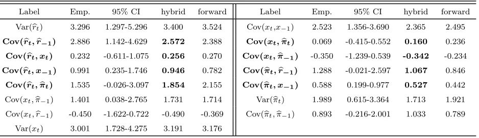
Table 3: Empirical and model-generated moments for inflation persistence: 15 moment conditions

Label Emp. 95% CI hybrid forward Label Emp. 95% CI hybrid forward

Var(rbt) 3.296 1.297-5.296 3.400 3.524 Cov(xt,x−1) 2.523 1.356-3.690 2.365 2.495

Cov(brt,rb₋₁) 2.886 1.142-4.629 2.572 2.388 Cov(xt,πbt) 0.069 -0.415-0.552 0.160 0.236

Cov(rbt, xt) 0.232 -0.611-1.075 0.256 0.270 Cov(xt,πb−1) -0.350 -1.239-0.539 -0.342 -0.234

Cov(rbt, x₋1) 0.991 0.235-1.746 0.946 0.782 Cov(πbt,rb₋1) 1.288 -0.021-2.597 1.067 0.846 Cov(rbt,πbt) 1.535 -0.026-3.097 1.854 2.155 Cov(πbt, x₋₁) 0.588 0.199-0.977 0.527 0.442 Cov(xt,bπ−1) 1.401 0.038-2.765 1.731 1.714 Var(bπ_t) 1.989 0.615-3.364 1.713 1.921

Cov(xt,br−1) -0.450 -1.622-0.722 -0.490 -0.369 Cov(bπt,bπ−1) 0.893 -0.216-2.001 1.033 0.789

Var(xt) 3.001 1.728-4.275 3.191 3.176

Note: 95% CI means the 95% asymptotic confidence intervals for empirical moments.

Next, we consider the same steps for the model comparison using the GM data. However, most parameter estimates of the two models do not differ too much. For example, the estimated value for the price indexation is close to zero in the hybrid variant of the model; i.e.αb = 0.105. Accordingly, the result of the formal test shows that the two models fit the data equally well. We find that the estimated QLR statistic is small: QLR = 0.17. The simulated 1% and 5% criteria for the hypothesis testing are 0.51 and 0.27, respectively; see the right panel of Figure 3 in appendix F. Therefore the null hypothesis cannot be rejected.

To save space, we do not report the model-generated moments for GM. Indeed, when we compare trajectories of the model-generated moments (i.e. hybrid and forward), the model covariance profiles almost overlap with each other. The two models provide a good fit to auto- and cross-covarainces at the short lag. In other words, we conclude that the two models are not significantly different at 5% level. We discuss the evaluation of the fit of the model using alternative moment conditions later, because the model has a bad fit to the sample autocovariances up to relatively large lags (two or three years).

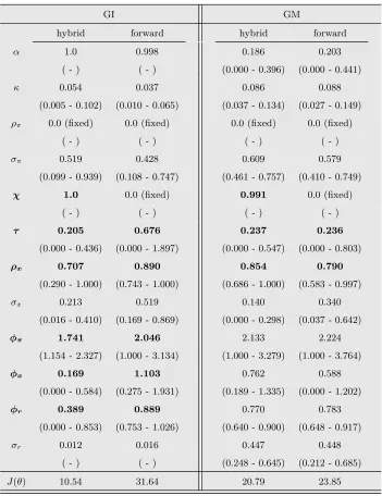
4.2.2 Assessing the fit of the model to output persistence: 15 moments

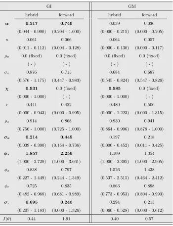
Turning to the output dynamics in the IS equation, we estimate the effects of habit persistence on the NKM. The estimated parameters for the model with or without a habit formation are presented in Table 4; in the purely forward-looking behaviorχis set to zero, whereas this parameter is subject to the estimation in the hybrid variant of the model. The MM estimates of the two models have almost similar values except for the degree of the supply shockσx, monetary policy shockσr and the Taylor rule coefficientφπ.

It can be seen from the GI data that the estimated demand shock is two times higher in an optimal con-sumption behavior without habit persistence than the other model (σbx= 0.45 (forward)>0.21 (hybrid)).

a simple rule of thumb behavior is not allowed in the IS equation. As a result, the persistence from the demand shocks also affects inflation dynamics while offsetting the effects of inherited persistence. This is indicated by a relatively moderate degree of backward-looking behavior; i.e.αb= 0.517 (hybrid) and 0.740 (forward). Moreover, concerning the hybrid model specification, which allows a fraction of consumers to have a rule of thumb behavior, the estimation results indicate a low value for the monetary coefficients on inflation; i.e.φbπ = 2.26 (forward)>1.86 (hybrid). Put differently, central banks react weakly to shocks

due to the fact that the transmission of the shocks endogenously affects the output persistence; since the parameter estimates are imprecise with a large confidence interval, however, we might raise doubts about appropriateness of this implication especially when the sample size is small. The reliability of the parameter estimates will be investigated later via a Monte Carlo study.

Table 4: Parameter estimates for output persistence with 15 moments

GI GM

hybrid forward hybrid forward

α 0.517 0.740 0.039 0.036

(0.044 - 0.990) (0.204 - 1.000) (0.000 - 0.215) (0.000 - 0.205)

κ 0.061 0.066 0.064 0.057

(0.011 - 0.112) (0.004 - 0.128) (0.000 - 0.130) (0.000 - 0.117)

ρπ 0.0 (fixed) 0.0 (fixed) 0.0 (fixed) 0.0 (fixed)

( - ) ( - ) ( - ) ( - )

σπ 0.876 0.715 0.684 0.687

(0.576 - 1.175) (0.447 - 0.983) (0.545 - 0.824) (0.547 - 0.826)

χ 0.931 0.0 (fixed) 0.585 0.0 (fixed)

(0.000 - 1.000) ( - ) (0.000 - 1.000) ( - )

τ 0.441 0.422 0.480 0.506

(0.000 - 0.943) (0.000 - 0.995) (0.000 - 1.223) (0.000 - 1.315)

ρx 0.914 0.868 0.930 0.941

(0.756 - 1.000) (0.725 - 1.000) (0.864 - 0.996) (0.878 - 1.000)

σx 0.214 0.445 0.197 0.218

(0.039 - 0.390) (0.154 - 0.736) (0.000 - 0.452) (0.011 - 0.425)

φπ 1.857 2.256 1.109 1.354

(1.000 - 2.729) (1.000 - 3.661) (1.000 - 2.395) (1.000 - 2.905)

φx 0.838 0.797 1.526 1.438

(0.227 - 1.449) (0.244 - 1.349) (0.537 - 2.515) (0.464 - 2.412)

φr 0.725 0.835 0.863 0.898

(0.482 - 0.968) (0.681 - 0.989) (0.773 - 0.953) (0.804 - 0.993)

σr 0.695 0.240 0.294 0.215

(0.207 - 1.183) (0.000 - 1.326) (0.060 - 0.528) (0.000 - 0.612)

J(θ) 0.44 1.91 0.40 0.57

Note: The discount factor parameterβis calibrated to 0.99. The 95% asymptotic confidence intervals are given

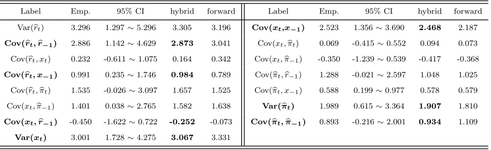
Now, we compute the loss function values to apply a formal test to the two specifications in the IS equation. In GI, these values are respectively 0.44 and 1.91 for the model with and without habit formation. The simulated 1% and 5% criteria for the hypothesis testing are 1.89 and 1.08, respectively; see the left panel of Figure 4 in appendix F. Since the estimated value for QLR exceeds the criterion at 5% level, we reject the null hypothesis that the two models are equivalent. This implies that the output dynamics are better approximated by the consumption behavior in a rule of thumb manner. This finding is shown in Table 5. For example, the hybrid variant of the model can almost provide perfect fit to the covariance profiles of (rt, xt−k), (xt, xt−k) and (πt, πt−k).

Table 5: Empirical and model-generated moments for output persistence: 15 moment conditions

Label Emp. 95% CI hybrid forward Label Emp. 95% CI hybrid forward

Var(rbt) 3.296 1.297∼5.296 3.305 3.196 Cov(xt,x−1) 2.523 1.356∼3.690 2.468 2.187

Cov(brt,rb₋₁) 2.886 1.142∼4.629 2.873 3.041 Cov(xt,πbt) 0.069 -0.415∼0.552 0.094 0.073

Cov(rbt, xt) 0.232 -0.611∼1.075 0.164 0.342 Cov(xt,πb−1) -0.350 -1.239_∼0.539 -0.417 -0.368

Cov(rbt, x₋₁) 0.991 0.235∼1.746 0.984 0.789 Cov(πbt,rb−1) 1.288 -0.021_∼2.597 1.048 1.025

Cov(rbt,bπt) 1.535 -0.026∼3.097 1.657 1.525 Cov(πbt, x−1) 0.588 0.199_∼0.977 0.578 0.579

Cov(xt,bπ−1) 1.401 0.038_∼2.765 1.582 1.638 Var(πbt) 1.989 0.615_∼3.364 1.907 1.810

Cov(xt,rb₋1) -0.450 -1.622∼0.722 -0.252 -0.073 Cov(πbt,πb₋1) 0.893 -0.216∼2.001 0.934 1.109

Var(xt) 3.001 1.728∼4.275 3.067 3.331

Note: 95% CI means the 95% asymptotic confidence intervals for empirical moments.

In the period of GM, the parameter estimates for the two models are found to be similar. This implies that the difference in the loss function values is small (i.e., QLR = 0.17). The simulated 1% and 5% criteria for the hypothesis testing are 7.58 and 12.37, respectively; see the right panel of Figure 4 in appendix F. We cannot reject the null hypothesis that the two models are equivalent. To save space, we do not report the model-generated moments for the GM period; the covariance profiles of the two models more or less overlap with each other.

4.3

Basic results on maximum likelihood estimation

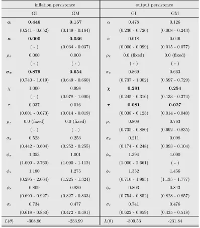
activity (i.e., the Phillips curve is flat). Hence, inflation dynamics in GI are primarily driven by intrinsic (moderate) and extrinsic (strong) persistence; i.e.αb= 0.446,bσπ = 0.879.

Table 6: ML estimates for inflation and output persistence

inflation persistence output persistence

GI GM GI GM

α 0.446 0.157 α 0.478 0.126

(0.241 - 0.652) (0.149 - 0.164) (0.230 - 0.726) (0.008 - 0.243)

κ 0.000 0.036 κ 0.018 0.046

( - ) (0.034 - 0.037) (0.000 - 0.099) (0.015 - 0.077)

ρπ 0.000 0.000 ρπ 0.0 (fixed) 0.0 (fixed)

( - ) ( - ) ( - ) ( - )

σπ 0.879 0.654 σπ 0.869 0.663

(0.740 - 1.019) (0.649 - 0.660) (0.737 - 1.002) (0.597 - 0.729)

χ 1.000 0.998 χ 0.281 0.254

( - ) (0.978 - 1.000) (0.245 - 0.316) (0.133 - 0.374)

τ 0.037 0.016 τ 0.081 0.027

(0.001 - 0.073) (0.014 - 0.019) (0.038 - 0.125) (0.014 - 0.040)

ρx 0.0 (fixed) 0.0 (fixed) ρx 0.808 0.763

( - ) ( - ) (0.735 - 0.880) (0.692 - 0.835)

σx 0.523 0.253 σx 0.211 0.098

(0.442 - 0.604) (0.252 - 0.255) (0.174 - 0.248) (0.093 - 0.104)

φπ 1.353 1.001 φπ 1.394 1.000

(1.000 - 2.760) (1.000 - 1.112) (1.000 - 2.661) ( - )

φx 1.180 1.275 φx 1.352 1.456

(0.295 - 2.064) (1.225 - 1.324) (0.710 - 1.995) (1.135 - 1.777)

φr 0.809 0.830 φr 0.803 0.843

(0.690 - 0.927) (0.827 - 0.833) (0.754 - 0.852) (0.828 - 0.857)

σr 0.734 0.477 σr 0.741 0.476

(0.618 - 0.850) (0.472 - 0.481) (0.622 - 0.859) (0.435 - 0.518)

L(θ) -308.86 -233.99 L(θ) -309.53 -231.84

Note: The discount factor parameterβis calibrated to 0.99. The 95% asymptotic confidence intervals are given

in brackets.

Overall, the slight difference between ML and MM can be attributed to the assumption of normality of the shocks; if the model is correctly specified, the ML estimation may be superior to the MM estimation. Since we do not know the true data generating process in almost all cases, however, MM is likely to be a relevant choice for evaluating the model’s goodness-of-fit to the data; the moment matching results in a closer fit to the sample autocovariance. The statistical efficiency and consistency of the parameter estimation adopted in this study will be investigated via a Monte Carlo study later.

Another important point is that the high dimension of the parameter space can induce multiple local minima in the likelihood function. If we change the starting values in optimization, we often obtain differ-ent values for the parameter estimation; more rigorous investigation with simulation-based optimization methods (i.e., simulated annealing, random search method) would be worthwhile. However, in the current study, we have a strong confidence in a global minimum for the parameter estimates, because we tested our empirical results with different starting values and found that they converge to a unique minimum. In this respect, the structural estimation based on the analytical solution of the system is able to overcome the parameter identification problems in a small-scale hybrid NKM. To make a more systemic investigation on our choice of moments, the next section examines the parameter estimation of the model using a large set of moment conditions.

4.4

Validity of extra moment conditions

In this section, we examine the sensitivity of the MM estimation to the chosen moment conditions. From this investigation, we will find that alternative moment conditions do not induce qualitative changes in the parameter estimation. To make our choice of moment conditions more reliable, we make a case for the vector autoregressive (VAR) model with lag 4 as a reference model; see appendix C for optimal lag selection criteria. Accordingly, we analyze the persistence of the macro data in the U.S. economy using auto- and cross-covariances up to lag 4.

4.4.1 Assessing the fit of the model to inflation persistence: 42 moments

With a focus on alternative moment conditions (42 moments), we now estimate two specifications of the NKM: forward-looking (α= 0) and hybrid case (i.e.αis a free parameter). In Table 7, we find evidence of strong backward-looking behavior in the NKPC;αb= 1.0. Moreover, the MM estimates with a small and large set of moments give qualitatively similar values except for the policy shock parameter (σr=0.0).8

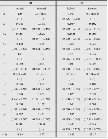
For example, in the model with purely forward-looking behavior, the effects of the inherited and extrinsic persistence play an important role in order to compensate for the absence of intrinsic persistence in the NKPC:κ= 0.155 (forward)>0.044 (hybrid), ρπ = 0.675 (forward)>0.0 (hybrid).

8

Indeed, ML would avoid such an estimate provided that there is a stochastic singularity with zero policy shock (i.e., the

Table 7: Parameter estimates for inflation persistence with 42 moments

GI GM

hybrid forward hybrid forward

α 1.0 _{0.0 (fixed) 0.509 0.0 (fixed)}

( - ) ( - ) (0.126 - 0.924) ( - )

κ 0.044 0.155 0.037 0.102

(0.018 - 0.069) (0.000 - 0.395) (0.000 - 0.075) (0.017 - 0.187)

ρπ 0.000 0.675 0.000 0.596

( - ) (0.387 - 0.964) (0.000 - 0.813) (0.367 - 0.825)

σπ 0.470 0.518 0.364 0.231

(0.000 - 1.686) (0.233 - 0.790) (0.048 - 0.680) (0.093 - 0.369)

χ 1.0 1.0 0.770 0.915

( - ) ( - ) (0.515 - 1.000) (0.518 - 1.000)

τ 0.092 0.063 0.020 0.027

(0.045 - 0.140) (0.008 - 0.118) (0.000 - 0.055) (0.000 - 0.074)

ρx 0.0 (fixed) 0.0 (fixed) 0.0 (fixed) 0.0 (fixed)

( - ) ( - ) ( - ) ( - )

σx 0.716 0.600 0.547 0.468

(0.462 - 0.970) (0.348 - 0.853) (0.202 - 0.820) (0.185 - 0.751)

φπ 1.740 1.809 2.025 2.218

(1.255 - 2.225) (1.221 - 2.397) (1.000 - 2.870) (1.141 - 3.114)

φx 0.080 0.157 0.563 0.564

(0.000 - 0.542) (0.000 - 0.528) (0.216 - 1.059) (0.154 - 0.974)

φr 0.267 0.458 0.765 0.732

(0.000 - 0.905) (0.224 - 0.692) (0.619 - 0.881) (0.592 - 0.872)

σr 0.000 0.000 0.486 0.545

( - ) ( - ) (0.303 - 0.727) (0.351 - 0.739)

J(θ) 11.93 42.77 23.97 27.47

Note: The discount factor parameterβis calibrated to 0.99. The 95% asymptotic confidence intervals are given

in brackets.

In the period of GI, the hybrid variant of NKP has a better goodness-of-fit to the data (J = 11.93) than the purely forward-looking version of the model (J = 42.77). As it is discussed above, the estimated AR (1) coefficient for the cost push shock has no influence on the hybrid NKPC;ρbπ = 0.0.9 The results also

show that inherited persistence has a smaller impact on the output dynamics in the hybrid variant of the model (bκ= 0.044). This implies that the persistence is best captured by the backward-looking behavior in the hybrid variant. As a result, we find almost perfect fit to the comovements between inflation and output from the hybrid NKM.

1 4 8 12 −2 0 2 4 6 Cov(r

t, rt−k)

1 4 8 12 −2

0 2 4

Cov(r

t, xt−k)

1 4 8 12 −2

0 2

Cov(r

t, πt−k)

1 4 8 12 −4

−2 0 2

Cov(x

t, rt−k)

1 4 8 12 −5

0 5

Cov(x

t, xt−k)

1 4 8 12 −4

−2 0 2

Cov(x

t, πt−k)

1 4 8 12 −2

0 2

Cov(π

t, rt−k)

1 4 8 12 −2

0 2 4

Cov(π

t, xt−k)

1 4 8 12 −1 0 1 2 3 Cov(π

t, πt−k)

VAR(4) +z

95% CI

−z

95% CI

forward (α=0) hybrid (α=1)

Figure 1: Covariance profiles for inflation persistence in GI (dashed: empirical,△: hybrid, *: forward)

Note: The empirical auto- and cross-covariances are computed using an unrestricted fourth-order vector

au-toregression (VAR) model. The asymptotic 95% confidence bands are constructed following Coenen (2005).

In order to examine the significant difference of the fit of the two models, we subtract the objective function value of purely forward-looking NKM from the one of its hybrid variant; i.e. QLR = 30.83. According to the simulated test distribution, critical values for the 99% and 95% confidence intervals

9

The estimated value for the parameterσr hit the boundary. This makes the objective function ill-behaved and partial

derivatives numerically unstable. We set it to zero and compute the numerical derivatives of the other parameters for the

are 16.99 and 9.96, respectively (see the left panel of Figure 5 in appendix F). Since the test statistic exceeds the critical value at 5% level, we proceed to take the second step of the hypothesis testing, which asymptotically evaluates the estimated moments of two models from the profiles of empirical data.

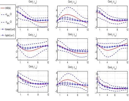
1 4 8 12

−2 0 2

Cov(r

t, rt−k)

1 4 8 12

−1 0 1

Cov(r

t, xt−k)

1 4 8 12

−0.5 0 0.5

Cov(r

t, πt−k)

1 4 8 12

−1 0 1

Cov(x

t, rt−k)

1 4 8 12

−1 0 1 2

Cov(x

t, xt−k)

1 4 8 12

−0.5 0 0.5

Cov(x

t, πt−k)

1 4 8 12

−0.5 0 0.5

Cov(π

t, rt−k)

1 4 8 12

−0.5 0 0.5

Cov(π

t, xt−k)

1 4 8 12

−0.5 0 0.5 1

Cov(π

t, πt−k)

VAR(4)

+z

95% CI

−z

95% CI

forward (α=0)

hybrid (α=0.51)

Figure 2: Covariance profiles for inflation persistence in GM (dashed: empirical,△: hybrid, *: forward)

Note: The empirical auto- and cross-covariances are computed using an unrestricted fourth-order vector

au-toregression (VAR) model. The asymptotic 95% confidence bands are constructed following Coenen (2005).

In the second step of the formal test, we examine the uncertainty of the estimated difference between the two models for evaluating their fit to the data. We compute the plug-in estimate ofwb0(2.54). Under the

null hypothesis, the test static follows a standard normal distribution; i.e.√T·QLR(θA_{, θ}B_{)∼N(0, w}2 0).

The estimate of√T ·QLR/wb is 1.37, which is smaller than a critical value at the 5% significance level of the two-tailed test. Therefore the results show that both models have the same goodness-of-fit to the profile of the empirical moments, and the null hypothesis cannot be rejected.10 _{Figure 1 depicts the}

model-generated moment conditions at three years for GI and contrasts them with the empirical counterparts of the VAR (4) model. Indeed, a visual inspection of this figure indicates that the two models have different

10

This statistical inference does not remain the same if the price indexation parameter is allowed to exceed unity. The

moments, but their matching to the empirical counterparts is not significantly different.

In the period of GM (Table 7), it is shown that the hybrid variant of NKP fits the data better (23.97). The estimation results provide evidence of the (strong) inherited and extrinsic persistence in the model with purely forward-looking behavior, because these can offset the impact of inherited persistence on the output dynamics; i.e.bκ= 0.102 (forward) >0.037 (hybrid), ρbπ = 0.596 (forward)> 0.0 (hybrid).

However, the other parameter estimates are not different in both specifications.

These empirical findings also seem to strengthen the relevance of backward-looking behavior for the GM data. However, the difference between the two models (3.49) does not exceed the critical value for the 95% confidence intervals in the formal test; i.e., critical values for 99% and 95% confidence intervals are 38.39 and 21.46, respectively; also see the right panel of Figure 5 in appendix F. Put differently, the effects of inherited persistence on inflation can be adequately replaced by the inherited and extrinsic persistence, which cannot distinguish between the sources of the persistence in the NKPC. Therefore we do not proceed to take the second step of the model comparison method and conclude that the null hypothesis cannot be rejected. Figure 2 depicts the model-generated moment conditions at three years for the GM data; the comparison between the model-generated and empirical moments by a VAR (4) process is displayed here.

4.4.2 Assessing the fit of the model to output persistence: 42 moments

Table 8 reports the MM estimation for the output persistence using alternative moment conditions. The results show that the output dynamics are strongly influenced by the inherited persistence. Indeed, the intertemporal elasticity of substitution of the two models has high estimated values with the data: e.g. in GI, bτ = 0.205 (hybrid), 0.676 (forward). In addition, we find that all the estimated values for ρx

exceed 0.7. Especially regarding the GI data, this value increases substantially in the model with purely forward-looking expectations, which can cover the absence of intrinsic persistence in the IS equation; i.e.

χ=0.0 (fixed), bτ = 0.676.

Another point worthwhile mentioning here is that the estimation results of the purely forward-looking model indicate high monetary policy coefficients on interest rate, inflation and output in GI; i.e.φbπ = 2.05,

b

φx= 1.10,φbr= 0.89. Moreover, in the hybrid variant, the parameterχis almost a corner solution for both

the GI and GM data, which strengthens a rule of thumb behavior in consumption. This implies that the rule of thumb behavior reinforces the degree of endogenous persistence in the output dynamics. However, as long as the model predicts that the optimal behavior of household is described by consumption without a simple rule of thumb behavior (χ = 0), the result indicates the strong degree of the demand shocks; the estimated value is more than twice as high as the one of the hybrid model; i.e.bσx=0.519 (forward)>

0.213 (hybrid) for GI, 0.340 (forward)>0.140 (hybrid) for GM.

two models have different moments. In the second step, we estimate√T·QLR/wbwhich is 1.02. However, this value does not exceed the criterion in the standard normal distribution. As a result, we conclude that there is no significant difference between two models in matching the empirical moments; i.e. the two models have different moments, but an equivalent fit to the empirical moments. To save space, we do not provide the model covariance profiles for the output persistence. Note here that the result of the MM estimation with a large set of moments provides a closer fit to the sample auto- and cross-covariances up to large lags.

Table 8: Parameter estimates for output persistence with 42 moments

GI GM

hybrid forward hybrid forward

α 1.0 0.998 0.186 0.203

( - ) ( - ) (0.000 - 0.396) (0.000 - 0.441)

κ 0.054 0.037 0.086 0.088

(0.005 - 0.102) (0.010 - 0.065) (0.037 - 0.134) (0.027 - 0.149)

ρπ 0.0 (fixed) 0.0 (fixed) 0.0 (fixed) 0.0 (fixed)

( - ) ( - ) ( - ) ( - )

σπ 0.519 0.428 0.609 0.579

(0.099 - 0.939) (0.108 - 0.747) (0.461 - 0.757) (0.410 - 0.749)

χ 1.0 0.0 (fixed) 0.991 0.0 (fixed)

( - ) ( - ) ( - ) ( - )

τ 0.205 0.676 0.237 0.236

(0.000 - 0.436) (0.000 - 1.897) (0.000 - 0.547) (0.000 - 0.803)

ρx 0.707 0.890 0.854 0.790

(0.290 - 1.000) (0.743 - 1.000) (0.686 - 1.000) (0.583 - 0.997)

σx 0.213 0.519 0.140 0.340

(0.016 - 0.410) (0.169 - 0.869) (0.000 - 0.298) (0.037 - 0.642)

φπ 1.741 2.046 2.133 2.224

(1.154 - 2.327) (1.000 - 3.134) (1.000 - 3.279) (1.000 - 3.764)

φx 0.169 1.103 0.762 0.588

(0.000 - 0.584) (0.275 - 1.931) (0.189 - 1.335) (0.000 - 1.202)

φr 0.389 0.889 0.770 0.783

(0.000 - 0.853) (0.753 - 1.026) (0.640 - 0.900) (0.648 - 0.917)

σr 0.012 0.016 0.447 0.448

( - ) ( - ) (0.248 - 0.645) (0.212 - 0.685)

J(θ) 10.54 31.64 20.79 23.85

Note: The discount factor parameterβis calibrated to 0.99. The 95% asymptotic confidence intervals are given

in brackets.

interior point. The model without habit persistence is nested within the other. Next, we compute the difference between the objective function values of the two models (QLR = 3.06). Then this value is used to evaluate the null hypothesis of the equal fit of the two models. Since the 5% and 1% criteria for the hypothesis testing are 18.52 and 29.05, respectively (see the right panel of Figure 7), the null hypothesis cannot be rejected. Therefore we conclude that two models have an equal fit to the empirical moments.

5

Attaining efficiency from moment conditions

In this section, first, we study the finite sample properties of MM and ML; in addition, we investigate the effect of model misspecification on the parameter estimation. Second, we discuss the empirical performance of the formal test of HMT along the lines of the Akaike’s and the Bayesian information criterion.

5.1

Monte Carlo study

The Monte Carlo (MC) experiment attempts to clearly demonstrate the statistical efficiency of the estima-tion methods, which are used in the previous secestima-tion. In this way, we aim to investigate the role of choice of moments and its influence on the parameter estimation. To begin, we consider the model specification of inflation persistence as the true date generating process; we simulate the artificial economy by using the parameters near to the results of the MM estimation with 15 moments (see Table 2): e.g. high de-gree of backward-looking behavior (α=0.750), moderate inherited persistence (κ=0.050) and no extrinsic persistence (ρπ=0.0). Next, we generate 1,000 data sets each consisting of 550 observations. The first

50 observations are removed as a transient period. Three sample sizes are considered: 100, 200 and 500. We use the Matlab R2010a for this MC study. In optimization, we use the unconstrained minimization

"fminicon"with the algorithm ’interior-point’; maximum iteration and tolerance level are set to 500 and 10−6_{, respectively.}

We conduct the MC experiments by considering two cases of model specification; i.e. correctly specified and misspecified. In the former, we discuss the finite sample properties of the MM and ML estimation. Turning to the latter, we consider the model with purely forward-looking expectations and examine the degree of bias in the parameter estimates; i.e. (1) to what extent the extrinsic persistence (ρπ) is inflated

due to the misspecification and (2) to what extent the model misspecification affects the estimates for the other structural parameters.

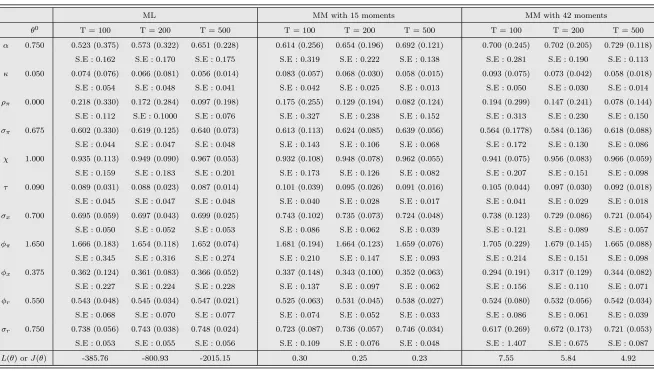
The main findings for the correctly specified case in Table 9 can be summarized as follows:

• For both ML and MM, the estimate of the price indexation parameterαis downward-biased, whereas the AR (1) coefficient of inflation shocksρπ is estimated to be positive.

• ML has slightly poorer finite sample properties than MM. This implies that conventional Gaussian asymptotic approximation to the sample distribution is not as much precise as MM, as long as the sample size is small.

• The asymptotic efficiency of the ML estimation appears superior to MM, since the mean of standard errors over 1000 estimations shows that the confidence intervals for the MM estimates are noticeably narrow. However, the large sample size remarkably improves the asymptotic efficiency of MM with 15 and 42 moments; e.g. T=500.

of statistical inference for the behavior of economic agents (i.e. backward- or forward-looking) comes at the cost of allowing for large uncertainty in the estimates of other structural parameters; in other words, incorporating more second moments in the objective function improves the fit of the model to the persistence of inflation dynamics, but reduces efficiency in the other structural parameters.

• The results using MM with 42 moments show that we obtain the large asymptotic error for the policy shock parameter σr; i.e. S.E = 1.407 for T=100. This is attributed to the fact that the

estimated values sometimes hit the boundary (i.e.σr= 0.0), which makes the numerical derivative

of the moments unstable. This problem does not occur in the case where the large sample size is used (e.g. T=500).

Turning to the misspecified case, the MC results show that there is a high correlation between the price indexation and AR (1) coefficient of the supply shocks; see appendix G. Indeed, it is shown in Table G.2 that the AR (1) coefficient is strongly upward-biased for both MM and ML. The parameter estimates offset the effects of intrinsic persistence on the inflation dynamics; e.g.ρπ= 0.616 (ML), 0.632 (MM with

15 moments), 0.598 (MM with 42 moments) when the sample size is 100. The large sample size does not correct the bias of this parameter. Fortunately, the other structural parameters are not influenced by the model misspecification; i.e. we obtain the parameter estimation near to the true ones by using both MM and ML. They converge at some reasonable rate towards the true parameters as the sample size gets larger (consistency).

Similarly, the degree of the inflation shockσπ is more or less downward-biased. In addition, the slope

Table 9: The Monte Carlo results on the MM and ML estimates, ( ): root mean square error, S.E : mean of standard error

ML MM with 15 moments MM with 42 moments

θ0

T = 100 T = 200 T = 500 T = 100 T = 200 T = 500 T = 100 T = 200 T = 500

α 0.750 0.523 (0.375) 0.573 (0.322) 0.651 (0.228) 0.614 (0.256) 0.654 (0.196) 0.692 (0.121) 0.700 (0.245) 0.702 (0.205) 0.729 (0.118)

S.E : 0.162 S.E : 0.170 S.E : 0.175 S.E : 0.319 S.E : 0.222 S.E : 0.138 S.E : 0.281 S.E : 0.190 S.E : 0.113

κ 0.050 0.074 (0.076) 0.066 (0.081) 0.056 (0.014) 0.083 (0.057) 0.068 (0.030) 0.058 (0.015) 0.093 (0.075) 0.073 (0.042) 0.058 (0.018)

S.E : 0.054 S.E : 0.048 S.E : 0.041 S.E : 0.042 S.E : 0.025 S.E : 0.013 S.E : 0.050 S.E : 0.030 S.E : 0.014

ρπ 0.000 0.218 (0.330) 0.172 (0.284) 0.097 (0.198) 0.175 (0.255) 0.129 (0.194) 0.082 (0.124) 0.194 (0.299) 0.147 (0.241) 0.078 (0.144)

S.E : 0.112 S.E : 0.1000 S.E : 0.076 S.E : 0.327 S.E : 0.238 S.E : 0.152 S.E : 0.313 S.E : 0.230 S.E : 0.150

σπ 0.675 0.602 (0.330) 0.619 (0.125) 0.640 (0.073) 0.613 (0.113) 0.624 (0.085) 0.639 (0.056) 0.564 (0.1778) 0.584 (0.136) 0.618 (0.088)

S.E : 0.044 S.E : 0.047 S.E : 0.048 S.E : 0.143 S.E : 0.106 S.E : 0.068 S.E : 0.172 S.E : 0.130 S.E : 0.086

χ 1.000 0.935 (0.113) 0.949 (0.090) 0.967 (0.053) 0.932 (0.108) 0.948 (0.078) 0.962 (0.055) 0.941 (0.075) 0.956 (0.083) 0.966 (0.059)

S.E : 0.159 S.E : 0.183 S.E : 0.201 S.E : 0.173 S.E : 0.126 S.E : 0.082 S.E : 0.207 S.E : 0.151 S.E : 0.098

τ 0.090 0.089 (0.031) 0.088 (0.023) 0.087 (0.014) 0.101 (0.039) 0.095 (0.026) 0.091 (0.016) 0.105 (0.044) 0.097 (0.030) 0.092 (0.018)

S.E : 0.045 S.E : 0.047 S.E : 0.048 S.E : 0.040 S.E : 0.028 S.E : 0.017 S.E : 0.041 S.E : 0.029 S.E : 0.018

σx 0.700 0.695 (0.059) 0.697 (0.043) 0.699 (0.025) 0.743 (0.102) 0.735 (0.073) 0.724 (0.048) 0.738 (0.123) 0.729 (0.086) 0.721 (0.054)

S.E : 0.050 S.E : 0.052 S.E : 0.053 S.E : 0.086 S.E : 0.062 S.E : 0.039 S.E : 0.121 S.E : 0.089 S.E : 0.057

φπ 1.650 1.666 (0.183) 1.654 (0.118) 1.652 (0.074) 1.681 (0.194) 1.664 (0.123) 1.659 (0.076) 1.705 (0.229) 1.679 (0.145) 1.665 (0.088)

S.E : 0.345 S.E : 0.316 S.E : 0.274 S.E : 0.210 S.E : 0.147 S.E : 0.093 S.E : 0.214 S.E : 0.151 S.E : 0.098

φx 0.375 0.362 (0.124) 0.361 (0.083) 0.366 (0.052) 0.337 (0.148) 0.343 (0.100) 0.352 (0.063) 0.294 (0.191) 0.317 (0.129) 0.344 (0.082)

S.E : 0.227 S.E : 0.224 S.E : 0.228 S.E : 0.137 S.E : 0.097 S.E : 0.062 S.E : 0.156 S.E : 0.110 S.E : 0.071

φr 0.550 0.543 (0.048) 0.545 (0.034) 0.547 (0.021) 0.525 (0.063) 0.531 (0.045) 0.538 (0.027) 0.524 (0.080) 0.532 (0.056) 0.542 (0.034)

S.E : 0.068 S.E : 0.070 S.E : 0.077 S.E : 0.074 S.E : 0.052 S.E : 0.033 S.E : 0.086 S.E : 0.061 S.E : 0.039

σr 0.750 0.738 (0.056) 0.743 (0.038) 0.748 (0.024) 0.723 (0.087) 0.736 (0.057) 0.746 (0.034) 0.617 (0.269) 0.672 (0.173) 0.721 (0.053)

S.E : 0.053 S.E : 0.055 S.E : 0.056 S.E : 0.109 S.E : 0.076 S.E : 0.048 S.E : 1.407 S.E : 0.675 S.E : 0.087

L(θ) orJ(θ) -385.76 -800.93 -2015.15 0.30 0.25 0.23 7.55 5.84 4.92

2

5.2

Model selection and discussion

From the empirical investigation using MM with a large set of moments, we found that the statistical power of the model comparison test is weak and the result becomes inconclusive; in this case, we treat two models as being overlapping. Note here that we use the small sample to estimate the parameters of the NKM in which the asymptotic test of the model comparison is likely to make a Type II error; i.e. we accept the null hypothesis when the equal fit of moments is false.11

Table 10: Model selection using information criteria: inflation persistence GI (T=78) GM (T=99) ML hybrid forward ML hybrid forward

L(θ)/T -3.96 -4.41 -4.82 -2.36 -2.69 -2.69 AIC 8.20 9.02 9.90 4.95 5.61 5.58 BIC 8.53 9.43 10.20 5.24 5.90 5.84 Ranking 1 2 3 1 3 2

Note: The backward- and forward-looking behaviors are examined using the MM estimation with auto- and cross-covariances at lag 1.

To make the formal test more elaborate, we rank the model according to the well-known information criteria in the ML estimation. For this purpose, we suppose that the parameter estimates using MM are to be a possible minimum point in the likelihood function. Table 10 and 11 report the mean value for the log-likelihood and the model selection criterion: the cases of inflation and output persistence, respectively. Here we present MM with a small set of the moment conditions (auto- and cross-covariances at lag 1), because MM with alternative moments (auto- and cross-covariances at lag 4) yields the zero policy shock for the GI data.

According to AIC and BIC, by definition, we prefer the ML over the MM estimation with 15 moments for both GI and GM data. If the assumption of normality is not violated and the model is correctly specified, we can conclude that the ML estimation is the most efficient; this statistical inference is verified by the MC study in the previous section. Nevertheless, the AIC and BIC of the MM estimation do not differ too much from the ML estimation. This implies that matching the auto- and cross-covariances at lag 1 can provide more or less the same efficiency as the ML approach. Also the statistical inference for the behavior of economic agents does not change; i.e. the hybrid variant can approximate the dynamics in inflation and output better than the model with purely forward-looking behavior when fitting the GI data: e.g. AIC = 9.02 (hybrid)<9.90 (forward). On the other hand, the inconclusive result using the GM data shows that the price-setting rule without indexation to past inflation (or purely forward-looking) is preferred due to its parsimonious description of the data: i.e. BIC = 5.90 (hybrid)>5.84 (forward).

11

Marmer and Otsu (2012) discuss the general optimality of comparison of misspecified models and propose a feasible

Table 11: Model selection using information criteria: output persistence GI (T=78) GM (T=99) ML hybrid forward ML hybrid forward

L(θ)/T -3.97 -4.62 -7.88 -2.34 -3.09 -4.22 AIC 8.22 9.51 16.01 4.91 6.41 8.64 BIC 8.55 9.85 16.31 5.19 6.69 8.90 Ranking 1 2 3 1 2 3

Note: The backward- and forward-looking behaviors are examined using the MM estimation with auto- and cross-covariances at lag 1.

In Table 11, we have found essentially similar results for the output persistence; the results of the model comparison indicate that the backward-looking behavior in the IS equation is more appropriate for both GI and GM data. These exercises indicate that ML and MM have basically equivalent properties in statistical inference; they result in the same conclusion for the model comparison.12 _{In other words, as}

long as the chosen moment conditions are efficient, we do not find any difference between the formal tests from the ML and MM estimations. Nonetheless, the formal test of HMT will be a very convenient tool if we are interested in a certain dimension of the data generating process and attempt to find significant differences between two models along the lines of chosen moment conditions.

In addition, we can see from our empirical application that the moment-matching method achieves a high accuracy in taking the models to the data, but the parameter estimation becomes more uncertain than ML; i.e. wide confidence intervals. Indeed, this empirical observations can relate to the uncertainty of the model selection for the lagged term in the NKPC and the IS equation. Moreover, in our empirical application, if we include additional second moments in the objective function, this improves the perfor-mance of the model to fit inflation and output persistence, but will make the comparison results of two models inconclusive. The take-home message from this analysis is that we should take into account the power of the test for certain choices of moment conditions.

To address this issue on the trade-off between the fit of the model and the power of the formal test, we would evaluate the empirical performance of competing models in terms of their predictive power. Alternatively, we can adopt some parts of model specifications and indicate to what extent the model selection procedure can be influenced by the model combination. For example, the method of the model averaging is proven to be a useful tool in a Bayesian approach. The inclusion of this concept into the model comparison will challenge the current framework for misspecified models.

12

However, remember that according to the formal test of HMT, the better fit of the hybrid variant is not significantly

superior to the other model when the GM data is used. In this sense, the model comparison of HMT is more concerned with

the accuracy of the approximation to the underlying data generating process rather than a direct comparison between the

6

Conclusion

This paper considered the structural estimation of the NKM where we conducted a formal comparison of the model with purely forward-looking behavior and its hybrid variant. Especially, we examined the importance of the future expected and lagged values in the inflation and output dynamics using US data; i.e. forward- and backward-looking behavior in the NKPC and the IS equation. The models are estimated by the classical estimation methods of MM and ML. In the former, we derived the analytical moments of the auto- and cross-covariances from a linear system of the NKM; we estimated the the parameters by matching the model-generated moments with their empirical counterparts. These empirical findings are compared with the ML estimation while their sensitivity to the moment conditions is also examined.

According to the estimated loss function values obtained by MM, we evaluated two competing models using the formal test of HMT when they are overlapping or one model is nested within another. The empirical results show that the inclusion of a lagged term in the NKPC and the IS equation improves the model’s empirical performance. In other words, the backward-looking behavior in the NKM plays an important role in approximating the persistence of inflation and output. This result suggests intrinsic persistence as the main source of the inflation and output dynamics in GI. However, in GM, we cannot reject the null hypothesis at 5% level, because the model with purely forward-looking expectations and its hybrid variant have an equal fit to the data. These empirical findings are verified using the MC experiments; we investigated the statistical efficiency of the estimators and the implications for the model selection.

References

Altonji, J. and Segal, L. (1996): Small-sample bias in GMM estimation of covariance structures.

Journal of Business and Economic Statistics, 14, 353–366.

Amato, J.D. and Laubach, T. (2003): Rule-of-thumb behaviour and monetary policy. European

Economic Review, Vol. 47(5), pp. 791–831.

Amato, J.D. and Laubach, T. (2004): Implications of habit formation for optimal monetary policy.

Journal of Monetary Economics, Vol. 51, pp. 305–325.

Anatolyev, S. and Gospodinov, N. (2011): Methods for Estimation and Inference in Modern

Econometrics. New York: A Chapman and Hall Book.

Andrews, D. (1991), Heteroskedasticity and autocorrelation consistent covariance matrix estimation.

Econometrica, Vol. 59, pp. 817–858.

Binder, M. and Pesaran, H.(1995): Multivariate Rational Expectations Models and Macroeconomic

Modeling: a Review and Some Insights, In: Pesaran, M.H. and Wickens, M. (ed.), Handbook of Applied

Econometrics. Oxford: Basil Blackwell, pp. 139–187.

Caldara, D., Fernandez-Villaverde, J., Rubio-Ramirez, J. and Yao, W. (2012): Computing

DSGE models with recursive preferences and stochastic volatility. Review of Economic Dynamics, Vol. 15(2), pp. 188–206.

Canova, F. and Sala, L.(2009): Back to square one: identification issues in DSGE models. Journal

of Monetary Economics, Vol. 56(4), pp. 431–449.

Carrillo, J.A., F´eve, P. and Matheron J. (2007): Monetary policy inertia or persistent shocks: a

DSGE analysis. International Journal of Central Banking, Vol. 3(2), pp. 1–38.

Castelnuovo, E. (2010): Trend inflation and macroeconomic volatilities in the Post WWII U.S.

economy. North American Journal of Economics and Finance, Vol. 21, pp. 19–33.

Christiano, L., Eichenbaum, M. and C. Evans(2005): Nominal rigidities and the dynamic effects

of a shock to monetary policy. Journal of Political Economy Vol. 113(1), pp. 1–45.

Clarida, R., Gali, J. and Gertler, M.(2000): Monetary policy rules and macroeconomic stability: