Numerical Experiments Using MATLAB: Superconvergence of Nonconforming Finite Element Approximation for Second Order Elliptic Problems

(1)

http://www.scirp.org/journal/am ISSN Online: 2152-7393 ISSN Print: 2152-7385

Numerical Experiments Using MATLAB:

Superconvergence of Nonconforming Finite

Element Approximation for Second-Order Elliptic

Problems

Anna Harris1*, Stephen Harris2, Danielle Rauls1

1_{Department of Mathematics and Computer Science, University of Arkansas at Pine Bluff, Pine Bluff, Arkansas, USA} 2_{US Food and Drug Administration, National Center for Toxicology Research, Jefferson, Arkansas, USA}

Abstract

The superconvergence in the finite element method is a phenomenon in which the finite element approximation converges to the exact solution at a rate higher than the optimal order error estimate. Wang proposed and analyzed superconvergence of the conforming finite element method by L2_{-projections. However, since the conforming} finite element method (CFEM) requires a strong continuity, it is not easy to con-struct such finite elements for the complex partial differential equations. Thus, the nonconforming finite element method (NCFEM) is more appealing computationally due to better stability and flexibility properties compared to CFEM. The objective of this paper is to establish a general superconvergence result for the nonconforming finite element approximations for second-order elliptic problems by L2_-projection methods by applying the idea presented in Wang. MATLAB codes are published at https://github.com/annaleeharris/Superconvergence-NCFEM for anyone to use and to study. The results of numerical experiments show great promise for the robust-ness, reliability, flexibility and accuracy of superconvergence in NCFEM by L2_- projections.

Keywords

Nonconforming Finite Element Methods, Superconvergence, L2_-Projection, Second-Order Elliptic Equation

1. Introduction

The conforming finite element method (CFEM) requires a strong continuity; hence it is not easy to construct such finite elements for the complex partial differential equations.

How to cite this paper: Harris, A., Harris, S. and Rauls, D. (2016) Numerical Experi-ments Using MATLAB: Superconvergence of Nonconforming Finite Element Approxi-mation for Second-Order Elliptic Problems.

Applied Mathematics, 7, 2174-2182.

http://dx.doi.org/10.4236/am.2016.717173

Received: September 20, 2016 Accepted: November 19, 2016 Published: November 22, 2016

(2)

The nonconforming finite element method (NCFEM) is more appealing computation-ally due to better stability and flexibility properties compared to CFEM [1][2][3]. The superconvergence in the finite element method is a phenomenon in which the finite element approximation converges to the exact solution at a rate higher than the optimal order error estimate. Wang proposed and analyzed superconvergence of the conform-ing finite element method by L2_{-projections. The main idea behind the L}2_{-projections is} to project the finite element solution to another finite element space with a coarse mesh and a higher order of polynomials.

The objective of this paper is to establish a general superconvergence result for the nonconforming finite element approximations for second-order elliptic problems by L2_{-projection methods by applying the idea presented in Wang}_[4]_.

This paper is organized as follows. In Section 2, we present a review for the nonconforming finite element method for the second-order elliptic problem. In Section 3, we develop a general theory of superconvergence by following the idea presented in Wang [4]. In Section 4, we perform numerical experiments to support the theoretical results. Numerical experiements of superconvergence of NCFEM are performed in MATLAB and its codes are posted at

https://github.com/annaleeharris/Superconvergence-NCFEM for anyone to use and to study.

2. NCFEM for the Second-Order Elliptic Problem

Consider the second-order elliptic problem with the Dirichlet boundary condition which seeks 1

( )

u∈H Ω satisfying

in ,

0 on ,

u f

u

∆ = Ω

= ∂Ω (1) where ∆_{is the Laplacian operator,}Ω_{is a bounded, connected, and open subset of}

2

R , ∂Ω is a Lipschitz continuous boundary, and a given function f is the external force.

A variational formulation of (1) seeks 1

( )

0

u∈H Ω such that

( ) (

)

1

( )

0

, , , ,

a u v = f v ∀ ∈v H Ω

where

( ) (

, ,

)

d .

a u v u v u v

Ω

= ∇ ∇ = ∇ ⋅ ∇ Ω

_∫

Let h be a quasi-uniform, i.e., it is regular and satisfies the inverse assumption [5], triangulation of Ω_with diam K

( )

≤h K, ∈h. Let P Kk

( )

be the space of polynomials of degree at most k with k≥0 on K. Let

ε

_h denote the union of the boun-

daries of all elements K∈h and let 0

\

h h

ε =ε ∂Ω_{be the collection of all interior} edges. Assume that the polynomial space in the construction of Vh contains P Kk

( )

,

1

k≥ . Define the finite element space Vh associated with h as

( )

{

}

2

0

: | , , is continuous at the middle point of

, and is zero at the middle point of boundary edge on .

h K k h

h

V v L v P K K v

e ε v e

= ∈ Ω ∈ ∀ ∈

∈ ∂Ω

(3)

The finite element space Vh is assumed to satisfy the following approximation property for any m 1

( )

u∈H + Ω [6]:

(

)

1

1 1

inf , 0 .

h

m m

v V u v h u v Ch u m k

+ +

∈ − + − ≤ ≤ ≤ (2)

The nonconforming finite element approximation problem (2) seeks uh∈Vh such that

(

,

) (

,

)

, ,

h h h

a u v = f v ∀ ∈v V (3)

where

(

,

)

(

,

)

d .

h h

h h h K K h

K K

a u v u v u v x

∈ ∈

=

∑

∇ ∇ =

∑ ∫

∇ ⋅∇

 

A well known error estimate for the finite element approximation solution

u

h is the following [7]:

1 1

1, ,

k

h h h k

u−u +h u−u ≤Ch+ u ₊ (4)

where C is a constant independent of the mesh size h.

To apply the superconvergence of finite element approximation, we assume that domain Ω_{is so regular that it ensures a} Hs,s≥1, regularity for the solution of (2).

In other words, for any s 2

( )

f ∈H − Ω the problem (2) has a unique solution

( )

1 0

u∈H Ω satisfying the following a priori estimate

( )

2

2, , 1,

s

s s

u ≤C f ₋ ∀ ∈f H − Ω s≥ (5)

where C is a constant independent of data f.

3. Superconvergence of NCFEM

Let τ be another finite element partition with coarse mesh size τ where hτ.

Assume that τ _{and h have the following relation:}

( )

, 0,1 .

hα

τ= α∈ ₍₆₎ Let V_τ be any finite element space consisting of piecewise polynomial of degree r

associated with the partition τ. Define Qτ to be the L2-projection from L2

( )

Ω

onto the finite element space V_τ. The finite element space Vτ is defined as follows:

( )

{

2

}

: |K r , .

Vτ = v∈L Ω v ∈P K ∀ ∈K τ

The following lemma will provide an error estimate for Q uτ −Q uτ h.

Lemma 1 Assume that the second-order elliptic problem (2) holds (5) with 1≤ ≤ +s k 1 and Vτ ⊂Hs−2

( )

Ω . Then there exists a constant C independent of h and

τ_{such that}

( ) 1 min 0,2

1,

k s s

h k

Q u_τ −Q u_τ ≤Ch+ − +α − u ₊ (7)

(4)

Proof. Using the definition of ⋅ and Q_τ, we have

( )

(

)

2 _, ₁

sup ,

h h

L

Q u_τ Q u_τ Q u_τ Q u_τ

φ φ

φ

∈ Ω =

− = −

and

(

Q uτ −Q uτ h,φ

) (

= u−u Qh, τφ

)

.

Then

( )

(

)

2 _, ₁

sup , .

h h

L

Q u_τ Q u_τ u u Q_τ

φ φ

φ

∈ Ω =

− = − ₍₈₎

Consider the following problem:

in ,

0 on .

w Q

w

τφ

−∆ = Ω

= ∂Ω (9) Multiplying the second-order elliptic Equation (1) by v and integrating it over Ω give

( )

, ,

(

,

)

,

h

h K

K

a u v u v _∂ f v

∈

−

∑

∇ ⋅n =

 (10) where n is the unit outward normal.

Subtract (3) from the above Equation (10) gives

(

,

)

, , .

h

h h K h

K

a u u v u v_∂ v V

∈

− =

∑

∇ ⋅n ∀ ∈

 (11)

Multiplying (9) by u−uh, integrating it over Ω, adding and subtracting wI∈Vh, and using the result (11) we have

(

) (

)

(

)

(

)

(

)

(

)

(

)

, , , , , , , , , , , , . h h h h h h h

h h h K

K

h I I h h K

K

h I h h I h h K

K

h I h I K h K

K K

Q u u w u u

a w u u w u u

a w w w u u w u u

a w w u u a w u u w u u

a w w u u u w w u u

τφ ∂ ∈ ∂ ∈ ∂ ∈ ∂ ∂ ∈ ∈ − = −∆ − = − − ∇ ⋅ − = − + − − ∇ ⋅ − = − − + − − ∇ ⋅ − = − − + ∇ ⋅ − ∇ ⋅ −

∑

n n n n n     

The line integrals of the above equations are approximated in [6] as follows: 1

1

, ,

h

k s

I K k s

K

u w _∂ Ch+ − u ₊ w

∈

∇ ⋅ ≤

∑

n

 (12)

1 1

, .

h

k s

h K k s

K

w u u _∂ Ch+ − u ₊ w

∈

∇ ⋅ − ≤

∑

n

 (13)

Using the Cauchy-Schwartz inequality, the approximation property (2), and line integral approximations (12) and (13) we have

(

)

(

)

1 1 1 1 , , , , . h h

h h I h I K h K

K K

k s

I h k s

k s

s k

Q u u a w w u u u w w u u

w w u u Ch u w

Ch w u

τφ ∂ ∂

∈ ∈ + − + + − + − = − − + ∇ ⋅ − ∇ ⋅ − ≤ − − + ≤

∑

n

∑

n

(5)

Substituting ws as Qτφ s−2 by the

s

H regularity, applying the inverse inequality to the term Qτφ s−2 and using the definition of h

α

τ = _{we have}

(

)

( ) ( ) ( ) 1 1 2 min 0,2 1 1 min 0,2 1 1 1 min 0,2

1 ,

. k s

h s k

s k s k s k s k

k s s

k

Q u u Ch Q u

Ch Q u

Ch u Ch u τ τ τ α φ φ τ φ τ φ + − + − − + − + − + − + + − + − + − ≤ ≤ ≤ ≤

Combining the above equation with the Equation (8) we have ( )

1 min 0,2

1,

k s s

h k

Q u_τ −Q u_τ ≤Ch + − +α − u ₊ (14)

which completes the proof of the lemma.

The following theorem provides an error estimate for u−Q uτ h.

Theorem 1 Assume that (5) holds true with 1≤ ≤ +s k 1 and V_τ ⊂Hs−2

( )

Ω . If u_h

is the finite element approximation of the exact solution k 1

( )

r1

( )

u∈H + Ω ∩H + Ω

( )

1 0

H

∩ Ω of (2), then there exists a constant C independent of h and τ such that

(

)

( )1 1 min 0,2( )

1 1.

h h

r k s s

r k

u Q u h u Q u

Ch u Ch u

α

τ τ τ

α + + − +α −

+ +

− + ∇ −

≤ + (15)

Proof. Since we assume the exact solution u is sufficiently smooth and by the definitions of Q_τ and τ , we have

( )1 1

1 1.

r r

h r r

u−Q uτ ≤Cτ + u + =Chα + u + (16)

Using the triangle inequality and combining (16) and Lemma 1 we obtain

( )1 1 min 0,2( )

1 1,

h h

r k s s

r k

u Q u u Q u Q u Q u

Ch u Ch u

τ τ τ τ

α + + − +α −

+ +

− ≤ − + −

≤ +

which completes the error estimate of u−Q uτ h . Similarly, we estimate h

(

u Q uh

)

α

τ τ

∇ − _.

Using the inverse inequality and the definitions of Q_τ and τ we have

(

_h

)

r ₁ r ₁.

r r

u Q u C u Chα u

τ τ τ + +

∇ − ≤ = ₍₁₇₎

Using the triangle inequality and combining (17) and Lemma 1 we have

(

)

( )1 1 min 0,2( )

1 1.

h h

r k s s

r k

h u Q u h u Q u h Q u Q u

Ch u Ch u

α α α

τ τ τ τ τ τ τ τ τ

α + + − +α −

+ +

∇ − ≤ ∇ − ∇ + ∇ − ∇

≤ +

Hence the theorem has been proved.

The optimal α _{is selected using Theorem 1 for the error estimates:}

(

r 1

)

k s 1 min 0, 2

(

s

)

,

α + = + − +α −

(

1

)

.

1 min 0, 2

k s

r s

α = + −

(6)

4. Numerical Experiments of Superconvergence of NCFEM by

L

2

_{-Projection Methods}

In this section, we present numerical experiments for second-order elliptic problems to support our theoretical results. Assume that the exact solution of the second-order elliptic problem has the s

H regularity for some 1≤ ≤s 2 and for simplicity, assume

1, 2,

k= s= and r=2 which gives 2 3

α = _{using the} α _{formula (18).}

From the theoretical result (15) we have the following optimal error estimates:

( )1 1 min 0,2( ) 2

1 1 3

r k s s

h r k

u−Q uτ ≤Chα + u ₊ +Ch+ − +α − u ₊ ≤Ch u (19)

and

(

)

1 min 0,2( ) 4₃

1 1 3.

k s s

r

h r k

u Q u Chα u Ch α α α u Ch u

τ τ + + − − + − − +

∇ − ≤ + ≤ (20)

From the results (19) and (20), theoretically, in L2_{norm the L}2_{-projection to the} existing numerical approximation does not improve the convergence rate but in H1 norm the L2_{-projection to the existing numerical solution provides some superconver-} gence.

The finite element partition h is constructed by dividing the domain into an

3 3

n ×n rectangular mesh then dividing the rectangular mesh with the positive slope to

form two triangles. The coarse finite element partition τ is also constructed by

dividing the domain into an 2 2

n ×n rectangular mesh then dividing the rectangular

mesh with the positive slope to form two triangles. The finite element space Vh consists of the space of the linear polynomials P K1

( )

associated with the partition h and the dual finite element space Vτ consists of the space of the quadratic polynomials

( )

2

P K associated with the partition _τ. The finite element spaces V_h and V_τ are

defined as follows:

( )

{

}

2

0

: | , , is continuous at the middle point of

, and is zero at the middle point of boundary edge on .

h K k h

h

V v L v P K K v

e ε v e

= ∈ Ω ∈ ∀ ∈

∈ ∂Ω



and

( )

{

2

}

2

: |_K , .

V_τ = v∈L Ω v ∈P K ∀ ∈K _τ

The numerical approximation is refined as 3

h=n− where n=2,, 6. The length

of τ = ⋅n h n, =2,, 6 and each τ element contains 2

n ⋅h elements.

Using the α _{Equation (18) and our choice of} k=1,s=2, and r=2 we have

(

2

)

2.

1 min 0, 2 3

k s

r s

α = + − =

+ − −

Using the difference in mesh size and a higher degree of polynomials we shall produce some superconvergence of NCFEM for the second-order elliptic problems.

(7)

(

1

) (

1

)

.

u=x −x y −y

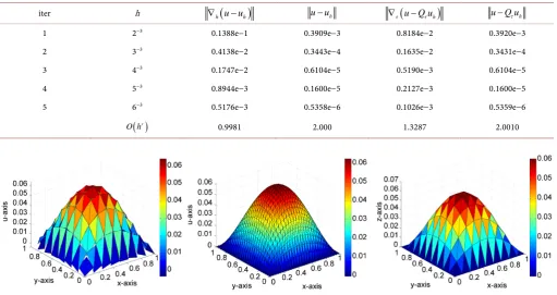
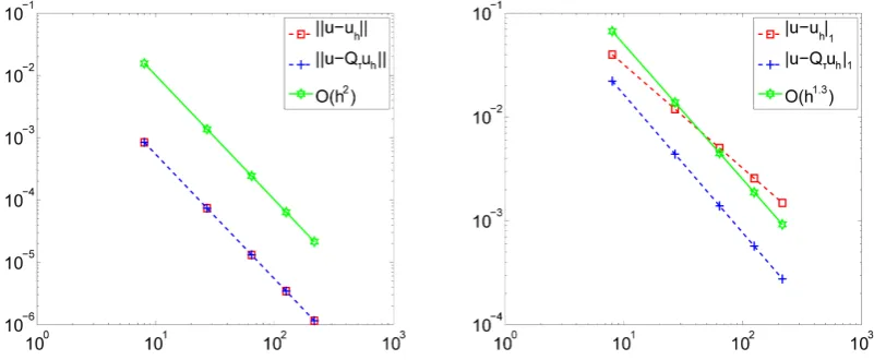
From Table 1 we observe that the L2_{-projection to the existing numerical approxi-} mation uh reduced the error estimates in L2 norm and in H1 norm. In L2 norm the convergence rate of u−Q uτ h is similar to the convergence rate of u−uh which is the same as the theoretical result (19). The convergence rate of u−Q uτ h1 is about 33% faster than the convergence rate of u−uh1 in H1 norm (see Figure 2). The surface plots of Q uτ h in coarse meshes and uh in fine meshes are shown in Figure 1. The numerical example 1 clearly supports the theoretical result and confirms the superconvergence of NCFEM for the second-order elliptic problem.

Example 2. Let the domain Ω =

[ ] [ ]

0,1× 0,1 and let the analytical solution be given

as

(

1

)

cos 1.5π .

(

)

u=x −x y y

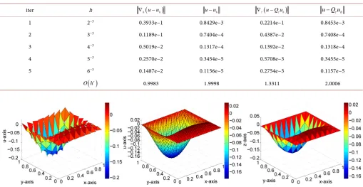
From Table 2, we can see that the numerical example 2 supports the theoretical result (15). See Figure 3, when 3

3

h= − and τ=3−2, we can project 32 fine triangle

elements onto one coarse triangle element. Thus, as n increases, we can project 2

n

[image:7.595.44.556.402.673.2]

more fine triangle elements to one coarse triangle element in which the process of refining elements produces better error estimates. The L2_{-projection to the existing} numerical approximation uh produced some superconvergence in H1 norm and did not affect the convergence rate in L2_{norm (see}_{Figure 4}_{). The numerical example 2 also}

Table 1. Numerical error approximation results using NCFEM in Example 1, u=x

(

1−x y

) (

1−y

)

.

iter h ∇h

(

u u− h

)

u u− h ∇τ

(

u Q u− τ h

)

u Q u− τ h

1 2−3 _0.1388e−1 _0.3909e−3 _0.8184e−2 _0.3920e−3

2 3−3 _0.4138e−2 _0.3443e−4 _0.1635e−2 _0.3431e−4

3 4−3 _0.1747e−2 _0.6104e−5 _0.5190e−3 _0.6104e−5

4 5−3 _0.8944e−3 _0.1600e−5 _0.2127e−3 _0.1600e−5

5 6−3 _0.5176e−3 _0.5358e−6 _0.1026e−3 _0.5359e−6

( )

r

O h 0.9981 2.000 1.3287 2.0010

Figure 1. Surface plots of approximation using NCFEM in Example 1, u=x

(

1−x y

) (

1−y

)

. (L): Surface plot of u_h when 3

2

h= − . (M): Surface of plot of uh when

3

h= − . (R): Surface plot of Q u_τ _h when 2

(8)

[image:8.595.141.551.68.237.2]

Figure 2. Error convergence rates using NCFEM in Example 1, u=x

(

1−x y

) (

1−y

)

. (L): L2 norm error; (R):

1

[image:8.595.43.553.303.566.2]

H norm error.

Table 2. Numerical error approximation results using NCFEM in Example 2, u=x

(

1−x y

)

cos 1.5

(

π .y

)

iter h ∇h(u−uh) u−uh ∇τ(u−Q uτ h) u Q u− τ h

1 2−3 _0.3933e−1 _0.8429e−3 _0.2214e−1 _0.8453e−3

2 3−3 _0.1189e−1 _0.7404e−4 _0.4387e−2 _0.7408e−4

3 4−3 _0.5019e−2 _0.1317e−4 _0.1392e−2 _0.1318e−4

4 5−3 _0.2570e−2 _0.3454e−5 _0.5708e−3 _0.3455e−5

5 6−3 _0.1487e−2 _0.1156e−5 _0.2754e−3 _0.1157e−5

( )

r

O h 0.9983 1.9998 1.3311 2.0006

Figure 3. Surface plots of approximation using NCFEM in Example 2, u=x

(

1−x y

)

cos 1.5

(

π .y

)

(L): Surface plot of u_h when 3

2

h= − .

(M): Surface of plot of uh when

3

h= − . (R): Surface plot of Q u_τ _h when 2

3 τ₌ − _.

supports the theoretical result and confirms the superconvergence of NCFEM for the second-order elliptic problem.

5. Conclusion

The L2_{-projection to the existing numerical approximation} h

u produced some super-

(9)

[image:9.595.149.550.74.239.2]

Figure 4. Error convergence rates using NCFEM in Example 2, u=x

(

1−x y

)

cos 1.5

(

π .y

)

(L): L2 norm error; (R): H1 norm error.

rate in L2_{norm. With the numerical experiments we can conclusively support the} theoretical result and confirm the superconvergence of NCFEM for second-order elliptic problems by L2_{-projection method.}

Acknowledgements

We thank the Editor and the peer-reviewers for their comments. Research of Anna Harris is funded by the National Science Foundation Historical Black Colleges and Universities Undergraduate Program Research Initiative Award grant (#1505119). This support is greatly appreciated.

References

[1] Croouzeix, M. and Raviart, P.A. (1973) Conforming and Nonconforming Finite Element Methods for Solving the Stationary Stokes Equations. R.A.I.R.O. R, 3, 33-76.

[2] Douglas Jr, J., Santos, J.E., Sheen, D. and Ye, X. (1999) Nonconforming Galerkin Methods Based on Quadrilateral Elements for Second Order Elliptic Problems. Mathematical

Model-ling and Numerical Analysis, 33, 747-770. https:/doi.org/10.1051/m2an:1999161

[3] Girault, V. and Raviart, P.A. (1986) Finite Element Methods for the Navier-Stokes Equa-tions: Theory and Algorithms. Springer, Berlin. https:/doi.org/10.1007/978-3-642-61623-5

[4] Wang, J. (2000) A Superconvergence Analysis for Finite Element Solutions by the Least- Square Surface Fitting on Irregular Meshes for Smooth Problems. Journal of Mathematical

Study, 33, 229-243.

[5] Ciarlet, P.G. (1978) The Finite Element Method for Elliptic Problems. North-Holland, New York.

[6] Ye, X. (2002) Superconvergence of Nonconforming Finite Element Method for the Stokes Equation. Numer. Method for PDE, 18, 143-154. https:/doi.org/10.1002/num.1036

(10)

Submit or recommend next manuscript to SCIRP and we will provide best service for you:

Accepting pre-submission inquiries through Email, Facebook, LinkedIn, Twitter, etc. A wide selection of journals (inclusive of 9 subjects, more than 200 journals)

Providing 24-hour high-quality service User-friendly online submission system Fair and swift peer-review system

Efficient typesetting and proofreading procedure

Display of the result of downloads and visits, as well as the number of cited articles Maximum dissemination of your research work