A new method for approximating vector autoregressive processes by finite state Markov chains

Munich Personal RePEc Archive

A new method for approximating vector

autoregressive processes by finite-state

Markov chains

Gospodinov, Nikolay and Lkhagvasuren, Damba

Concordia University, CIREQ

8 June 2011

A New Method for Approximating Vector

Autoregressive Processes by Finite-State

Markov Chains

Nikolay Gospodinov

Concordia University and CIREQ

Damba Lkhagvasuren

Concordia University and CIREQ

September 14, 2011

Abstract

This paper proposes a new method for approximating vector autoregressions by a finite-state Markov chain. The method is more robust to the number of discrete values and tends to outperform the existing methods over a wide range of the parameter space, especially for highly persistent vector autoregressions with roots near the unit circle.

Keywords: Markov Chain, Vector Autoregressive Processes, Functional Equation, Numerical Methods, Moment Matching

JEL Codes: C15, C60

1

Introduction

The finite-state Markov chain approximation methods developed by Tauchen (1986a) and

Tauchen and Hussey (1991) are widely used in solving functional equations where the state

variables follow autoregressive processes. Nonlinear dynamic macroeconomic and asset

pric-ing models often imply a set of integral equations (moment conditions) that do not admit

explicit solutions. Discrete-valued approximations prove to be an effective tool for reducing

the complexity of the problem. Also, there is a renewed interest in these methods for

gener-ating simulation data from nonlinear dynamic models in evalugener-ating the sampling properties

of generalized method of moments estimators (Tauchen, 1986b; Hansen, Heaton and Yaron,

1996; Stock and Wright, 2000; among others). The Markov-chain approximation methods

choose discrete values for the state variables and construct transition probabilities such that

the characteristics of the generated process mimic those of the underlying process. However,

bothTauchen (1986a) andTauchen and Hussey (1991) point out that these methods do not

perform well for highly persistent autoregressive (AR) processes or processes with

charac-teristic roots close to unity. Although these methods can generate a better approximation

at the cost of a finer state space, that type of approach is not always feasible.

The poor approximation of the methods by Tauchen (1986a) and Tauchen and Hussey

(1991) for strongly autocorrelated processes has spurred a renewed research interest given

the prevalence of highly persistent shocks in dynamic macroeconomic models. Rouwenhorst

(1995) proposes a Markov-chain approximation of an AR(1) process constructed by

target-ing its first two conditional moments. Some recent advances in the literature on

Markov-chain approximation methods includeAdda and Cooper (2003),Floden(2008) andKopecky

and Suen (2010). While these methods provide substantial improvements in approximating

highly persistent univariate AR(1) processes, their extension to vector autoregressive (VAR)

processes (as well as to higher-order autoregressive processes), which is of great practical

interest to macroeconomists, is not readily available and possibly highly non-trivial. As a

re-searchers for approximating multivariate processes by finite-state Markov chains. The only

alternative method that is available for approximating multivariate processes is the method

proposed by Galindev and Lkhagvasuren (2010). However, this method is developed for

a particular class of multivariate autoregressive processes: correlated AR(1) shocks, i.e., a

set of AR(1) shocks whose innovation terms are correlated with each other. Although this

method can be applied to vector autoregressions by decomposing the latter into a set of

interdependent AR(1) shocks, the state space generated by the method is not finite, except

for the special case of equally-persistent underlying shocks. Therefore, to the best of our

knowledge, a general method for approximating VAR processes by a finite-state Markov

chain with appealing approximation properties over the whole parameter region of interest

(including highly persistent parameterizations) is not yet available in the literature.

This paper fills this gap and proposes a new method for approximating vector

autoregres-sions (and higher-order scalar autoregressive processes) by a finite-state Markov chain. The

main idea behind this method is to construct the Markov chain by targeting conditional

mo-ments of the underlying continuous process as in Rouwenhorst (1995), rather than directly

calculating the transition probabilities using the distribution of the continuous process as in

the existing methods. In this respect, we give our method a moment-matching interpretation.

More specifically, we express the Markov-chain transitional probabilities as the solution of a

nonparametric (empirical likelihood) problem subject to moment restrictions. To target the

conditional moments in constructing the Markov chain, we use key elements of the Markov

chains generated by the methods of Tauchen (1986a) and Rouwenhorst (1995). Therefore,

the new method extends the methods of Tauchen (1986a) and Tauchen and Hussey (1991)

to highly persistent cases and Rouwenhorst (1995) and Kopecky and Suen (2010) to vector

cases, while still maintaining a finite number of states.

The new method yields accurate approximations without relying on a large number of

grid points for the state variables. In particular, the method extends the finite-state Markov

of the proposed method arise when the characteristic roots of the underlying process are

close to unity, it tends to outperform (in terms of bias and variance) the existing methods

even when the persistence is moderate or low. Finally, the method can be readily adapted

to accommodate other important features of the conditional distribution of the

continuous-valued process.

The rest of the paper is organized as follows. Section 2 introduces the continuous- and

discrete-valued versions of the multivariate model and the main notation. Section3 reviews

the existing approximation methods and demonstrates that they fail to deliver a reasonable

approximation as the roots of the continuous-valued process approach the unit circle. The

reason for this is that the existing methods calculate transition probabilities defined over

discrete grids using continuous probability density functions. Therefore, the quality of the

approximation deteriorates sharply when the standard deviation of the error terms becomes

comparable to or smaller than the distance between the grid points. Our new approximation

method is introduced in Section 4. We show that the new method matches the first two

conditional moments of the underlying process and describe the construction of the transition

probability matrix and the Markov chain. Section5 investigates the numerical properties of

the method in a bivariate VAR(1) process with a varying degree of persistence. Section 6

concludes. MATLAB codes for implementing the method are available from the authors upon

request. The proofs and some additional theoretical results are presented in Appendices A

and B.

2

Model

In this section we present the underlying continuous-valued vector autoregressive process

and introduce the main structure and notation for the finite-state Markov chain used for

2.1

Continuous VAR process

Let yt be an (M ×1) vector containing the values that variables, y1, y2,· · · , yM, assume at

date t. We consider the following vector autoregressive (VAR) process:

y_t=Ayt−1+εεεt, (1)

where A is an (M ×M) matrix with roots that lie strictly outside (although arbitrarily

close to) the unit circle and the (M ×1) vector εεεt is i.i.d N(0,Ω), where Ω is a diagonal

matrix. Extending the analysis to a non-diagonal Ω is relatively straightforward and is

discussed later in the paper.1 _{Our focus on the zero-mean, first-order VAR is primarily}

driven by expositional and notational simplicity and deterministic terms as well as

higher-order dynamics can be easily incorporated at the expense of additional notation. Let Σ

denote the unconditional covariance matrix of the processy. Then, it is the case that

Σ =AΣA′+ Ω. (2)

Let ai,j denote the row i, column j element of the matrix A. Also, let ωi and σi denote,

respectively, the square roots of thei-th diagonal elements of Ω and Σ fori_{∈ {}1,2,_{· · ·}, M_}.

2.2

Finite-state Markov chain

Let ˜yt denote the finite-state Markov chain that approximates yt in (1). Each component

˜

yi,t takes on one of the Ni discrete values denoted by ¯y(1)i ,y¯

(2)

i ,· · · ,y¯

(Ni)

i . Therefore, at each

point in time, the entire system will be in one of theN∗ _=N

1×N2× · · · ×NM states. Let

1_{Results for non-Gaussian errors, that target also the conditional skewness and kurtosis of the underlying}

¯

y(1)_,y¯(2)_{,· · · ,y¯}(N∗₎

label theseN∗ _{states and Π denote theN}∗_×N∗ _{transition matrix whose}

[row j, column k] element πj,k measures the probability that in the next period the system

will be in state k conditional on the current statej.

Our goal is to construct a finite number of grid points for each element of ˜yt and to

calculate the associated transition probability matrix Π so that the characteristics of the

generated process closely mimic those of the underlying process y.

Define

hi(j, l) = Pr(˜yi,t = ¯yi(l)|y˜t−1 = ¯y(j)) (3)

for i = 1,2,_{· · ·} , M, l = 1,2,_{· · ·} , Ni and j = 1,2,· · · , N∗. For any i, let Li be an

integer-valued function such that ˜yi = ¯y(L i(j))

i when the system is in state j. Given these functions,

the transition probability πj,k is given by the product of the individual transition

probabili-ties:

πj,k = M

Y

i=1

hi(j, Li(k)). (4)

This means that, for each pair (i, j), we need to construct Ni transition probabilities

Hi(j) ={hi(j,1), hi(j,2),· · · , hi(j, Ni)} (5)

over the grid points ¯y(1)_i ,y¯(2)_i ,· · · ,y¯(Ni)

i . Since, for each (i, j),

PNi

l=1hi(j, l) = 1, Hi(j) can be

considered as a probability mass distribution defined over the discrete values ¯y_i(1), ¯y(2)_i , _{· · ·},

¯

y(Ni) i .

The problem of determining the probability weights associated with this probability mass

distribution can be expressed as a nonparametric likelihood problem. In particular, the

nonparametric (or empirical) likelihood estimate of the transition probability matrix can be

obtained as the solution to the constrained maximization problem:

max

hi(j,l)∈[0,1]

M X i=1 N∗ X j=1 Ni X l=1

subject to the constraint

Ni

X

l=1

hi(j, l) = 1 for i= 1,· · · , M. (7)

To avoid trivial solutions, this optimization problem needs to be augmented with

addi-tional restrictions that best describe the statistical properties of model (1) for yt. These

restrictions typically take the form of conditional moments. Let

µi(j) =ai,1y¯1(L1(j))+ai,2y¯2(L2(j))+· · ·+ai,My¯(L M(j))

M (8)

for any i and j, denote the expected value of process yi,t+1, conditional on yt= ¯y(j). Then,

it seems natural to impose the restriction

Ni

X

l=1

hi(j, l)¯yi(l) =µi(j) (9)

for i = 1,_{· · ·} , M and j = 1,_{· · ·} , N∗ _{which requires that the Markov chain adequately}

approximates the conditional mean of the continuous-valued process y_t. The new method

that we propose below targets also the second conditional moment of the process yt by

imposing the additional restriction

Ni

X

l=1

hi(j, l)(¯yi(l)−µi(j))2 =ωi2 (10)

for i= 1,· · · , M and j = 1,· · · , N∗_.

3

Existing Methods

Before outlining the new method, we first discuss the disadvantages of the existing

finite-state methods for approximating vector autoregressions. We consider the method proposed

byTauchen(1986a) as a representative of these methods. The main reason is that, according

underlying process than its version inTauchen and Hussey(1991). Moreover, these existing

methods share the common feature that for calculating the transition probabilities defined

over discrete grids, they use continuous probability distribution functions. Finally, as argued

in the introduction, the finite-state extension of the recently proposed methods for improving

the Markov chain approximation in near-nonstationary region to multivariate processes is

not readily available.

The construction of the transition probabilities and the Markov chain for Tauchen’s

(1986a) method can be described as follows. For eachi,Tauchen(1986a) chooses equispaced

grid points over the interval [₋mσi, mσi] for some m >0.2 Specifically, for each i, the grid

points are chosen according to the following rule:

¯

y_i(l) =−mσi+ (l−1)△i, (11)

where_△i = 2mσi/(Ni−1) andl= 1,2,· · · , Ni. Note that△i measures the distance between

two consecutive nodes of ˜yi.

Given the above grid points, consider the following partition of the real line for each i:

C_i(1) =]−∞,y¯(1)_i +△i/2],Ci(Ni)=]¯y

(Ni)

i −△i/2,∞[, andCi(l) =]¯y

(l)

i −△i/2,y¯i(l)+△i/2],where

l = 2,3,· · ·, Ni−1. Tauchen (1986a) calculates the transition probabilities as

hi(j, l) = Pr

µi(j) +εi ∈Ci(l)

. (12)

Denoting the cumulative distribution function of the standard normal variable εi/ωi by Φi,

equation (12) can be rewritten as

hi(j, l) =

               Φi ¯

yi(1)−µi(j)+△i/2 ωi

if l = 1,

1₋Φi

¯

y(iNi)−µi(j)−△i/2 ωi

if l =Ni,

Φi

¯

yi(l)−µi(j)+△i/2 ωi

−Φi

¯

yi(l)−µi(j)−△i/2 ωi

otherwise.

(13)

According to Tauchen (1986a), the rationale for equations (8) and (12) is that if the

par-titioning C_i(1), C_i(2),_{· · ·} , C_i(M) is reasonably fine, then the conditional distribution of ˜yi,t

given state j at time t₋1 will approximate closely (in the sense of weak convergence) the

conditional distribution ofyi,t given yi,t−1 =µi(j).

Given the finite-state Markov chain ˜yt, let

˜

εεεt= ˜yt−Ay˜t−1, (14)

˜

Ω be the covariance matrix of ˜εεε and ˜ωi denote the square root of the i-th diagonal element

of this matrix. Since the conditional probabilities for this Markov chain are obtained by

centering the density ofεεεover Ay˜t−1, we have

E(˜yt|y˜t−1,y˜t−2,· · ·) =Ay˜t−1, (15)

and

E(˜εεεt) = E{E[(˜yt−Ay˜t−1)|y˜t−1,y˜t−2,· · ·]}= 0M. (16)

This implies, by the law of iterated expectations, that ˜εεεt is uncorrelated with ˜yt−s for

s = 1,2,_{· · ·}. However, the conditional covariance matrix of ˜εεεt, Var(˜εεεt|y˜t−1,y˜t−2,· · ·),

de-pends on ˜y_t−1 and thus, ˜εεεt and ˜yt−1 are dependent (Anderson, 1989). This clearly suggests

that targeting the second conditional moment will improve the quality of the Markov-chain

approximation and it serves as a main motivation for the new method proposed in this paper.

We now show that calculating the transition probabilities using the continuous

distribu-tion funcdistribu-tions does not always deliver meaningful approximadistribu-tions.

Proposition 1. Let ω˜2

i denote the conditional variance of˜εεεin equation (14), where y˜t is the

finite-state Markov chain constructed using the Tauchen’s (1986a) method . Then, for any

set of integers (N1, N2,· · · , NM) and any arbitrarily small positive number ǫ, there always

exists a vector autoregressive process for which ω˜2

Proof. See Appendix A.

Proposition 1 is an extension of the results in Galindev and Lkhagvasuren (2010). The

main implication of the result in Proposition1is that Tauchen’s (1986a) method will fail to

approximate the variability in y_t as one or more of the roots of the underlying

continuous-valued VAR process y_t approach the unit circle. This problem arises because most of the

existing approximation methods, including the method byTauchen (1986a), target only the

first conditional moment of the continuous-valued process yt.

A few remarks on some alternative approximation methods may seem warranted. Tauchen

and Hussey (1991) modify the method of Tauchen (1986a) by choosing the grid points

ac-cording to the Gaussian quadrature rule. However, Floden (2008) demonstrates that for a

wide range of parameters,Tauchen’s (1986a) method is more robust than the one inTauchen

and Hussey(1991). Floden(2008) uses an alternative weighting function to improve the

per-formance of the method inTauchen and Hussey(1991). However, some gains occur only over

a limited range of the parameters of the underlying process. In fact, Galindev and

Lkhagva-suren(2010) show that outside of the range considered by Floden(2008), his version fails to

generate any time varying Markov chain and thus is less robust than the method byTauchen

(1986a).

Despite some numerical and methodological differences across the existing Markov-chain

approximations, all these methods suffer from the same problem as inTauchen(1986a) since

they calculate the transition matrices using distribution functions centered around the first

conditional moment. In other words, regardless of the way the grid points are constructed,

there is a non-zero distance between any two grid points and thus one can directly extend

4

New Method

Having demonstrated the main shortcoming of the existing methods, we now propose an

alternative method for approximating a VAR process by a finite-state Markov chain.

4.1

Main idea

Unlike the existing finite-state methods for a multivariate process, which calculate the

transition probabilities using the conditional distribution function of yt, the new method

chooses the transition probabilities by targeting the key conditional moments ofyt.

Specifi-cally, it approximates the underlying process by targeting the 2M ×N∗ _{moment conditions}

given by equations (9) and (10). This means that the method chooses the grid points

{y¯(1)_i ,y¯_i(2),_{· · ·} ,y¯(Ni)

i }Mi=1 and the associated probability mass functions {Hi(1), Hi(2), · · ·,

Hi(N∗)}Mi=1 so that, for all i and j, the mean and the variance of distribution Hi(j) target,

respectively, µi(j) and ω2i.

The grid points and the probability mass functions are constructed using the method

of Rouwenhorst (1995). This particular choice of grid points and transition probabilities

generates a Markov chain which perfectly matches the conditional mean and conditional

variance of the underlying scalar AR(1) process.3 _{While incorporating information about the}

conditional variance is expected to deliver efficiency gains compared to Tauchen’s (1986a)

method over the whole permissible parameter range, we also show that this method has

some appealing properties when the underlying AR(1) process is highly persistent or near

unit root.

Although the method developed by Rouwenhorst (1995) tends to perform well in

ap-3_{In particular, for an AR(1) process y}

t = ρyt₋₁+εt,where |ρ| < 1, εt is i.i.d. N(0,(1−ρ2)σ2) with

σ2 _{= Var(y}

t), it can be shown that E(˜yt) = 0, Var(˜yt) =σ2 and Corr(˜yt,y˜t₋₁) =ρas well as E(˜yt|y˜t₋₁=

¯

y(k)_{) =ρy¯}(k)_{and Var(˜y}

t|y˜t₋₁= ¯y(k)) = (1−ρ2)σ2. One important feature of this result is that the persistence

proximating highly persistent scalar autoregressive processes,4 _{it is not readily applicable to}

the vector case. As pointed out in the introduction, the method by Galindev and

Lkhag-vasuren (2010) is tailored for approximating correlated AR(1) shocks and does not deliver

a finite-state space when adapted for approximating vector autoregressions.5 _{By contrast,}

the new method developed in this paper delivers a finite-state approximation regardless of

the degree of persistence of the different components of y while using only M state

vari-ables (i.e., ˜y1,y˜2, ...,y˜M). This could potentially offer substantial computational gains when

solving functional equations.

4.2

Markov chain construction

We use the following procedure to construct the Markov chain ˜y:

1. For each i, set n=Ni, s=σi and ρ=

p

1−ω2

i/σ2i.

2. FollowingRouwenhorst(1995), constructndiscrete values{y¯(1)_i ,y¯(2)_i ,· · · ,y¯_i(n)}that are

computed as

¯

y_i(k) =₋s√n₋1 + √2s

n−1(k−1) (17)

for k= 1,2,_{· · ·} , n, and let these be the grid points of ˜yi.

3. Construct the probability transition matrix of an n-state (scalar) Markov process with

persistenceρ. Let P(n)_{(ρ) denote this matrix. When n= 2, the probability transition}

matrix is given by

P(2)(ρ) =



 

1+ρ

2 1−ρ

2

1−ρ

2 1+ρ

2





. (18)

4_{See, for example, Galindev and Lkhagvasuren (2010) and Kopecky and Suen (2010) for a numerical}

comparison of the method of Rouwenhorst (1995) with some commonly-used existing methods including those ofTauchen(1986a) andTauchen and Hussey(1991).

5_{In order to approximate an M-variate process y}

t given by equation (1), in general, the method by

For higher values ofn, the transition probability matrix is constructed recursively using

the elements of matrix P(2)_{(ρ) (for details, see Rouwenhorst (1995)). Let p}(n)

k,l(ρ), the

rowk, columnl element ofP(n)_{(ρ), be the probability that then-state process switches}

from ¯y_i(k) to ¯y_i(l). Consequently, the k-th row of the matrix P(n)_{(ρ) is given by}

p_k(n)(ρ) ={p_k,(n₁)(ρ), p_k,(n₂)(ρ),· · · , p_k,n(n)(ρ)}. (19)

Since Pn

l=1p (n)

k,l(ρ) = 1, this row can be interpreted as a probability mass function

associated with the nodes _{y¯_i(1),y¯_i(2),_{· · ·} ,y¯_i(n)_}. Note that the mean and the variance

of the probability mass distribution p(_kn)(ρ) are, respectively, ρy¯_i(k) and ω2

i.

4. For each j ∈ {1,2,· · · , N∗_{}, we consider the following four distinct cases:}

(a) If µi(j)< ρy¯i(1), set

Hi(j)≡p(1n)(ρ). (20)

(b) If µi(j)> ρy¯i(n), set

Hi(j)≡p(nn)(ρ). (21)

In these two cases, the conditional variance ω2

i is matched while the conditional

mean attains the value closest to µi(j) given the grid points.

(c) If µi(j) =ρy¯i(k) for some k∈ {1,2,· · · , n}, set

Hi(j)≡p(_kn)(ρ). (22)

In this case, both the conditional mean µi(j) and conditional variance ω2i are

matched.6

(d) If any of the above three conditions is not met, there must be an integer k such

6_{This case includes the special sub-case σ}

i = ωi. Therefore, when ρ = p

1−ω2

i/σ2i = 0, set Hi(j) =

that 1 ≤ k ≤ n−1 and ρy¯_i(k) < µi(j) < ρy¯i(k+1). Then, consider the following

mixture distribution defined over{y¯(1)_i ,y¯(2)_i ,· · · ,y¯_i(n)} for some 0< λ <1:

˜

p(_kn)(ρ) = λp(_kn)(ρ) + (1₋λ)p(_kn₊₁) (ρ), (23)

where

λ = ρy¯

(k+1)

i −µi(j)

ρy¯_i(k+1)−ρy¯_i(k). (24)

The mean and variance of this new probability mass distribution are, respectively,

˜

µk(ρ) = µi(j) (25)

and

˜

ω_k2(ρ) = (1₋ρ2)s2+ρ2λ(1₋λ)y¯(_ik+1)₋y¯(_ik)2. (26)

Since 0 < λ < 1, ˜ω2

k(ρ) > (1−ρ2)s2 = ωi2.7 This means that although the

mean of the mixture distribution ˜p(_kn)(ρ) hits its target µi(j), the variance of the

distribution is greater than our target ω2

i. It is easy to observe that ˜ωk2(ρ) goes

down asρincreases. Therefore, we repeat the calculations in Steps 3 and 4(d) for

higher values ofρ and choose the one which minimizes the distance _|ω˜2

k(ρ)−ωi2|.

Letρ∗ _{be the value ofρ found in such a manner. Then, set}

Hi(j)≡p˜k(n)(ρ∗). (27)

In this case, the conditional mean µi(j) is matched, but the conditional variance

achieves the best possible value given the grid points.

7_{Note that sinceρ <1 andλ(1}

Repeating this procedure for i = 1,2,· · · , M, we construct the grid points {y¯_i(1), y¯(2)_i ,

· · · ,y¯(Ni)

i }Mi=1and the probability mass functions{Hi(1),Hi(2),· · ·,Hi(N∗)}Mi=1. Given these

probability mass functions, we construct the transition probability matrix of the Markov

chain ˜y, Π, using equations(4) and (5). The asymptotic validity of the method is discussed

in Appendix B.

While the procedure above is developed under the assumption of a diagonal covariance

matrix Ω, the proposed method can be easily extended to the case of a non-diagonal

covari-ance matrix. Suppose now that the underlying continuous-valued process follows

xt=b+Bxt−1+ηt, (28)

where ηt is i.i.d (0,Ψ) and Ψ is a non-diagonal matrix.8 LetG be a lower triangular matrix

such that Ω =GΨG−1 _{is a diagonal matrix. Define the transformations (Tauchen, 1986b),}

xt →G[yt−(IM −B)−1b], (29)

B →A=GBG−1, (30)

and

ηt→Gεt. (31)

Then, we have the same model as in equation (1). After computing the discrete

Markov-chain approximation for this modified model, we reverse the transformations above in order

to obtain the discrete process corresponding to equation (28).

Furthermore, since any stationary AR(p) process can be expressed in a companion form

as a VAR(1) process, our method effectively extends the method by Rouwenhorst (1995)

to higher-order scalar autoregressive processes. Another appealing feature of our method is

8_{See also Terry and Knotek II (2011), who extend Tauchen (1986a) to processes with a non-diagonal}

its flexibility which allows us to deal with possibly nonlinear VAR processes and targeting

additional moments of the conditional distribution such as skewness and kurtosis.

Below we examine numerically how well the method works in terms of approximating

autoregressive processes for various degrees of persistence of the discrete space. We show that

the new method outperforms the method by Tauchen (1986a), especially for the processes

whose characteristic roots are close to one.

5

Numerical Evaluation

For our main numerical evaluation, we consider the bivariate VAR(1) case (M = 2) with

εεεt∼i.i.d N

      0 0   ,   

0.1 0

0 0.1

      (32)

and A=AK

0 , where

A0 =



 

0.995619 0.005335

0.003557 0.992063





 (33)

and K is a positive integer set to 1, 10 and 100.9 _{It is straightforward to see that higher}

values ofK imply lower persistence. As inTauchen (1986a), we choose nine grid points for

each component: ˜N =N1 =N2 = 9. We also consider another case in which the state space

is much finer: ˜N = 19.

9_{The matrixA}

0 is chosen for comparison purposes: whenK= 100,

A=A1000 =

0.7 0.3 0.2 0.5

5.1

The accuracy of the approximation

Let {y˜t}τt=1 denote simulated time series either from the Markov chain approximation by

Tauchen (1986a) or the method proposed in this paper. The accuracy of the two

approx-imations can then be examined by estimating the key parameters of the initial process in

equation (1). The parameters of interest are the unconditional variances of y1 and y2

(de-noted byσ2

1 andσ22), the cross-correlation coefficient between y1 and y2, and the persistence

measures 1₋ξ1 and 1−ξ2, where ξ1 and ξ2 are the two roots (eigenvalues) of matrix A.

As in Tauchen (1986a) andTauchen and Hussey (1991), the simulated counterpart ofA, ˆA,

is obtained by fitting the linear autoregressive model in equation (1) to _{y˜t}τt=1. The

sum-mary of the approximation accuracy is based on 1,000 Monte Carlo replications of length

τ = 2,000,000. Tables 1 and 2 report the root mean squared errors (RMSE) as well as the

biases and standard deviations of these parameters relative to their true values.

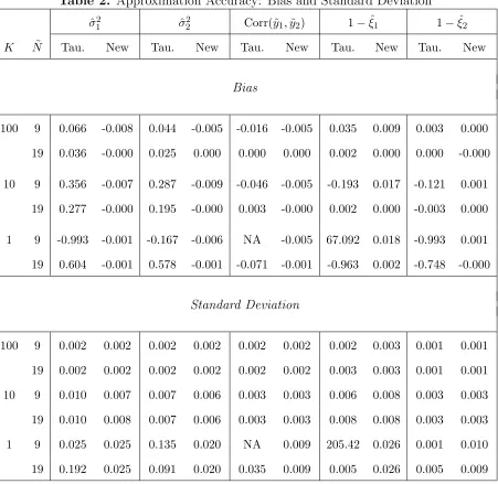
The results suggest that the new method dominates the method by Tauchen (1986a) in

terms of bias and RMSE for all parameters of interest across all degrees of persistence. For

example, for the least persistent case (K = 100), the relative bias for ˜N = 9 of the estimated

1₋ξ1, σ12 and σ22, using data generated by Tauchen’s (1986a) method, is 3.5%, 6.6% and

4.4%, respectively, whereas the corresponding biases for the new method are 0.9%, -0.8%

and -0.5%. For the moderate degree of persistence (K = 10), the biases for the method of

Tauchen (1986a) become -19.3%, 35.6% and 28.7%, while those of the new method remain

almost constant at 1.7%, -0.7% and -0.9%, respectively. However, the significant advantages

of our method become particularly striking for the high persistence case (K = 1). For

this degree of persistence, Tauchen’s (1986a) method fails to produce any time variation

in the approximate Markov chain process, which is consistent with our theoretical results

in Proposition 1. For example, the average probability of switching from the current state

to any other state (with ˜N = 9) is only 0.03% for the method by Tauchen (1986a). This

results in substantially large biases and inflated RMSEs for the parameters of interest. At

RMSEs. Increasing the number of grid points from 9 to 19 improves the performance of

Tauchen’s (1986a) method in the less persistent cases but its numerical properties in the

highly persistent case remain rather poor.

Kopecky and Suen(2010) prove that the invariant distribution of the Markov chain

con-structed by Rouwenhorst’s (1995) method is a binomial distribution. A direct consequence

of this result is that the invariant distribution of the Markov chain constructed by

Rouwen-horst’s (1995) method converges asymptotically (as the number of states goes to infinity) to

a normal distribution. This is not surprising because the method by Rouwenhorst (1995)

targets only the first two conditional moments of the underlying process. Therefore, it might

be instructive to see how our new method and Tauchen’s (1986a) method approximate the

higher-order moments (skewness and excess kurtosis) of the continuously-valued process.

The results (not reported here to conserve space) show that the higher-order moments of

the two methods do not differ much when the persistence is low. When persistence is high,

the new method outperforms (often substantially) Tauchen’s method by generating skewness

and excess kurtosis much closer to their true values. In highly persistent cases, the method

byTauchen(1986a) often fails to generate any variation in some of the components of ˜y (see

Proposition1) and thus their higher-order moments are not defined.

5.2

Conditional moments

The evaluation of the approximation accuracy in Tables 1 and 2 is based on unconditional

moments of the underlying and simulated processes. Potentially important information

about the quality of the approximation is also contained in the conditional moments. Hence,

it would be interesting also to report the first two moments, conditional on the state of the

process.

Given the constructed grid points and transition probabilities, the implied conditional

mean and variance are ˆµi(j) =PNil=1hi(j, l)¯yi(l)and ˆω2i(j) =

PNi

l=1hi(j, l)(¯yi(l)−µˆi(j))2,where

the targeted and the generated conditional moments can be measured by_|µˆi(j)−µi(j)| and

|ωˆ2

i(j)/ωi2−1|. To assess the overall accuracy of the conditional moments, we consider the

weighted averages of these distances across the N∗ _{states using the frequencies of each state}

as weights. The weights are constructed from a simulated process of length τ = 2,000,000.

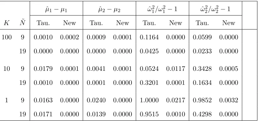
The results are presented in Table 3 and show that the new method performs extremely well

across all parameterizations. Again, this is not surprising since, by construction, this method

targets the first two conditional moments of the underlying process. More importantly, the

results show that calculating the transition probabilities using the conditional distribution, as

inTauchen (1986a), generates a substantial bias in the conditional moments. This numerical

finding also lends support to our theoretical result in Proposition 1.

6

Conclusion

This paper proposes a new method for approximating vector autoregressions by a

finite-state Markov chain. The main idea behind this method is to construct the Markov chain

by targeting a set of conditional moments of the underlying process rather than

calculat-ing the transition probabilities directly from an assumed distribution, centered around the

first conditional moment, as in the existing methods. The new method yields accurate

ap-proximations for a wide range of the parameter space, without relying on a large number

of grid points for the state variables. The improved approximation accuracy of the

pro-posed method is expected to have important quantitative implications for solving dynamic

A

Proof of Proposition 1

We establish the result in Proposition 1 for process i, we parameterize the high persistence

as local-to-unity (see Phillips, 1987, for example).

Let ˜y_T(n) = (˜y₁(n),y˜₂(n),· · ·,y˜(tn),· · · ,y˜

(n)

T ) be a realization of the n-state Markov chain of

lengthT approximated over ngrid points. In what follows, we keep nfixed and perform the

analysis as T → ∞. In the local-to-unity framework, the autoregressive parameter in the

AR process is reparameterized as a function ofT as

ρ= 1₋ c

T, (A.1)

wherec >0 is a fixed constant. This is an artificial statistical device in which the parameter

space is a shrinking neighborhood of one asT increases. This parameterization proves to be

a very convenient tool to study the properties of strongly dependent processes asT _{→ ∞}.

First note that using this reparameterization, the variance of the innovation for the

continuous-valued process can be expressed as

ω2 _{= (1−ρ}2_)σ2 ₌ 2cσ2

T − c2_σ2

T2 . (A.2)

For Tauchen’s (1986a) method, the probability that the process switches from state j

(cor-responding to grid point ¯y(j)_{) to any other state is given by}

1₋πj,j = 1−Pr

ε₋ cy¯

(j)

T ≤ 2_△ (A.3)

where πj,j is the j-th diagonal element of Π. As T → ∞, the persistence of the process

increases and 0<y¯(j)_{/T <2△ (for all j) with probability approaching one. Therefore,}

1−πj,j ≤1−Pr (|ε| ≤2△) = 2 1−Φ

2△

p

σ2_(1−ρ2₎

!!

<2 1−Φ 2△

√ T √

2cσ2

!!

and

1₋πj,j

ω2 <

21−Φ△

√ 2T σ√c

2cσ2_{/T −c}2_σ2_/T2 (A.5)

for all j. Since

Φ △

√

2T σ√c

!

→1 as T _{→ ∞}, (A.6)

by l’Hopital’s rule,

lim

T→∞

1₋πj,j

ω2 =

△

2σ3_c3/2_π1/2

1

(1/T3/2_−c/T5/2_{) exp(2c△}2 _{T /σ}2₎ = 0. (A.7)

Hence, since the limiting behavior of the conditional variance of the Markov-chain

approxi-mation is determined by the limiting behavior of 1−πj,j,

˜

ω2

ω2 →0 as T → ∞. (A.8)

This completes the proof of Proposition 1.

B

Asymptotic validity of the approximation method

Consider the following scalar continuous-valued AR(1) process y′ _{= ρy+ε (|ρ| < 1) with}

conditional density f(y′_{|y) and the function}

eg(y) =

Z

g(y′_)f(y′_{|y)dy, (B.1)}

where g(y) _∈ C0[a, b] and C0[a, b] denotes the space of continuous functions on [a, b] with

a < b and both a and b are finite. Assume that the support of f(y′_{|y) is a subset of}

[a, b]×[a, b] and f(y′_{|y) is jointly continuous in y}′ _{and y. Let ˜y denote the n-state}

transition probabilities π(_j,kn) = Pr(˜y′ _{= ¯y}(k)_{|y˜= ¯y}(j)_{). Let}

egn(y) = n

X

k=1

g(¯y(k))π_j,k(n). (B.2)

Following Tauchen and Hussey (1991), we need to show the uniform convergence result

sup

y∈[a,b]|

egn(y)−eg(y)| p

→0 (B.3)

as n_{→ ∞}.

The pointwise convergence of the conditional distribution of the Markov chain ˜y′ _given

˜

y= ¯y(j) _{to the conditional distribution ofy}′ _{giveny=µ(j) can be inferred from noting that}

the transition probability matrix for our method can be expressed in a polynomial form (see

Kopecky and Suen,2010) and by appealing to the Stone-Weierstrass approximation theorem.

Finally, the condition that egn(y) is uniformly bounded converts the pointwise convergence

into uniform convergence. As a result,egn(y) is equicontinuous which is a sufficient condition

for the uniform convergence result

sup

y∈[a,b]|

egn(y)−eg(y)| p

References

Adda, Jerome and Russel Cooper (2003).Dynamic Economics, MIT Press, Cambridge, MA.

Anderson, Theodore W. (1989). “Second-Order Moments of a Stationary Markov Chain

and Some Applications,” Technical Report No. 22, Department of Statistics, Stanford

University.

Fernandez-Villaverde, Jesus, Pablo Guerron-Quintana, Juan F. Rubio-Ramirez and Martin

Uribe (forthcoming). “Risk Matters: The Real Effects of Volatility Shocks,” American

Economic Review.

Floden, Martin (2008). “A Note on the Accuracy of Markov-Chain Approximations to Highly

Persistent AR(1) Processes,”Economics Letters, 99 (3): 516–520.

Galindev, Ragchaasuren and Damba Lkhagvasuren (2010). “Discretization of Highly

Per-sistent Correlated AR(1) Shocks,” Journal of Economic Dynamics and Control, 34 (7):

1260–1276.

Hansen, Lars Peter, John Heaton and Amir Yaron (1996). “Finite-Sample Properties of Some

Alternative GMM Estimators,”Journal of Business and Economic Statistics, 14 (3): 262–

280.

Kopecky, Karen A. and Richard M.H. Suen (2010). “Finite State Markov-Chain

Approxi-mations to Highly Persistent Processes,”Review of Economic Dynamics, 13 (3): 701–714.

Phillips, Peter C. B. (1987). “Towards a Unified Asymptotic Theory for Autoregression,”

Biometrika, 74 (4): 535–547.

Rouwenhorst, Geert K. (1995). “Asset Pricing Implications of Equilibrium Business Cycle

Models,” in Thomas Cooley, ed., “Structural Models of Wage and Employment Dynamics,”

Stock, James H. and Jonathan Wright (2000). “GMM with Weak Identification,”

Economet-rica, 68 (5): 1055–1096.

Tauchen, George (1986a). “Finite State Markov-Chain Approximations to Univariate and

Vector Autoregressions,”Economics Letters, 20 (2): 177–181.

Tauchen, George (1986b). “Statistical Properties of Generalized Method-of-Moments

Es-timators of Structural Parameters Obtained From Financial Market Data,” Journal of

Business and Economic Statistics, 4 (4): 397–416.

Tauchen, George and Robert Hussey (1991). “Quadrature-Based Methods for Obtaining

Approximate Solutions to Linear Asset Pricing Models,”Econometrica, 59 (2): 371–396.

Terry, Stephen J. and Edward S. Knotek II (2011). “Markov-Chain Approximations of Vector

Autoregressions: Application of General Multivariate-Normal Integration Techniques,”

Table 1. Approximation Accuracy: RMSE

ˆ

σ₁2 σˆ₂2 Corr(˜y1,y˜2) 1−ξˆ1 1−ξˆ2

K N˜ Tau. New Tau. New Tau. New Tau. New Tau. New

100 9 0.066 0.008 0.044 0.005 0.017 0.006 0.035 0.010 0.003 0.001

19 0.036 0.002 0.025 0.002 0.002 0.002 0.003 0.003 0.001 0.001

10 9 0.356 0.010 0.287 0.011 0.047 0.006 0.193 0.019 0.121 0.003

19 0.278 0.008 0.195 0.006 0.004 0.003 0.008 0.008 0.004 0.003

1 9 0.993 0.025 0.215 0.021 NA 0.010 216.099 0.032 0.993 0.010

19 0.634 0.025 0.585 0.020 0.079 0.009 0.963 0.026 0.748 0.010

Notes. This table reports the root mean squared error (RMSE) of the key parameters of

the bivariate VAR(1) model relative to their true values. (See Section 5for details). ”Tau.”

denotes the approximation obtained by the method of Tauchen (1986a) whereas ”New”

denotes the Markov chain approximation method developed in this paper. Higher values of

K imply less persistence. ˜N stands for the number of grid points used for each component

of y. ˆσ2

i denote the simulated unconditional variance of ˜yi where i ∈ {1,2}. Corr(˜y1,y˜2) is

the cross-correlation coefficient between ˜y1 and ˜y2. ˆξ1 and ˆξ2 are the eigenvalues of matrix

ˆ

A. NA indicates that, in some cases, there is no variation in ˜y1 and, therefore, ˆσ21 = 0 and

the correlation coefficient Corr(˜y1,y˜2) is not defined. The fact that the RMSE of ˆσ12 relative

to its true value is very close to 1 indicates that, for most of the Monte Carlo experiments,

Table 2. Approximation Accuracy: Bias and Standard Deviation

ˆ

σ₁2 ˆσ₂2 Corr(˜y1,y˜2) 1−ξˆ1 1−ξˆ2

K N˜ Tau. New Tau. New Tau. New Tau. New Tau. New

Bias

100 9 0.066 -0.008 0.044 -0.005 -0.016 -0.005 0.035 0.009 0.003 0.000

19 0.036 -0.000 0.025 0.000 0.000 0.000 0.002 0.000 0.000 -0.000

10 9 0.356 -0.007 0.287 -0.009 -0.046 -0.005 -0.193 0.017 -0.121 0.001

19 0.277 -0.000 0.195 -0.000 0.003 -0.000 0.002 0.000 -0.003 0.000

1 9 -0.993 -0.001 -0.167 -0.006 NA -0.005 67.092 0.018 -0.993 0.001

19 0.604 -0.001 0.578 -0.001 -0.071 -0.001 -0.963 0.002 -0.748 -0.000

Standard Deviation

100 9 0.002 0.002 0.002 0.002 0.002 0.002 0.002 0.003 0.001 0.001

19 0.002 0.002 0.002 0.002 0.002 0.002 0.003 0.003 0.001 0.001

10 9 0.010 0.007 0.007 0.006 0.003 0.003 0.006 0.008 0.003 0.003

19 0.010 0.008 0.007 0.006 0.003 0.003 0.008 0.008 0.003 0.003

1 9 0.025 0.025 0.135 0.020 NA 0.009 205.42 0.026 0.001 0.010

19 0.192 0.025 0.091 0.020 0.035 0.009 0.005 0.026 0.005 0.009

Notes. This table reports the bias and the standard deviation of the parameters relative to

their true values. For the bias, the numbers that are much smaller than 0.0005 (0.05%) in

Table 3. The Distance between Generated and True Conditional Moments

ˆ

µ1−µ1 µˆ2−µ2 ωˆ12/ω12−1 ωˆ22/ω22−1

K N˜ Tau. New Tau. New Tau. New Tau. New

100 9 0.0010 0.0002 0.0009 0.0001 0.1164 0.0000 0.0599 0.0000

19 0.0000 0.0000 0.0000 0.0000 0.0425 0.0000 0.0233 0.0000

10 9 0.0179 0.0001 0.0041 0.0001 0.0524 0.0117 0.3428 0.0005

19 0.0010 0.0000 0.0001 0.0000 0.3201 0.0001 0.1634 0.0000

1 9 0.0163 0.0000 0.0240 0.0000 1.0000 0.0217 0.9852 0.0032

19 0.0171 0.0000 0.0139 0.0000 0.9515 0.0010 0.4298 0.0000

Notes. This table reports the overall distance between generated and true conditional

mo-ments. Specifically, fori∈ {1,2}, the numbers in column ˆµi−µi, are the weighted average of

|µˆi(j)−µi(j)|which uses the frequencies of statesj = 1,2, ..., N∗ as weights. The frequencies

are constructed using a simulated process of length τ = 2,000,000. Similarly, the numbers

in column ˆω2

i/ω2i −1 for i ∈ {1,2} are the weighted average of |ωˆ2i(j)/ωi2 −1| which uses

the same frequencies as in columns ˆµi−µi. The numbers that are smaller than 0.00005 are