Munich Personal RePEc Archive
Reassessing the Evolution of World
Trade, 1870-1949
Klasing, Mariko and Milionis, Petros
June 2012
Reassessing the Evolution of World Trade, 1870-1949
Mariko J. Klasing
Petros Milionis
yCarleton University University of Groningen
June 2012
Abstract
The typical narrative regarding the evolution of world trade prior to World War II refers to a secular rise that started around 1870 and a subsequent collapse that began in 1914. This narrative, though, is based on measures of trade openness that do not fully take into account purchasing power di¤erences across countries, as in the literature non-PPP-adjusted trade data are typically denominated by PPP-non-PPP-adjusted GDP data. The present paper seeks to resolve this inconsistency by constructing new trade share estimates for 51 countries spanning the period from 1870 to 1949 by combining historical import and export data with non-PPP-adjusted GDP values that we estimate via the "short-cut" method. Our estimates indicate a much more pronounced rise and fall of world trade over this period with trade shares being on average 32% higher than previously documented and the world’s level of openness to trade in 1913 being comparable to that in 1974. In addition, performing a similar correction for purchasing power di¤erences in the context of standard gravity regressions for the 1870-1939 period we …nd that the existing literature has overestimated the importance of income movements during this period relative to tari¤s changes and the evolution of the gold standard.
Keywords: International Trade, Purchasing Power Di¤erences
JEL Classi…cation: F01, F15, N10, N70.
Department of Economics, Carleton University, 1125 Colonel By Drive, Ottawa, ON K1S 5B6, Canada; e-mail address: [email protected].
yDepartment of Economics, Econometrics & Finance, Faculty of Economics & Business, University of
1
Introduction
We live in a globalized world. Yet, to what extent is the recent globalization movement that the world has witnessed since the 1950s a singular experience? A precise answer to such a question requires a careful quanti…cation of how open the world economy was prior to World War II. The present paper is the …rst to attempt to consistently measure trade openness for a large number of countries during the period from 1870 to 1949. Based on that, we then seek to reassess the determinants of international economic integration, as it evolved over this period.
Our choice to focus on the eight decades prior to 1950 is neither accidental nor without precedent. In the recent years a growing number of international economists and economic historians has turned to the study of this period that comprises the years of World War I and II, the turbulent interwar era as well as the pre-war Belle Époche.1 Particularly this last period
-often referred to as the …rst globalization era- has attracted a lot of attention, as it very much resembles today’s world in terms of international trade as well as capital ‡ows.2
However, as with the study of any historical period, existing work that has attempted to assess and analyze the degree of openness of di¤erent economies and the world as a whole during the pre-World-War-II period has been constrained by the incompleteness of the available data. As a consequence, when measuring trade shares researchers were typically forced to combine nominal, namely non-PPP-adjusted, export and import data with real, namely PPP-adjusted, GDP values such as those of Maddison (2001).3;4 Trade shares calculated in this fashion, though,
are subject to systematic biases given the well-known fact that relative price di¤erences across countries vary systematically with the level of economic development.5
To avoid such biases in the present paper we construct trade shares for the largest-possible set of countries spanning the period from 1870 to 1949 based on non-PPP-adjusted GDP values. These values are estimated via the "short-cut" method, a method which enables the prediction of nominal from real income values and vice versa, as we explain in Section 2. Following this method, which was widely used at the time when internationally comparable national account data were more scarce, we can obtain estimates for non-PPP-adjusted GDP for the period of interest for 68 countries based on the PPP-adjusted GDP …gures of Maddison (2001). Given the available export and import data, this allows for the consistent measurement of trade shares for 51 countries.
To assess the quality of our estimated nominal income and implied trade share data, we 1See for example the work of O’Rourke and Williamson (1999), Estevadeordal, Frantz, and Taylor (2003),
Jacks, Meissner, and Novy (2010), Schularick and Solomou (2011) and the references therein.
2See for example the comparisons made by Krugman (1995) and Obstfeld and Taylor (2004).
3Following the language of the international comparison literature, we will often use the term "real" to refer
to PPP-adjusted measures and the term "nominal" to non-PPP-adjusted ones.
4Examples of cases were nominal trade data were combined with real income data can be found in
Estevade-ordal, Frantz, and Taylor (2003), Lopez-Cordova and Meissner (2003) and Jacks, Meissner, and Novy (2011).
compare them with the corresponding ones that we were able to obtain from existing historical sources for a small set of 16 countries for the years prior to 1949. For those limited cases, as we document in Sections 2 and 3, we …nd our estimated values to be remarkably close to the actual ones. Moreover, we also compare our non-PPP-adjusted GDP and trade share estimates with those obtained in the case where no correction for purchasing power di¤erences is made. This latter comparison reveals that, as one would expect, not correcting for such di¤erences leads to a substantial underestimation of trade shares for most countries.6
Having established the quality of our estimated trade shares, in Section 3, we then turn to discuss what they imply for the evolution of world trade prior to World War II. In this context we …rst document how overall both the expansion of international trade over the 1870-1913 period as well as its collapse between 1919 and 1939 was much more pronounced than what the existing literature has suggested. Speci…cally we …nd that trade shares during the period 1870-1949 were on average 32% higher than what previous research had established, implying that the extent of international trade during the height of the …rst globalization era was comparable to that observed during the mid 1970s. In addition, tracking the behavior of our trade share estimates across di¤erent regions of the globe, we observe di¤erent regional patterns with the Western European economies driving the pre-World-War-I trade expansion and these economies together with those of Latin America accounting for most of the subsequent retreat.
Extending our analysis beyond the discussion of global and regional trade patterns that prevailed prior to World War II, in Section 4 we also pursue a gravity approach to shed more light on the determinants of international trade ‡ows going back to 1870. In this respect we follow closely the work of Eichengreen and Irwin (1995), Irwin and Terviö (2002), Estevadeordal, Frantz, and Taylor (2003), Lopez-Cordova and Meissner (2003), Jacks, Meissner, and Novy (2010) and others who have employed gravity models to analyze historical bilateral trade ‡ows. Yet, in contrast to most existing contributions, we estimate our gravity speci…cation combining non-PPP-adjusted bilateral trade data with our estimated non-non-PPP-adjusted income data instead of PPP-adjusted ones.
Focusing on the role of income growth, tari¤s and the gold standard in in‡uencing trade ‡ows between countries, we consider their predictive power in the context of the gravity model and the relative importance of each in explaining the evolution of bilateral trade ‡ows over time. In this context we show how the common approach of employing PPP-adjusted GDP data instead of non-PPP-adjusted ones leads to a systematic overestimation of the e¤ect of income growth and an underestimation of that of tari¤s and the gold standard. Yet, as we demonstrate in a counterfactual analysis based on our gravity estimation results, pair-speci…c income movements still explain most of the observed growth in bilateral trade during the …rst globalization era. 6This is due to imports and exports being divided with PPP-adjusted income values that are higher than their
Contrary, though, during the interwar period the collapse of bilateral trade ‡ows was primarily the result of the global trend towards trade disintegration.
2
Estimating Nominal GDP
2.1
The "Short-Cut" Method
A correct calculation of historical trade shares based on nominal trade data requires a corre-sponding set of nominal, namely non-PPP-adjusted, GDP values. Such information, though, is currently only scarcely available. To avoid this data limitation problem, we employ the "short-cut" method in order to estimate nominal GDP in current prices for the largest possible set of countries and time-periods based on the available information on real, namely PPP-adjusted, GDP. This method has a long tradition in the literature on international comparison going back to the work of David (1972) and Kravis, Heston, and Summers (1978) and was recently revived by Prados de la Escosura (2000).7 Its rationale is to exploit the existence of a fundamental
structural relationship between nominal and real GDP in per capita terms, which is stable across countries and time.
The posited relationship arises from the basic fact that the ratio of nominal to real GDP per capita in a given country at any point in time - when each is expressed relative to a base country-re‡ects the country’s general price level vis-à-vis that of the base country. This in turn depends on the relative price levels of the country’s traded and non traded goods. The former tends to approach unity with international competition, while the latter depends on the country’s relative income level, as the Balassa-Samuelson theorem predicts.8 As a result, the overall price level of
a country - and so its ratio of nominal to real per capita GDP - should vary with the country’s level of development and degree of openness. This implies the existence of a direct relationship between relative nominal and real GDP per capita.
Denoting with yP P P
i the level of PPP-adjusted GDP per capita of a country i relative to
the base country -which for the context of our analysis we take to be the United States- and
yinon P P P the corresponding level of non-PPP-adjusted GDP per capita, the "short-cut" method
posits that,
yinon P P P =f(yP P Pi ; P Ii); (1)
with P Ii being a measure of country i’s degree of price isolation from the rest of the world.9
7Kravis, Heston, and Summers (1978), for example, employed this method to predict PPP-adjusted GDP per
capita for more than a 100 countries using information from a sample of 16 countries.
8See Balassa (1964) and Samuelson (1964).
9We should note here that the basic relationship (1) underlying the "short-cut" method can also be considered
withyiP P P being the dependent variable as in Prados de la Escosura (2000). Yet, as Kravis, Heston, and Summers
(1978) emphasize it is more appropriate -in terms of causality- to treat, as we do,ynoni P P P as the dependent
Assuming this relationship to be approximately log-linear we can rewrite expression (1) as:
lnyinon P P P = + 1lnyiP P P + 2(lnyiP P P) 2
+ 3lnP opi+ 4lnAreai+ 5lnOPiF R+"i: (2)
In the above equation the degree of price isolation of a country i relative to rest of world is
re‡ected in terms of its population, P opi; area, Areai; and its natural level of openness to
trade determined by its geographic characteristics,OPF R
i ; as constructed by Frankel and Romer
(1999).10 The squared term of lnyP P P
i is included to capture potential non-linearities in the
relationship between real and nominal income.
We estimate equation (2) using data on PPP- and non-PPP-adjusted GDP per capita in current prices from Penn World Tables for the period 1950-1990, as suggested by Prados de la Escosura (2000).11 Information on population levels is also taken from Penn World Tables, while
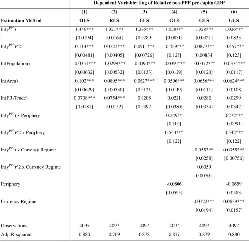
information on the area of each country was collected from the CIA World Factbook. We perform this estimation using three di¤erent estimation techniques, OLS, GLS and RLS, and pooling all observations in a unique cross-section.12 The estimation results are reported in Table 1. Columns
(1) to (3) show the results for the baseline speci…cation re‡ected in equation (2) for each of the three estimation techniques. As it can be seen from the …rst three columns of Table 1, the three techniques do not lead to substantially di¤erent coe¢cients for PPP-adjusted GDP per capita, its squared term and the other variables. Yet, the GLS estimation leads to greater standard errors which indicates the presence of heteroscedasticity or autocorrelation in the data. Moreover, the robust least squares estimation do not reveal any extreme outliers in the data. For these reasons, we are subsequently focusing on GLS estimates.
[Insert Table 1 (Short-Cut Estimation Results) here]
To make our regression speci…cation more ‡exible, in column (4) we allow the estimated relationship between PPP- and non-PPP-adjusted GDP per capita to di¤er for countries that are at di¤erent stages of economic development. To do so we include a "Periphery" dummy variable which equals 1 if a country’s level of PPP-adjusted GDP per capita in a given year is less than or equal to 50% of that of the United States and 0 otherwise. To capture the various ways in which the peripheral status of an economy could matter in this context, we allow the dummy variable to in‡uence both the intercept as well as the coe¢cients of PPP-adjusted GDP
10All three variables are expressed relative to the corresponding value for the U.S..
11Prados de la Escosura (2000) argues that international price level di¤erences observed during the period
1950-1990 provide a good approximation of the corresponding di¤erences in the 19th century and early 20th century. This may seem at …rst as a rather heroic assumption. Yet, both the results obtained by him as well as our results reported below, seem to attest to that assumption.
12The advantage of generalized over ordinary least squares is that it allows to account for potential
per capita. As the results of column (4) indicate, this e¤ect seems to be primarily operating through the slope coe¢cients.
In column (5) we introduce an additional dummy variable to account for the fact that the 1950-1990 period used for the estimation of equation (2) encompasses both the more stable -in terms of exchange rate volatility- Bretton Woods era as well as the more turbulent post-1970 era. This "Currency Regime" dummy, which we also interact with the income terms, allows to separate the two eras and capture di¤erences in the relationship between PPP- and non-PPP-adjusted GDP across the two regimes. As the results of column (5) indicate, the nature of the relationship seems to indeed vary with the exchange rate regime.
Finally, in column (6) we add both the "Periphery" and the "Currency Regime" dummies to allow for both variation across di¤erent levels of economic development and exchange rate regimes in our estimated relationship between PPP- and non-PPP-adjusted GDP. We also include all the corresponding interaction terms with lnyP P P and (lnyP P P)2 apart from the interaction of the
squared income term with the currency regime dummy, which was shown to be insigni…cant in column (5). This speci…cation generates the best possible …t for the data,13 while the resulting
estimation results appear to be very much in line with those of columns (3), (4) and (5).
2.2
Nominal GDP Estimates, 1870-1949
Having estimated the relationship between PPP-adjusted and non-PPP-adjusted GDP per capita relative to the United States for the period 1950-1990, we now use it to make out-of-sample predictions. Speci…cally, we employ this relationship in order to predict non-PPP-adjusted GDP for the period 1870-1949 for which we lack comprehensive data.
To make these predictions we use the estimated coe¢cients of column (6) combined with the PPP-adjusted GDP per capita data provided by Maddison (2001), expressed in current prices.14
This source is also used to obtain population …gures for this earlier time period and to extend our "Periphery" dummy variable accordingly. For the "Currency Regime" dummy we follow Prados de la Escosura (2000) and assign to the classical gold standard period (1870-1913) the same value as during the Bretton Woods era, as both regimes essentially imposed …xed exchange rates. The remaining years during the world wars and the interwar period are treated as equivalent in terms of the currency regime to the post-1970 period. Finally, in cases where there have been areal changes we adjust the area of each country accordingly.15
13We assess the speci…cation …t based on the adjusted R-squared coe¢cients, which in the case of GLS can
be calculated in multiple ways. Here it corresponds to the squared correlation coe¢cient between the predicted value ofynoni P P P and its observed value.
14Maddison’s GDP …gures are expressed in constant 1990 prices. These are converted in current price terms
to make them comparable to the Penn World Tables current price GDP series that was used for the estimation of equation (2). This conversion is done by multiplying the original …gures with a 1990-base year U.S. Consumer Price Index, taken from Measuring Worth (www.measuringworth.com/uscpi).
Following this approach, we can construct estimates for nominal GDP per capita in current prices relative to the United States and implied PPP-factors for a set of 68 countries spanning the period from 1870 to 1949.16 Out of these 68 countries, we are able to obtain complete 80-year
time series for 57 countries and long series with more than 30 years of observations covering the post-1900 period for additional 6 countries.17 The resulting sample is also quite representative
as it spans all …ve continents of the world and represents countries of di¤ering levels of economic development and political-economic systems.
To provide a sense of the quality of our estimates, in Figure 1 we compare our estimated values of relative non-PPP-adjusted GDP per capita for the case of Great Britain with the actual values obtained from available historical national accounts data. We chose the case of Britain as an example, since it is the country with the greatest availability of good quality historical statistics and the only one for which this comparison is possible in all years from 1870 to 1949.18 In
addition, Figure 1 also includes the corresponding level of per capita GDP of Britain relative to the United Stated in PPP-adjusted terms based on Maddison’s data in order to give an idea of how the PPP-adjusted and non-PPP-adjusted …gures di¤er in the period of interest.
[Insert Figure 1 (British Relative per Capita GDP) here]
As it can be seen from the …gure, our estimated nominal GDP series matches very closely the actual one, indicating that our approach based on the "short-cut" method does indeed generate reasonable estimates. Moreover, as the signi…cant gap between the relative PPP-adjusted GDP series from Maddison and the non-PPP-adjusted series indicates, this close match between our non-PPP-adjusted GDP estimates and the actual ones is not driven by the absence of relative price di¤erences between Britain and the U.S.. In fact, as it is clearly visible in the …gure, the British price level was substantially lower than that of the U.S. during all the years from 1870 to 1949, although this gap fell over time as British prices converged to American ones.
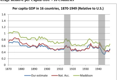
Apart from the case of Britain, this comparison of actual and estimated nominal GDP per capita can be performed for a few more countries for which historical nominal GDP time series are available. Based on information provided by Mitchell (2008) as well as by Smits, Woltjer, and Ma (2009), we were able to obtain such series for the period prior to 1949 for 16 countries -excluding the U.S..19 Figure 2 displays the weighted average of each of the three relative GDP
series for this set of 16 countries with weights based on each country’s aggregate PPP-adjusted
For all other countries the analysis is conducted based on their contemporary borders.
16The implied PPP-factor can be calculated by dividing the value of estimated non-PPP-adjusted GDP per
capita with the corresponding PPP-adjusted one.
17A detailed list of the countries and years of coverage can be found in the Appendix.
18As stated in the Appendix Britain and the United States are the only countries for which we have a complete
nominal GDP series as well as exchange rates going back to 1870.
19A list of these countries and the years of data coverage can be found in the appendix. Conversion to U.S.
level of GDP. Similar to the case of Britain, we can see that our estimated non-PPP-adjusted GDP series matches very closely the values obtained from existing historical national accounts statistics, while the PPP-adjusted series based on Maddison’s data di¤ers substantially.
[Insert Figure 2 (Average Relative per Capita GDP - 16 Countries) here]
This discrepancy is also evident if the root mean square errors (RMSE) for the deviation of our estimated nominal GDP values from the actual ones is calculated for these 16 countries. This can be then compared to the corresponding RMSE of the deviation of Maddison’s real GDP series from the actual nominal series. This error is 22% for our estimated series and 44% for Maddison’s series.20 Taking also into account the relative size of countries and calculating
weighted errors, the discrepancy is even more striking with the error being on average only 16% for our estimated series and 38% for the Maddison series.
3
World Trade Evolution, 1870-1949
Having constructed estimates for nominal GDP per capita for a large number of countries, we now turn to combine these estimates with the nominal export and import data assembled by Barbieri, Keshk, and Pollins (2009) to calculate trade shares going back to 1870.21 When doing
so, we follow the standard practice of summing up for each country the total value of exports and imports and dividing this value with our estimate of aggregate nominal GDP. This corresponds to the above estimated value of non-PPP-adjusted GDP per capita multiplied by the respective population …gures from Maddison (2001).
Based on the available trade data and our nominal GDP estimates, we are able to calculate trade shares for 51 countries, in addition to the U.S.. Among this set of countries, we have 24 countries for which we are able to track the complete evolution of trade shares for all non-war years -1870-1913 and 1920-1938- as well as a total of 43 countries for which our estimated trade shares series span more than 20 years. This greatly increases the available information on historical trade shares compared to the case were only non-estimated nominal GDP data from available historical sources are used. Based on the latter sources, we can construct trade shares for just 14 countries, out of which complete series covering all non-war years can only be calculated for six.22
To assess the quality of our estimated trade shares, in Figure 3 we display the evolution of Britain’s trade share over the period from 1870 to 1949, using three possible measures. The blue 20These errors are substantially lower during the First Globalization Era (20% for our estimate and 39% for
the Maddison series) than during the interwar period (26% and 57% respectively.)
21The data are available on-line through the Correlates of War project: http://correlatesofwar.org.
22The complete list of all countries and years for which trade shares can be constructed based on estimated
line corresponds to our estimated trade share, while the red line uses instead of our estimated non-PPP-adjusted GDP …gures the actual values taken from the available historical sources. In addition to those two measures, we also provide the trade share that would result if one would simply divide the sum of exports and imports by the total value of PPP-adjusted GDP reported by Maddison (2001) in‡ated with the U.S. Consumer Price Index. This is the practice followed by most of the existing literature and the series obtained this way is depicted by the green line. We add this third measure in order to see the extent to which combining PPP-adjusted GDP data with non-PPP-adjusted trade data would bias the implied trade shares.
[Insert Figure 3 (British Trade Share) here]
As Figure 3 demonstrates, the common practice of denominating nominal trade data with real GDP leads to a sizeable underestimation of the British trade share prior to 1950. The resulting discrepancy is substantial, particularly for earlier years, during which the price level of Britain was signi…cantly lower than that of the United States. In stark contrast to this, we see that our estimated trade share series matches closely the actual one, as it was the case with our nominal GDP estimates in Figure 1.
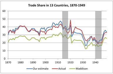
Moving beyond the case of Britain, Figure 4 presents the corresponding comparison in terms of trade shares for the 13 countries for which non-estimated nominal GDP data are available.23
The displayed series is a weighted average of the trade shares of all countries with weights based on each country’s fraction in the sum of the 13 countries’ GDP. As it was the case in Figure 3, our estimated series matches closely the actual one, while both exceed greatly the one based on the PPP-adjusted GDP series of Maddison.24 Moreover, a calculation of the corresponding root
mean square errors reveals that our estimated series on average deviates by only 23% from the actual series, while the series based on PPP-adjusted GDP deviates in average by 39% from the actual series.25 Weighting these deviations with each country’s share of aggregate GDP, leads to
a RMSE for our estimated series of only 17%, while the corresponding error of the series based on PPP-adjusted GDP is 35%.
[Insert Figure 4 (Average Trade Share - 13 Countries) here]
Having established the quality of our historical trade share estimates, we proceed now to discuss what they imply for the evolution of trade globally as well as across di¤erent regions of the world. This information is displayed in the following two …gures. First of all, Figure 5 23In this …gure we omit the Netherlands, which constitutes a clear outlier with an implied trade share in non-war
years during the period 1870-1939 averaging around 158% and occasionally reaching values of 300%.
24This is due to the fact that during the time period under investigation all countries of the world -with the
exception of Australia in some years- had, according to our estimates, lower price levels than the United States.
25As it was the case with our estimated nominal GDP values, these deviations are substantially smaller during
depicts how the share of international trade in terms of GDP evolved for the world as a whole. Here again, the blue line depicts our estimate that denominates the existing nominal trade data with our estimated nominal GDP series, while the green line corresponds to the one obtained if the real GDP data of Maddison (2001) are used instead. Both series are based on trade shares from the same 51 countries mentioned above weighted by each countries share in total GDP. In addition, Figure 5 also includes the equivalent world trade share series for the post-1950 period using information on the trade shares for the same set of 51 countries reported in the Penn World Tables and weighted correspondingly. We include this series in order to document how well our estimated pre-1950 global trade share series lines up with the conventional post-1950 wisdom regarding world trade.
[Insert Figure 5 (World Trade Share) here]
As Figure 5 documents, our estimated world trade share series, the blue line, is characterized by a secular rise during the …rst globalization era (1870-1913) and a sharp subsequent decline during the interwar period (1919-1939). Thus, qualitatively our series appears in line with the narrative o¤ered by Estevadeordal, Frantz, and Taylor (2003) as well as Jacks, Meissner, and Novy (2011) regarding the pre-World-War-II evolution of world trade.26 Yet, quantitatively our
estimated trade shares are much larger than the incorrectly calculated one, depicted by the green line, that one would obtain by dividing the nominal trade data with real GDP. Speci…cally, our estimates suggest that the share of world trade increased from 18% in 1870 to 32% during the …rst globalization era, while an incorrect calculation that does not fully account for purchasing power di¤erences across countries would reduce these numbers to 14% and 23% respectively. Similarly, during the interwar period, while according to our estimates the share of world trade fell from a pre-war level of 32% down to 11% in 1939, the incorrect trade share series displays a much smaller reduction from 23% to 10%. Regarding the magnitude of the discrepancy between the two series, this on average appears to be about 5.5 percentage points, which corresponds to an underestimation of the global trade share by 24%. It should be stressed, though, that this discrepancy is greater during the …rst globalization era than during the interwar period -6.5 versus 3.4 percentage points- due to the relative price convergence that took place over time.27
Moreover, the evolution of the world trade share implied by our estimates appears also to connect well with the post-1950 series based on Penn World Tables data. According to our 26Like many of the existing contributions in the literature, we take 1870 as the starting point of the …rst
globalization era. This is partial due to the lack of comprehensive trade statistics that go back even further in time. In principle, as O’Rourke and Williamson (2002) and Jacks (2005) have pointed out the …rst globalization era could potentially be extended by another 20 to 50 years by taking its starting point to be 1850 or even to 1820.
27It should be noted that the discrepancy between the two series would be even higher had the picture excluded
estimates, during the late 1940s world trade ‡uctuated in a band between 17.5% and 20.5% of GDP, which is very similar to the movements observed in the 1950s and 1960s during which the world trade share ‡uctuated between 18.5 and 21.5%. Thus, both our estimated series and the PWT series indicate that international trade was very stable during the …rst 25 years after World War II, averaging at a level of 19.5% of GDP and with a standard deviation of just 1 percentage point. Moreover, our historical trade series reveals that the level of trade openness that the world reached in 1913 at the peak of the …rst globalization era was not reached again globally before 1974. This con…rms the evidence regarding the rebound of international trade based on manufacturing products and merchandise trade presented by Beenstock and Warburton (1983), Krugman (1995) and O’Rourke and Williamson (1999).
In contrast, the incorrectly calculated series suggests that the value of world trade in the late 1940s was around 14% of world GDP, which seems unreasonably low in light of the trade activity observed during the 1950s and 1960s. Similarly, this series suggests that the share of world trade at its pre-World-War-I peak was equivalent to that observed during the earlier 1950s, which contradicts the aforementioned evidence. These observations suggest that an incorrect calculation of trade shares, which does not take into account relative price di¤erences across countries, may lead to a distorted picture regarding the evolution of world trade prior to 1950 and a profound underestimation of the rise and fall that took place from the …rst globalization era to the end of World War II.
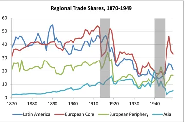
Looking beyond the global picture, in Figure 6 the evolution of world trade over the period 1870-1949 is broken down into separate series for four key regions of the globe: the European core, the European periphery, Latin America and Asia.28 A comparison of the regional series
reveals that the rise and fall of world trade that occurred from 1870 to 1939 was not uniformly experienced across all regions of the world. While in terms of levels, trade shares at the start of the …rst globalization era were highest in Latin America and lowest in Asia, over this 40-year period, though, the European core economies overtook the Latin American ones, in which the share of international trade remained fairly constant. This upward trend was also experienced by the economies of the European periphery and of Asia, but to a lesser extent.
[Insert Figure 6 (Regional Trade Shares) here]
Following the …rst World War and the subsequent Great Depression it was again the European core economies that witnessed the greatest implosion of trade. Yet, during this period the experience of Latin American and European peripheral economies was not di¤erent, as trade shares dropped to levels that were even lower than those prevailing during the …rst globalization era. Interestingly, though, this downward trend was not shared by the Asian economies, which
-according to our estimates- did not witness a disruption of the pre-World-War-I trade expansion during the interwar period but rather a continuation of pre-existing trends.
In Figure 6 we have avoided adding the corresponding incorrectly calculated trade shares that were shown in Figure 5 in order to not overcrowd the diagram. Yet, we should mention here that the same remarks as those made above apply also for all the regional trade shares series. Thus, trade shares based on a PPP-adjusted income measure are consistently lower than the "true" ones based on non-PPP-adjusted GDP. Moreover, the degree of underestimation is highest for the poorest regions of the world, which had the lowest relative price levels compared to the United States.
4
Determinants of Bilateral Trade Flows, 1870-1939
In addition to our discussion of the evolution of national, regional and global shares of interna-tional trade from 1870 to 1949, in the present paper we also seek to investigate more carefully what determined these trade ‡ows across countries over this period. We embark on this inves-tigation in order to assess the extent to which an analysis of trade ‡ows based on real income values and nominal trade data, which is the approach followed by most of the existing literature, would lead to incorrect inferences regarding the determinants of trade during this important historical period.
4.1
Gravity Regression Results
To analyze trade ‡ows across countries we pursue a gravity approach, which by now has become standard in the empirical literature on international trade. According to this approach, the level of trade between two economies is assumed to be driven by the size of as well as the degree of inward and outward resistance exhibited by each economy.29 The former is typically
captured by each economy’s aggregate level of GDP, while the latter re‡ects various types of barriers to international trade. In the historical context of the …rst globalization era and the interwar period the two main factors in‡uencing the strength of these barriers were the extent of tari¤ protection and the participation in the gold standard. In this respect we follow the work of Estevadeordal, Frantz, and Taylor (2003), Jacks, Meissner, and Novy (2011) and others who have analyzed bilateral trade ‡ows during these periods based on a gravity framework. Speci…cally, we estimate the following regression speci…cation:
ln(T radeijt) = + Y ln(YitYjt) + T ln(1 +
tit+tjt
2 ) + GGoldijt+ ij + t+"ijt: (3)
T radeijt refers to the sum of trade ‡ows between two countries i and j at time t; Yit and Yjt
denote aggregate GDP in the two countries, tit and tjt correspond to the average tari¤ rate
in the two countries,30 while Gold
ijt is a dummy variable equaling one if both countries i and
j were on the gold standard at time t: The term ij denotes a pair …xed e¤ect capturing any
time-invariant pair-speci…c factors, such as the distance between two countries, the existence of a common border or the presence of a common language, that could in‡uence the extent of trade between countriesiandj:31 Finally, t denotes a time …xed e¤ect capturing general time-varying
trends, such as the change in world income or the available technology.32
Both our trade ‡ows and aggregate GDP variables are expressed in current prices, with the former being taken from Barbieri, Keshk, and Pollins (2009) and the latter being estimated as discussed in Section 2. The average tari¤ data are from Clemens and Williamson (2004) and updated with the information provided by Schularick and Solomou (2011),33 while the coding of
the gold standard variable is based on the information provided by O¢cer (2008).34 We focus
our analysis on the role of income, tari¤s and the gold standard in determining trade between countries during the period from 1870 to 1939, as these are the variables that have attracted most of the attention in the literature. An important di¤erence, though, between our approach and that of the existing literature is that we estimate the above speci…cation using non-PPP-adjusted income and trade data. Thus, do not combine PPP-adjusted income data with non-PPP-adjusted trade ‡ows, which -as we show below- would tend to bias the estimated coe¢cients.35
We estimate equation (3) separately for the …rst globalization era (1870-1913) and the interwar period (1919-1938) using an unbalanced panel of countries. In the former period this includes 202 30Given that available tari¤ data for the period of interest only provide information on average tari¤ rates per
country, we use the mean of the prevailing average tari¤ rates in the two countries to proxy for the actual bilateral tari¤ rate which is not observed.
31We also considered an alternative speci…cation with country …xed e¤ects instead of pair …xed e¤ects. Such a
speci…cation has the advantage of allowing us to explicitly control for the e¤ect of key time-invariant pair-speci…c characteristics such as distance, shared border or common language. Given, though, that the results of this alternative speci…cation are not substantially di¤erent and given the more parsimonious nature of a speci…cation with pair …xed e¤ects, we chose not to present any results based on this alternative speci…cation, which may be subject to biases due to unobserved heterogeneity across pairs.
32Our speci…cation does not explicitly account for transportation costs due to a lack of data at the country or pair
level. Yet, the inclusion of pair …xed e¤ects, which among others account for the distance between two countries, and the inclusion of time …xed e¤ects, which among others re‡ect the state of technology, implicitly allows us to do so. This is because, as discussed in Estevadeordal, Frantz, and Taylor (2003), distance and technology were the two main factors driving the evolution of transportation costs. Alternatively, we also considered a speci…cation which includes distance-decade interaction terms to explicitly account for the changing importance of distance-related transportation costs. This, however, did not lead to qualitatively di¤erent results compared to speci…cation (3) and for this reason we do not present more details.
33We would like to explicitly thank Michael Clemens, Moritz Schularick, Solomos Solomou, and Je¤rey
Williamson for being kind enough to share their data with us.
34This information is available on-line at eh.net/encyclopedia/article/o¢cer.gold.standard and we would also
like to thank Lawrence O¢cer for kindly providing us with the data tables included in the article.
35As we explain below, though, we do compare our results with those obtained when PPP-adjusted income
distinct country pairs and in the latter 296.36 The results of this estimation based on OLS are
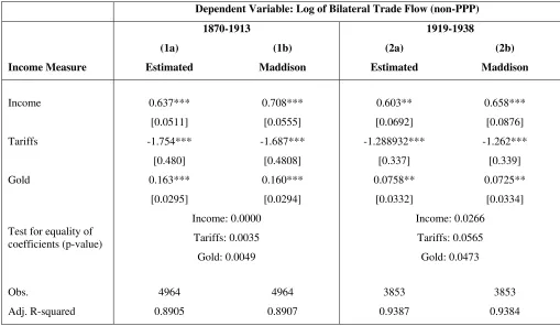
reported in Table 2. The left panel of the table displays the results for the 1870-1913 period, and the right one for the 1919-1938 period. In each panel we compare the estimated coe¢cients with those obtained if the PPP-adjusted GDP data of Maddison (2001) in‡ated with the U.S. CPI are used instead of our estimated non-PPP-adjusted GDP values. The regressions displayed in each of the two panels are estimated as two seemingly unrelated equations, using robust estimators of the simultaneous variance-covariance matrix. At the bottom of each panel, we report for each of the two periods the corresponding p-values for the tests of the equality of the coe¢cients on income, tari¤s and the gold standard.
[Insert Table 2 (Gravity Regressions - Full Sample) here]
Overall the results displayed in Table 2 con…rm the importance of income levels, tari¤s rates and gold standard membership as important determinants of bilateral trade ‡ows. In both periods the coe¢cients of all three variables are statistically signi…cant and have the expected signs. Higher income levels in either country led to increased bilateral trade, while greater tari¤ protection had the opposite e¤ect. Moreover, bilateral trade between countries was promoted through adherence to the gold standard.37 We should note, however, that the low p-values of
the tests of equality for the coe¢cients on each regressor at the bottom of each panel imply that the estimated coe¢cients on all three variables statistically di¤er depending on the type of GDP measure used in the estimation. Speci…cally, we see that the e¤ect of income tends to be overestimated, while the e¤ect of tari¤s and the gold standard tend to be underestimated if a PPP-adjusted income measure is used instead of a non-PPP-adjusted one. The intuition for this bias is simple and stems from the fact that the relative dispersion of PPP-adjusted income is much lower than that of non-PPP-adjusted income, as the latter encompasses not only the dispersion in living standards but also that in price levels.
An important caveat to the above interpretation of the estimation results in Table 2 is that they may be subject to endogeneity biases. A likely source of such bias is the gold standard dummy, as Estevadeordal, Frantz, and Taylor (2003) and Meissner (2005) have argued that pre-existing trade linkages between countries in‡uenced the adoption of the gold standard. Thus, to ensure that our results are not driven by this type of endogeneity we follow Estevadeordal, Frantz, and Taylor (2003) and instrument the Gold dummy variable with the product of the
logarithm of each partner country’s average distance from all countries participating in the gold standard in any given period. The results of this instrumental-variable estimation are displayed 36The unbalanced nature of the panel has little e¤ects on the estimation results. Even when we re-estimate
our speci…cation in a balanced panel which includes 50 pairs during the pre-1913 period and 97 pairs during the interwar period the results are qualitatively unchanged.
37In this respect our …ndings con…rm those of Estevadeordal, Frantz, and Taylor (2003), Lopez-Cordova and
in Table 3 for both sub-periods.38 In either case the instrumentation strategy does not lead to
qualitatively di¤erent results, although the point estimates of the income coe¢cients are lower than the corresponding OLS estimates while those for tari¤s and the gold standard higher.39
Moreover, as in Table 2, when a PPP-adjusted GDP measure is used instead of a non-PPP-adjusted one we still observe an overestimation of the e¤ect of income and an underestimation of those of tari¤s and the gold standard.
[Insert Table 3 (Gravity Regressions - IV Results) here]
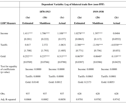
An additional concern regarding our …ndings above of a relative underestimation of the e¤ects of tari¤s and the gold standard and an overestimation of the e¤ect of income is that this may be due to the fact that our nominal GDP data are estimated. To test that this is not the case, we re-estimate our main speci…cation (3) using only the country-pairs for which actual nominal GDP data are available from historical sources. The results from these regressions are reported in the two panels of Table 4. In each panel the …rst column reports the estimated coe¢cients obtained with our estimated nominal GDP data, the second column those based on the real income data of Maddison (2001) and the third column those when non-estimated nominal GDP data are used.40 To ease comparisons between the results of each column we have kept the sample
constant across all three speci…cations, using the information from just 26 country-pairs in the …rst subperiod and 55 pairs in the second.
[Insert Table 4 (Gravity Regressions - Restricted Sample) here]
This restriction to a substantially smaller sample obviously implies greater standard errors and lower statistical signi…cance. Yet, the results of Table 4 appear to be generally in line with the …ndings from Tables 2 and 3. Income levels have a strong positive e¤ect on bilateral trade ‡ows, which e¤ect, however, tends to be overestimated when real GDP values are used instead of nominal ones. The participation in the gold standard has a signi…cantly positive e¤ect on trade ‡ows and its magnitude tends to be underestimated when real GDP values are employed. Finally, tari¤s have a statistically signi…cant negative e¤ect at least during the interwar period, which again tends to be underestimated in the gravity regressions based real GDP data.41 Furthermore,
even in this restricted sample, a comparison of the regression coe¢cients between columns (1) and (2) as well as (2) and (3) in both panels reveals that they are statistically di¤erent from 38As following World War I all countries except for El Salvador had abandoned the use of gold until 1921, we
are forced in the second subperiod to restrict our estimation to the years from 1921 to 1938.
39To faciliate the comparison with the OLS estimates, the last part of the panel shows the correponding OLS
results for this reduced sample.
40The sources for these data are discussed in Section 2.
41We suspect that the insigni…cance of the average tari¤ variable during the …rst globalization era is driven
one another, as the low p-values in the bottom of the table indicate. This con…rms that the overestimation of the income e¤ect and the underestimation of the tari¤ and gold-standard e¤ects in gravity regressions where nominal trade data are combined with real instead of nominal GDP is not an artifact of the estimated nature of our nominal GDP data.
4.2
Relative Contributions of Income Growth, Tari¤s and the Gold
Standard in the Rise and Fall of Trade
Having established the importance of income growth, tari¤ rates and the expansion of the gold standard in determining bilateral trade ‡ows during the period from 1870 to 1939, we now turn to an assessment of the relative importance of these three factors in comparison to common global trends. We perform this assessment separately for each subperiod based on the coe¢cients estimated in column 1 of panels 1 and 2 in Table 2. Thus, we use the estimation results based on non-PPP-adjusted income values to avoid the potential biases discussed above.
In order to assess the relative importance of income growth, tari¤ rate changes, participation in the gold standard as well as common global trends for trade we perform a counterfactual analysis in the spirit of Baier and Bergstrand (2001) and Estevadeordal, Frantz, and Taylor (2003). We calculate the counterfactual trade levels that would have resulted between any two pair of countries i and j if only one of the four factors had changed over time and the other
variables had remained constant. Speci…cally, suppose that the variable of interestxhad changed
by the amount xt 1 between periods t and t 1: Then, if x is the coe¢cient of variable x
derived from the gravity model, the counterfactual level of trade in period t would be:
TradeC
ijt= exp[ x xt 1] Tradeijt:
To assess the role of common global trends, which among other things capture the extent and importance of changes in the transportation technology, we rely on the estimated year …xed e¤ects from each speci…cation. This is because the …xed e¤ects capture how di¤erent trade ‡ows are ceteris paribus in a given year compared to the initial year. Thus, with tbeing the estimate
of the time …xed e¤ect in period t; the corresponding counterfactual level of trade in period t
would be
TradeC
ijt = exp[ t] Tradeijt:
since we are interested in the contribution of global trends over the whole course of each of these two periods, we use the values of the …xed e¤ects in the …nal years of each period - i.e. the values in 1913 and 1938 - in our calculations.
On average, during the …rst globalization era the product of nominal incomes grew by 3.8% per year, implying that the typical country experienced an annual GDP growth rate of 1.9% during this period. During the interwar period, the corresponding growth rate was 3.3%. As for our average tari¤ measure, on average the per-pair tari¤ rate fell by 0.05 percentage points per year during the …rst globalization era and rose by 0.03 percentage points during the interwar period. Finally, our gold standard dummy - which essentially re‡ects the fraction of pairs being on gold at a given time - on average increased by 1.5 percentage points per year during the …rst globalization era and fell by 0.55 percentage points during the interwar period.
Looking at these two periods as a whole the following trends should be noted. During the …rst globalization era the level of non-PPP-adjusted GDP per country grew on average by approximately 80%, tari¤s fell by 2.3 percentage points and the participation in the gold standard increased by 65 percentage points.42 During the interwar period the corresponding income growth
rate was on average 33.5%. At the same time, average tari¤s increased by 11 percentage points and adherence to the gold standard declined by 0.6 percentage points.43 Finally, the value of the
…xed e¤ects indicating the globally experienced changes in the log-level of bilateral trade over the two periods of interest is 0.67 in 1913 and -0.82 and 1939.
[Insert Table 5 (Counterfactual Analysis) here]
Table 5 above reports the results of this counterfactual analysis. Given the income coe¢cients reported in Table 2, the cumulative growth performance of the world economy implies that income growth contributed approximately 64% to trade growth during the …rst globalization era and about 33% during the interwar period. To be more precise, the value of 64.2% for income during the pre-1913 period implies that trade would have been 64.2% lower than it actually was in 1913 had income not increased between 1870 and 1913. Similarly for tari¤s, we have that their fall contributed approximately 4% to trade growth during the …rst globalization era and their rise during the interwar period alone led to a 16% fall in world trade. Regarding the contribution of the gold standard our gravity regression results imply that its expansion during the …rst globalization era contributed to a 10% increase in world trade, while its disintegration during the interwar period played only a minor role for the evolution of bilateral trade relative to that of income growth and tari¤ spikes. Finally, the values of the …xed e¤ects imply that 42This means that if hypothetically in 1870 there were no pair of countries trading with one another whose
currencies where both …xed to gold, by 1913 65% of all sample pairs were jointly on the gold standard.
43This low observed change in the gold standard variable is due to the fact that no expansion of the gold
common global trends contributed 49% to trade growth during the …rst globalization era, and would have led to a 128% decline in trade during the interwar period had not other factors, such as income growth, counterbalanced this e¤ect.
Viewed from the perspective of the literature our …ndings for the …rst globalization era are line with those of Estevadeordal, Frantz, and Taylor (2003) and Jacks, Meissner, and Novy (2010) who attribute approximately 60% of pre-World-War-I trade expansion to income growth. They also con…rm the relative unimportance of tari¤ movements during that period in comparison to global trends such as the decline in transportation costs. Moreover, similar to Lopez-Cordova and Meissner (2003) we also …nd a relatively small contribution of the gold standard expansion of approximately 10%. Regarding the interwar period, our estimated contributions of income growth and tari¤ movements are close to those of Estevadeordal, Frantz, and Taylor (2003), who …nd the former to be approximately 34% and the latter 22%. Yet, we …nd the disintegration of the gold standard that took place over this period to be substantially less important than existing studies and attribute the sharp fall of world trade that took place over the interwar period mostly to adverse global trends.44
5
Concluding Remarks
The recent debate regarding the causes and the consequences of the increased economic integra-tion that countries and regions of the world are experiencing today has triggered an increased interest in the globalization trends that existed prior to World War II. This interest stems from the conviction of a growing number of economists and economic historians that shedding light on the various factors that drove the expansion of world trade during the …rst globalization era (1870-1913) and its backlash during the interwar period (1919-1939) can enhance our under-standing of contemporary developments.
A major di¢culty in the context of this literature, though, has been the relative scarcity national account data compared to the post-War-World-II period. As a consequence, in order to calculate trade shares prior to 1950 most researchers have combine PPP-adjusted GDP measures, such as those of Maddison (2001), with nominal trade data, an approach which is subject to systematic biases.
Contrary to existing work, this paper provides estimates of trade shares based on non-PPP-adjusted GDP values which we estimate via the short-cut method. Our estimates indicate that trade shares during the 1870-1949 period were on average 32% higher compared to existing 44Our …nding of the relative unimportance of the evolution of the gold standard during the interwar period for
accounts and the world’s level of openness to trade in 1913 had been comparable to that in 1974. This implies that the rise and fall of world trade that took place over this period was much more pronounced than previously documented.
Furthermore, employing our nominal GDP estimates in standard gravity regressions, we re-assess the determinants of bilateral trade ‡ows during this time period and the relative impor-tance of income growth, tari¤ movements and the evolution of the gold standard. Our approach di¤ers from existing work that has performed such estimations using PPP-adjusted income even though the available trade data are expressed in nominal terms. In this context we …nd that the existing literature has tended to overemphasize the role of income movements relative to tari¤s changes and the evolution of the gold standard.
As a …nal note, we would like to stress that although in this paper we have focused on analyzing the evolution of world trade between 1870 and 1949 and its determinants, we believe that our contribution extends beyond that. The estimates of non-PPP-adjusted GDP and trade shares that we provide via the "short-cut" method for a large set of countries can provide useful benchmarks for any subsequent research on the matter. Moreover, in the absence of alternative more comprehensive historical sources, we believe that our estimates of nominal income and trade shares can be of great value-added to many researchers interested in this historical period.
References
Anderson, J. E., and E. van Wincoop (2003): “Gravity with Gravitas: A Solution to the Border Puzzle,” The American Economic Review, 93(1), 170–192.
Baier, S. L.,and J. H. Bergstrand(2001): “The Growth of World Trade: Tari¤s, Transport Costs, and Income Similarity,” Journal of International Economics, 53(1), 1–27.
Balassa, B. (1964): “The Purchasing Power Parity Doctrine: A Reappraisal,” Journal of Political Economy, 72(6), 584–596.
Barbieri, K., and O. Keshk (2012): “Correlates of War Project Trade Data Set Codebook, Version 3.0,” Online: http://correlatesofwar.org.
Barbieri, K., O. Keshk, and B. Pollins (2009): “TRADING DATA: Evaluating our As-sumptions and Coding Rules,” Con‡ict Management and Peace Science, 26(5), 471–491.
Beenstock, M., and P. Warburton (1983): “Long-Term Trends in Economic Openness in the United Kingdom and the United States,” Oxford Economic Papers, 35(1), 130–135.
Clemens, M. A., and J. G. Williamson (2004): “Why Did the Tari¤-Growth Correlation Change after 1950?,” Journal of Economic Growth, 9(1), 5–46.
Eichengreen, B., and D. A. Irwin (1995): “Trade Blocs, Currency Blocs and the Reorien-tation of World Trade in the 1930s,” Journal of International Economics, 38(1-2), 1–24.
Estevadeordal, A., B. Frantz, and A. M. Taylor (2003): “The Rise and Fall of World Trade, 1870-1939,” The Quarterly Journal of Economics, 118(2), 359–407.
Frankel, J. A., and D. Romer (1999): “Does Trade Cause Growth?,” The American Eco-nomic Review, 89(3), 379–399.
Heston, A., R. Summers, and B. Aten (2011): “Penn World Table Version 7.0,” Center for International Comparisons of Production, Income and Prices at the University of Pennsylvania.
Irwin, D. A., and M. Terviö (2002): “Does Trade Raise Income?: Evidence from the Twen-tieth Century,” Journal of International Economics, 58(1), 1–18.
Jacks, D. S. (2005): “Intra- and International Commodity Market Integration in the Atlantic Economy, 1800-1913,” Explorations in Economic History, 42(3), 381–413.
Jacks, D. S., C. M. Meissner, and D. Novy (2010): “Trade Costs in the First Wave of Globalization,” Explorations in Economic History, 47(2), 127–141.
(2011): “Trade Booms, Trade Busts, and Trade Costs,” Journal of International Eco-nomics, 83(2), 185–201.
Jacks, D. S., and K. Pendakur (2010): “Global Trade and the Maritime Transport Revolu-tion,” The Review of Economics and Statistics, 92(4), 745–755.
Kravis, I. B. (1984): “Comparative Studies of National Incomes and Prices,” Journal of Eco-nomic Literature, 22(1), 1–39.
Kravis, I. B., A. W. Heston, and R. Summers (1978): “Real GDP Per Capita for More Than One Hundred Countries,” The Economic Journal, 88(350), 215–242.
Krugman, P. (1995): “Growing World Trade: Causes and Consequences,” Brookings Papers on Economic Activity, 1, 327–377.
Lopez-Cordova, J. E., and C. M. Meissner (2003): “Exchange-Rate Regimes and Inter-national Trade: Evidence from the Classical Gold Standard Era,” The American Economic Review, 93(1), 344–353.
Maddison, A.(2001): The World Economy: Volume 1 - A Millennial Perspective. Development
Studies Center, OECD, Paris.
Meissner, C. M. (2005): “A New World Order: Explaining the International Di¤usion of the Gold Standard, 1870-1913,” Journal of International Economics, 66(2), 385–406.
Mitchell, B. R.(2008): International Historical Statistics: 3 Volume Set, 1750-2005. Palgrave
Macmillan, New York.
Officer, L. H.(2008): “Gold Standard,” EH.Net Encyclopedia, edited by Robert Whaples.
Officer, L. H., and S. H. Williamson (2012): “The Annual Consumer Price Index for the United States, 1774-2011,” MeasuringWorth.
O’Rourke, K. H., and J. G. Williamson (1999): Globalization and History: The Evolution of a Nineteenth Century Atlantic Economy. The MIT Press, Cambridge, MA.
(2002): “When Did Globalisation Begin?,”European Review of Economic History, 6(1),
23–50.
Prados de la Escosura, L.(2000): “International Comparisons of Real Product, 1820-1990: An Alternative Data Set,” Explorations in Economic History, 37(1), 1–41.
Samuelson, P. A. (1964): “Theoretical Notes on Trade Problems,” The Review of Economics and Statistics, 46(2), 145–154.
Schularick, M., and S. Solomou (2011): “Tari¤s and Economic Growth in the First Era of Globalization,” Journal of Economic Growth, 16(1), 33–70.
22
Table 1: Short-Cut Estimation Results
Dependent Variable: Log of Relative non-PPP per capita GDP
(1) (2) (3) (4) (5) (6)
Estimation Method OLS RLS GLS GLS GLS GLS
ln(yPPP) 1.446*** 1.321*** 1.356*** 1.058*** 1.328*** 1.026*** [0.0194] [0.0164] [0.0289] [0.0831] [0.0321] [0.0833] ln(yPPP)^2 0.114*** 0.0721*** 0.0911*** -0.459*** 0.0877*** -0.457***
[0.00481] [0.00405] [0.00726] [0.123] [0.00834] [0.123]
ln(Population) -0.0351*** -0.0299*** -0.0390*** -0.0391*** -0.0372*** -0.0374*** [0.00632] [0.00532] [0.0133] [0.0129] [0.0120] [0.0117] ln(Area) 0.102*** 0.0895*** 0.0627*** 0.0596*** 0.0656*** 0.0624***
[0.00629] [0.00530] [0.0121] [0.0119] [0.0111] [0.0108] ln(FR-Trade) 0.0708*** 0.0754*** 0.0208 0.0221 0.0282 0.0299
[0.0181] [0.0152] [0.0392] [0.0380] [0.0354] [0.0342]
ln(yPPP) x Periphery 0.249** 0.272***
[0.100] [0.0991]
ln(yPPP)^2 x Periphery 0.544*** 0.542***
[0.122] [0.122] ln(yPPP) x Currency Regime 0.0553** 0.0355***
[0.0258] [0.00756]
ln(yPPP)^2 x Currency Regime 0.0059
[0.00701]
Periphery -0.0806 -0.0659
[0.0595] [0.0583]
Currency Regime 0.0722*** 0.0639***
[0.0194] [0.0157]
Observations 4097 4097 4097 4097 4097 4097
Adj. R-squared 0.880 0.769 0.878 0.879 0.879 0.880
Notes: All variables except from dummies are relative to those of the United States; standard errors in brackets.
23
Figure 1: British Relative per Capita GDP
Figure 2: Average Relative per Capita GDP - 16 Countries
0 0.2 0.4 0.6 0.8 1 1.2 1.4 1.6
1870 1880 1890 1900 1910 1920 1930 1940
Per capita GDP of Britain, 1870‐1949 (Relative to U.S.)
Our estimate Nat. Acc. Maddison
0 0.2 0.4 0.6 0.8 1 1.2 1.4 1.6
1870 1880 1890 1900 1910 1920 1930 1940
Per capita GDP in 16 countries, 1870‐1949 (Relative to U.S.)
[image:24.612.119.496.406.664.2]24
Figure 3: British Trade Share
Figure 4: Average Trade Share - 13 Countries
0 10 20 30 40 50 60 70
1870 1880 1890 1900 1910 1920 1930 1940
British Trade Share, 1870‐1949
Our estimate Actual Maddison
0 10 20 30 40 50 60
1870 1880 1890 1900 1910 1920 1930 1940
Trade Share in 13 Countries, 1870‐1949
[image:25.612.113.498.445.697.2]25
Figure 5: World Trade Share
Figure 6: Regional Trade Shares
0 5 10 15 20 25 30 35 40 45 50
1870 1880 1890 1900 1910 1920 1930 1940 1950 1960 1970 1980 1990 2000
World Trade Share, 1870‐2000
Our Measure PWT Wrong Measures
0 10 20 30 40 50 60
1870 1880 1890 1900 1910 1920 1930 1940
Regional Trade Shares, 1870‐1949
[image:26.612.119.499.461.711.2]26
Table 2: Gravity Regressions – Full Sample
Dependent Variable: Log of Bilateral Trade Flow (non-PPP)
1870-1913 1919-1938
(1a) (1b) (2a) (2b)
Income Measure Estimated Maddison Estimated Maddison
Income 0.637*** 0.708*** 0.603** 0.658***
[0.0511] [0.0555] [0.0692] [0.0876] Tariffs -1.754*** -1.687*** -1.288932*** -1.262***
[0.480] [0.4808] [0.337] [0.339]
Gold 0.163*** 0.160*** 0.0758** 0.0725**
[0.0295] [0.0294] [0.0332] [0.0334]
Test for equality of coefficients (p-value)
Income: 0.0000 Income: 0.0266 Tariffs: 0.0035 Tariffs: 0.0565 Gold: 0.0049 Gold: 0.0473
Obs. 4964 4964 3853 3853
Adj. R-squared 0.8905 0.8907 0.9387 0.9384
27
Table 3: Gravity Regressions – IV Results
Dependent Variable: Log of bilateral nominal (non-PPP) trade flow
Estimation
Method 2SLS 2SLS OLS
1870-1913 1921-1938 1921-1938
(1a) (1b) (2a) (2b) (2a) (2b)
Income
Measure Estimated Maddison Estimated Maddison Estimated Maddison
Income 0.294** 0.363** 0.828*** 1.132*** 0.678*** 0.756***
[0.153] [0.172] [0.138] [0.233] [0.0733] [0.0926]
Tariffs -5.797*** -5.431*** -1.209*** -1.147*** -1.288*** -1.255***
[1.740] [1.806] [0.367] [0.393] [0.356] [0.358]
Gold 1.452*** 1.349** -0.654 -1.0938a 0.0749** 0.0701**
[0.517] [0.539] [0.625] [0.692] [0.0349] [0.0350]
1st Stage F-Stat. 18.825 16.204 26.789 23.849 - -
Adj. R-squared - - - - 0.9392 0.9389
Obs. 4964 4964 3726 3726 3726 3726
2SLS estimation results with pair and year fixed effects, not reported; “Gold” instrumented by the sum of the natural logarithms of the average distance of each country from all other countries on the gold standard; the reported first-stage F-statistic is the partial F-F-statistic testing the significance of the excluded instrument in the corresponding first-stage regression; included; robust standard errors in brackets.
28
Table 4: Gravity Regressions – Restricted Sample
Dependent Variable: Log of bilateral trade flow (non-PPP)
1870-1913 1919-1938
(1a) (1b) (1c) (2a) (2b) (2c)
GDP Measure Estimated Maddison Actual Estimated Maddison Actual
Income 1.411*** 1.706*** 1.108*** 1.0278*** 1.397*** 0.0484
[0.201] [0.222] [0.157] [0.0863] [0.117] [0.0552]
Tariffs 0.817 2.372 -1.0631 -2.380*** -2.194*** -4.0330***
[1.708] [1.793] [1.405] [0.771] [0.756] [0.853]
Gold 0.252*** 0.237*** 0.313*** 0.0679* 0.0640* 0.119***
[0.0769] [0.0766] [0.0788] [0.0387] [0.0386] [0.0425] Test for equality
of coefficients (p-value)
Income: 0.0000 Income: 0.0000 Income: 0.0000 Income: 0.0000
Tariffs: 0.0000 Tariffs: 0.0000 Tariffs: 0.0063 Tariffs: 0.0001
Gold: 0.0140 Gold: 0.0012 Gold: 0.2173 Gold: 0.0053
Obs. 937 937 937 628 628 628
Adj. R-squared 0.8868 0.8882 0.8858 0.9781 0.9782 0.9742
Notes: OLS estimation results with pair and year fixed effects, not reported; robust standard errors in brackets. *** significant at the 1% level; ** significant at the 5% level; * significant at the 10% level.
Table 5: Counterfactual Analysis
Total change in Trade explained by Gravity Model
Contributions of 1870-1913 1919-1938
Income 64.2% 33.1%
Tariffs 3.9% -15.5%
Gold Standard 10.0% -0.045%
[image:29.612.55.569.597.707.2]29
Appendix: List of Countries
Country Est. Nominal GDP
Act. Nominal GDP
Est. Trade Share Act. Trade Share
Region
Algeria 1870-1949
Argentina 1870-1949 1870-1949 Latin America
Australia 1870-1949 1870-1931 1920-1949 1920-1931
Austria 1870-1949 1870-1913,
1919-1938
European Core
Belgium 1870-1949 1870-1913, 1920-1939, 1946-1949 1870-1914, 1919-1940 1945-1949 1870-1913, 1920-1939, 1946-1949 European Core Bolivia 1945-1949
Brazil 1870-1949 1870-1949 Latin America
Bulgaria 1870-1949 1908-1917,
1919-1949
European Periphery
Canada 1870-1949 1926-1949 1920-1949 1926-1949
Chile 1870-1949 1870-1949 Latin America
China 1870-1949 1870-1940,
1942-1943, 1946-1949
Asia
Colombia 1900-1949 1900-1949 Latin America
Costa Rica 1920-1949 1920-1949 Latin America Czechoslovakia 1870-1949 1919-1939,
1945-1949
European Periphery
Denmark 1870-1949 1870-1940 1870-1940, 1945-1949
1870-1940 European Core
Ecuador 1939-1949 1939-1949 Latin America
Egypt 1870-1949 1937-1949
El Salvador 1920-1949 1920-1949 Latin America Finland 1870-1949 1920-1945 1919-1949 1920-1945 European Core France 1870-1949 1870-1913,
1920-1938 1870-1917, 1920-1949 1870-1913, 1920-1938 European Core
Germany 1870-1949 1870-1913, 1920-1944
European Core
Ghana 1870-1949
Greece 1870-1949 1870-1913,
1919-1940, 1945-1949
European Periphery
Guatemala 1920-1949 1920-1949 Latin America
Haiti 1945-1949
Honduras 1920-1949 1925-1949 1920-1949 1925-1949 Latin America Hong Kong 1870-1949
Hungary 1870-1949 1870-1913,
1919-1949
European Periphery
India 1870-1949
Indonesia 1870-1949
Iran 1870-1949 1870-1949 Asia
Iraq 1870-1949 1932-1949 Asia
Ireland 1870-1949 1922-1949 European Core
Italy 1870-1949 1870-1942,
1946-1949
European Periphery
Jamaica 1870-1949
Japan 1870-1949 1885-1940 1870-1944 1885-1940 Asia
30
List of Countries (cont.)
Country Est. Nominal GDP
Act. Nominal GDP
Est. Trade Share Act. Trade Share
Region
Korea 1870-1949 1911-1940 1888-1905 Asia Malaysia 1870-1949
Mexico 1870-1949 1925-1949 1870-1913, 1918-1949
1925-1949 Latin America
Morocco 1870-1949 1870-1911 Myanmar 1870-1949
Nepal 1870-1949 1920-1923 Asia
Netherlands 1870-1949 1870-1913, 1921-1939 1870-1913, 1915-1949 1870-1913, 1921-1939 European Core
New Zealand 1870-1949 1920-1949
Nicaragua 1920-1949 1920-1949 Latin America
Norway 1870-1949 1905-1913,
1919-1940 1945-1949
European Core
Panama 1945-1949
Paraguay 1870-1949 1939, 1946-1949 Latin America
Philippines 1870-1949
Poland 1870-1949 1920-1939,
1946-1949
European Periphery
Portugal 1870-1949 1870-1916,
1918-1949
European Periphery
Romania 1870-1949 1878-1915,
1919-1942, 1946-1949
European Periphery
Singapore 1870-1949
South Africa 1870-1949 1920-1949 1920-1949 1920-1949
Spain 1870-1949 1870-1940 1870-1949 1870-1940 European Periphery Sri Lanka 1870-1949
Sweden 1870-1949 1870-1913, 1915-1949
1870-1949 1870-1913, 1915-1949
European Core
Switzerland 1870-1949 1870-1949 European Core
Syria 1870-1949
Taiwan 1870-1949 1903-1938
Thailand 1870-1949 1887-1939,
1946-1949
Asia
Tunisia 1870-1949 1876-1879
Turkey 1870-1949 1870-1913,
1919-1949
United Kingdom 1870-1949 1870-1949 1870-1949 1870-1949 European Core
Uruguay 1870-1949 1882-1949 Latin America
Venezuela 1870-1949 1870-1949 Latin America
Yugoslavia 1870-1949 1878-1912, 1920-1940.
1945-1949