Process based distributed modeling approach for analysis of sediment dynamics in a river basin

Hydrol. Earth Syst. Sci., 15, 1307–1321, 2011 www.hydrol-earth-syst-sci.net/15/1307/2011/ doi:10.5194/hess-15-1307-2011

© Author(s) 2011. CC Attribution 3.0 License.

Hydrology and

Earth System

Sciences

Process-based distributed modeling approach for analysis of

sediment dynamics in a river basin

M. A. Kabir1, D. Dutta1,2, and S. Hironaka3

1_{School of Applied Sciences and Engineering, Monash University, VIC, 3842, Australia} 2_{CSIRO Land and Water, Black Mountain, ACT, 2601, Australia}

3_{NEWJEC Inc., Koutou-ku, Tokyo, 135-0007, Japan}

Received: 23 May 2010 – Published in Hydrol. Earth Syst. Sci. Discuss.: 16 August 2010 Revised: 29 January 2011 – Accepted: 27 March 2011 – Published: 27 April 2011

Abstract. Modeling of sediment dynamics for developing best management practices of reducing soil erosion and of sediment control has become essential for sustainable man-agement of watersheds. Precise estimation of sediment dy-namics is very important since soils are a major component of enormous environmental processes and sediment trans-port controls lake and river pollution extensively. Differ-ent hydrological processes govern sedimDiffer-ent dynamics in a river basin, which are highly variable in spatial and temporal scales. This paper presents a process-based distributed mod-eling approach for analysis of sediment dynamics at river basin scale by integrating sediment processes (soil erosion, sediment transport and deposition) with an existing process-based distributed hydrological model. In this modeling ap-proach, the watershed is divided into an array of homoge-neous grids to capture the catchment spatial heterogeneity. Hillslope and river sediment dynamic processes have been modeled separately and linked to each other consistently. Water flow and sediment transport at different land grids and river nodes are modeled using one dimensional kinematic wave approximation of Saint-Venant equations. The me-chanics of sediment dynamics are integrated into the model using representative physical equations after a comprehen-sive review. The model has been tested on river basins in two different hydro climatic areas, the Abukuma River Basin, Japan and Latrobe River Basin, Australia. Sediment trans-port and deposition are modeled using Govers transtrans-port ca-pacity equation. All spatial datasets, such as, Digital Ele-vation Model (DEM), land use and soil classification data, etc., have been prepared using raster “Geographic Informa-tion System (GIS)” tools. The results of relevant statistical

Correspondence to: M. A. Kabir (aynul.kabir@monash.edu)

checks (Nash-Sutcliffe efficiency andR−squared value) in-dicate that the model simulates basin hydrology and its as-sociated sediment dynamics reasonably well. This paper presents the model including descriptions of the various com-ponents and the results of its application on two case study areas.

1 Introduction

1308 M. A. Kabir et al.: Process-based distributed modeling approach for analysis of sediment dynamics Sediment dynamics in a river basin can be estimated

both quantitatively and consistently by using modeling tools (Bhattarai and Dutta, 2007). Basin scale process-based dis-tributed approach is advantageous for modeling sediment de-livery processes since eroded sediments are produced from different sources throughout a basin (Ferro and Porto, 2000). A number of process-based sediment transport models have been produced by researchers over the past four decades (Bhattacharya et al., 2007), such as European Soil Erosion Model (EUROSEM) (Morgan et al., 1993), Water Erosion Prediction Project (WEPP) (Nearing et al., 1989), Areal Non-point Source Watershed Environment Response Simulation (ANSWERS) (Beasley et al., 1980), etc. Among these mod-els, EUROSEM introduced by Morgan et al. (1993) and then extensively reviewed and applied by Morgan et al. (1998), simulates hillslope sediment processes well using a process-based distributed modeling approach. EUROSEM consid-ers effects of plant cover on interception and rainfall energy, effect of different soil types on infiltration, flow velocity and splash erosion; and simulates rill and interrill flow us-ing transport capacity of runoff relationships, which is based on over 500 experimental observations of shallow surface flows (Morgan et al., 1998). The model calculates sediment concentration and determines total soil loss, storm sediment graph after estimating total runoff, total storm hydrograph (Morgan et al., 1998). EUROSEM does not consider sedi-ment dynamics in river systems separately. Another model, WEPP, introduced by US Department of Agriculture (Flana-gan and Nearing, 1995), is able to estimate hillslope soil ero-sion and sediment movement using process-based distributed hydrological modeling. The WEPP consists of a stochas-tic weather model, a modified version of Green-Ampt in-filtration equation, Simulator for Water Resources in Rural Basins (SWRRB) model, Erosion Productivity Impact Cal-culator (EPIC) model, and scaling components for irrigation and decomposition of plant residues (Chmelova and Sarap-atka, 2002). WEPP is applicable only to small watersheds (Duna et al., 2009). The ANSWERS model, introduced by Beasley et al. (1980), is capable of simulating soil erosion and sediment transport through a process-based distributed modeling approach. The model uses soil, land use, eleva-tion data and channel properties to predict runoff and erosion quantitatively. The model was developed by using Foster and Meyer (1972) equation for simulating soil erosion and sed-iment transport; and Huggins and Monke (1966) for water routing (Borah and Bera, 2003). The model calculates runoff using empirical relationships and is suitable for agricultural areas. Jain et al. (2005) carried out detail GIS based sedi-ment modeling via spatially distributed rainfall-runoff sim-ulation. Flow direction has been determined here using the eight-direction pour point algorithm (Jenson and Domingue, 1988) along the steepest descent direction. The study used comprehensive physical equations to represent hillslope soil erosion and continuity equations to simulate sediment move-ments.

Sediment dynamics in river systems are much more com-plex than those in hillslope areas and become progressively more significant in large catchment areas (Apip et al., 2008), since sediment transport is highly sensitive to the flow hy-draulics (Aksoy and Kavvas, 2005). Ferro and Porto (2000) emphasized the need of modeling of the hillslope and chan-nel sediment processes separately. Many of the existing models listed above do not model the sediment processes in channels separately with required details. Many of those models were developed focusing on one or two elements in a river basin, while the other elements were estimated conceptually and some were prepared to address site spe-cific issues only. Prediction errors of some of the avail-able soil erosion and sediment transport models have been found to be unacceptably high due to the adoption of major assumptions and oversimplifications of an immensely com-plex naturally occurring sediment transport process (Bhat-tacharya et al., 2007). Several recommendations have been made for further improvements in sediment modeling ap-proach by different authorities after comprehensive evalua-tion of existing sediment models. These include: (i) need to accurately represent the driving hydrological processes, (ii) setting different process scales properly, (iii) addressing event based hydrology, (iv) strengthening hillslope processes and in-stream dynamics-deposition link, and (v) determining fractional sediment loads, etc (Post et al., 2007).

This study has aimed to develop a process-based sediment dynamic model considering hillslope sediment microme-chanics using a distributed modeling approach that models the surface and river systems separately. The model has been developed by integrating soil erosion-sediment transport pro-cesses with the distributed hydrological model developed by Dutta et al. (2000). Hillslope sediment dynamics has been represented by appropriate physical equations selected after a comprehensive review of the existing literature (e.g., Torri et al., 1987; Brandt, 1989, 1990; Smith et al., 1995; Morgan et al., 1998; Jain et al., 2005). The water flow and sediment transport at different land grids and river nodes have been modeled using one-dimensional kinematic wave approxima-tion of Saint-Venant equaapproxima-tions. A simplified form of trans-port capacity equation (Govers, 1990) has been used for sim-ulating sediment transport both hillslope and channel areas. This paper introduces the developed model and describes its applications in two river basins with distinct climatic and hydro-geological characteristics. The present study has fo-cused only on the suspended sediment simulation in the river basin, where clay and very fine silt were excluded.

2 Model development

M. A. Kabir et al.: Process-based distributed modeling approach for analysis of sediment dynamics 1309 suitable physical laws, (iii) development of soil erosion,

sed-iment transport and deposition modules for channel and hill-slope areas separately and integration of these modules with the DHM consistently.

2.1 Hydrological modeling

The distributed hydrological model (DHM) developed at University of Tokyo (Dutta et al., 2000) has been adopted in this study. The model was tested and well calibrated for different regions around the world (Dutta and Nakayama, 2008). It divides the catchment into an array of homoge-neous grid cells to capture the catchment heterogeneity. It represents all the components of the hydrologic cycle math-ematically based on their physical governing equations and then simulates the movement of water from cell to cell us-ing the principles of conservation of mass and momentum. All the hydrologic components are grouped here as five dis-tinct modules: (i) interception and evapotranspiration sim-ulation module, (ii) unsaturated zone flow simsim-ulation mod-ule, (iii) saturated zone flow simulation modmod-ule, (iv) over-land flow simulation module and (v) channel network flow simulation module.

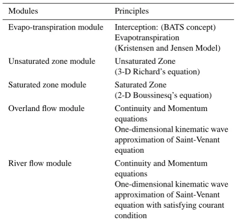
The interception and evapotranspiration simulation mod-ule estimates total loss of water by calculating intercepted water in leaf area, evaporated water from soil surface and transpirated water from vegetation before rainfall generates runoff. The model uses BATS concept and Kristensen and Jensen Model for estimating interception and Evapotran-spiration, respectively. The unsaturated zone module sim-ulates the movement of water considering soil infiltration rate and soil moisture content in root zone using three-dimensional Richard’s equation. Saturated zone module uses two-dimensional Boussinesq’s equation to simulate the sub-surface water flow where all the voids in soil are filled with water. Overland flow simulation module solves the hydrolog-ical parameters in each land grid and estimates the amount of lateral flow discharging into the river systems. The channel network flow simulation module calculates hydrological pa-rameters in each river nodes considering hydraulic parame-ters associated with flow path and the lateral flow coming to river systems from surface area. The principles of different modules are summarized in Table 1.

Although the model is capable of simulating back water effect using two-dimensional and one-dimensional diffusive wave approximations of the Saint-Venant continuity and mo-mentum equations at surface and river areas, respectively, a one-dimensional kinematic wave approximation can also be suitably applied in this model at both areas when the flow is unidirectional and back water effect is insignificant. In that case, the model simulates surface and river flow movements based on the direction of steepest descent among the eight adjacent cells. The kinematic wave approximation reduces computational time considerably and is efficient when sim-ulating large scale river basin incorporating other modules

Table 1. Principles of DHM (Dutta et al., 2000).

Modules Principles

Evapo-transpiration module Interception: (BATS concept) Evapotranspiration

(Kristensen and Jensen Model) Unsaturated zone module Unsaturated Zone

(3-D Richard’s equation) Saturated zone module Saturated Zone

(2-D Boussinesq’s equation) Overland flow module Continuity and Momentum

equations

One-dimensional kinematic wave approximation of Saint-Venant equation

River flow module Continuity and Momentum equations

One-dimensional kinematic wave approximation of Saint-Venant equation with satisfying courant condition

along with watershed hydrology. The different modules in the adopted distributed hydrological model were developed by using FORTRAN programming language for computer simulation.

2.2 Sediment dynamic modules

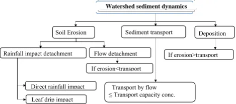
The sediment modules include sediment processes such as, soil erosion, sediment transport and deposition, with the driv-ing hydrological components. The modules represent soil erosion by estimating soil detachment due to raindrop im-pact and the shearing force of flowing water on the basis of established physical equations. Rainfall impacts are catego-rized into direct rainfall impact and leaf drip impact. Sedi-ment transport is simulated by using the governing equations of conservation of mass and momentum and a concept of transport capacity concentration. Soil detachments by flow and sediment deposition are estimated using the concept of transport capacity concentration. The concept of the process-based watershed sediment dynamics is shown in Fig. 1.

1310 M. A. Kabir et al.: Process-based distributed modeling approach for analysis of sediment dynamics

Watershed sediment dynamics

1 2

3

4 5

6

Fig. 1. Process-based approach of watershed sediment dynamics (after Foster, 1982).

Fig. 2. Structure of the process-based sediment dynamic model.

Data read DHM Start

Interception and ET simulation Unsaturated Zone

Simulation

DHM End Saturated Zone

Simulation Overland flow simulation River flow simulation

Data read for sediment modeling

Rainfall impact detachment simulation Overland flow detachment/ deposition simulation

River sediment detachment/ deposition simulation Output

Runoff Coe (RC) Rainfall impact detachment

Sediment transport Deposition

Direct rainfall impact Leaf drip impact

Flow detachment

Transport by flow

≤ Transport capacity conc. If erosion<transport

Soil Erosion

If erosion>transport

26

Fig. 1. Process-based approach of watershed sediment dynamics (after Foster, 1982).

sediment budgeting in a catchment (Atkinson, 1995; Ferro and Porto, 2000). Thus, the river and hillslope sediment dy-namics have been modelled separately.

In this modeling approach, hillslope soil detachment by rainfall impact is estimated using the kinetic energy delivered by rainwater when raindrops strike soil particles during a storm event. This kinetic energy is considered to be different for direct rainfall impact and leaf drip impact. Brandt (1989) derived an equation using rainfall intensity to calculate the kinetic energy for direct rainfall impact (Eq. 1). Relating canopy height to kinetic energy for leaf drip impact condi-tions, Brandt (1990) also proposed a relationship as shown in Eq. (2). The total Kinetic energy then can be described by Eq. (3).

KE(DT) = 8.95+8.44log(I ) (1) KE(LD) = 15.8(PH)0.5−5.87 (2) KE = KE(DT)·(1−CC)·HTotal+KE(LD)·CC·HNet (3)

Where, KE (DT) and KE (LD) is the kinetic energy in J m−2mm−1for direct rainfall impact and leaf drip impact conditions, respectively. HNet is the depth of net rainfall in

mm which is estimated by deducting the interception loss of water from the depth of total rainfall (HTotalin mm).Iis the

rainfall intensity in mm h−1and PH is the canopy height in m. The total KE in J m−2is calculated by introducing canopy coverage factorCCas shown in Eq. (3). TheCCis estimated

from land use data on a scale of 0.0 to 1.0; 0 for bare land and 1.0 for highly dense forest area.

Torri et al. (1987) related total kinetic energy to the amount of detached soils by rainfall impact as shown in Eq. (4). DR = k

ρs

(KE)e−Zh (4)

Where, DR is the soil detachment by rainfall impact in m3s−1m−1,kis the soil detachability index in g j−1,ρs is

the soil density in kg m−3,e−Zhis the correction factor for water ponding whereZdepends on soil texture, typical value lies in-between 0.9 to 3.9 andhis surface water depth in m.

The value of this correction factor decreases from 1.0 to to-wards 0.0 for the increase ofhfrom 0.0 m. Park et al. (1982) proposed an equation (Eq. 5) to estimate water ponding cor-rection factor to calculate soil detachment by rainfall impact using median raindrop diameter. The use of rainfall intensity and raindrop diameter relationship (Eq. 6) derived by Laws and Parsons (1943) as described in Jain et al. (2005) makes the latter mentioned water ponding correction factor easier to estimate.

FW=exp(1−h/Dm)ifh > Dm

=l ifh≤Dm

(5)

Dm=0.00124I0.182 (6)

Where,FW, as an alternative ofe−Zhin Eq. (4), is the water

depth correction factor ranging from 1.0 to 0.0,h is water depth in m,Dmis the raindrop diameter in m,I is the rainfall

intensity in mm h−1_.

Soil detachments by flow and sediment deposition are practically two mutually exclusive events. But, both the pro-cesses are considered to work on simultaneously in most of the modeling approaches. Flow detachment or deposi-tion can be expressed by Eq. (7) as described by Morgan et al. (1998) using the generalized erosion-deposition theory proposed by Smith et al. (1995). In this equation, transport capacity concentration (TC) is a baseline defined by a hypo-thetical concept which reflects a sediment concentration that balances the rate of erosion by flow and the accompanying rate of deposition.

DF = βSw vs(TC−CS) (7)

Where, DF is the flow detachment or deposition in m3s−1m−1for sediment concentration CS (m3m−3), wis

the width of the flow in m, νs is the particle settling

veloc-ity in m s−1andβS is a correction factor to calculate

cohe-sive soil erosion. In case of cohecohe-sive soil, cohesion force encounters detachment processes. Thus, βS is equal to 1.0

for non-cohesive soil detachment or any form of deposition but it decreases from 1.0 to towards 0.0 with high cohesive values of soil during detachment as shown in Eq. (8).

βs = 0.79e−0.85J (8)

M. A. Kabir et al.: Process-based distributed modeling approach for analysis of sediment dynamics 1311 Watershed sediment dynamics

1 2 3 4 5 6

Fig. 1. Process-based approach of watershed sediment dynamics (after Foster, 1982).

Fig. 2. Structure of the process-based sediment dynamic model.

Data read DHM Start Interception and ET simulation Unsaturated Zone Simulation DHM End Saturated Zone

Simulation Overland flow simulation River flow simulation

Data read for sediment modeling

Rainfall impact detachment simulation Overland flow detachment/ deposition simulation

River sediment detachment/ deposition simulation Output

Runoff Coe (RC) Rainfall impact detachment

Sediment transport Deposition

Direct rainfall impact Leaf drip impact

Flow detachment

Transport by flow

≤ Transport capacity conc. If erosion<transport

Soil Erosion

If erosion>transport

26

Fig. 2. Structure of the process-based sediment dynamic model.

from 2 to 100 cm3cm−1s−1(Morgan et al., 1998). Eq. (9) shows the expressions of Govers TC as mentioned in Mor-gan et al. (1998) in terms of a hydraulic variable named unit stream power (ω)andd50which were calibrated for any

par-ticle size ranging from 50 to 250 µm with maximum sediment concentrations up to 0.32 m3m−3.

TC=c (ω−ωcr)η;ω=10V s;c=[(d50+5)/0.32]−0.6;

η=[(d50+5)/300]0.25 (9)

Where, TC is the transport capacity in m3 m−3, ω is the unit stream power in cm s−1,V is the mean flow velocity in m s−1, s is the slope in percentage,ωcris the critical value

of unit stream power and the value is 0.4 cm s−1considered in Govers equation, cand ηare coefficients depending on median particle size,d50of the soil as in mum.

The sediment modules have been developed and inter-preted under FORTRAN programming environment to make compatible to the adopted distributed hydrological model and are incorporated as sub-components within the DHM en-vironment. The overall sediment dynamic model indicating different modules and their simulation sequence is shown in Fig. 2.

3 Solution scheme

The movement of sediments in each discretized cell is de-termined by associating them with water discharge based on the principle of conservation of mass and momentum sim-ilar to the flow simulation in the DHM as stated earlier. The one-dimensional kinematic wave approximation is ap-plied to simulate flow and sediment transport in both land grids and river nodes along the steepest descent direction. As sediment transport is primarily associated with flow, sed-iment transport estimation becomes much easier since cal-culation processes are set to be started just after the simula-tion of water discharge and head in land grids or river nodes within the same time interval. The backward finite-difference

1 2 3 4 5 6 7 8 9 10 11 12 13 14 15 16 17 18 19 20 21 22 23 24 25

Fig. 3. Time and space derivatives of both Q and Cs by finite-difference scheme in kinematic modeling (after Chow, 1959).

Fig. 4. Solution approaches for flow and sediment transport in distributed areas (description shown in Table 3).

Known value of Q, CS

Unknown value of Q, CS

Distance x

Time t t Δ x Δ x

iΔ ( )i+1Δx

(j+1)Δt

t jΔ x Q ∂ ∂ t Q ∂ ∂ CS ∂ x ∂ t CS ∂ ∂ ( 1 1 + + j i Q )1 1 + + j i S C j i Q+1

( )j+1

i S C 1 1 + + j i Q S q

( )j i S C j i Q 1 + j i Q

( )j i S C +1

Q q

( ) ( ) j i j i S j i

S Q Q

C +1= +1/ +1

54 6 0 1 0 0 0 0

0 59 3 0 1 2 1 0

2 61 0 0 5

3

0 0

0 66

0 0 12 0 0 0

0 0 69 14 0 0 1 1

3 0 71 16 1 0 2 2

2 4 0 89 4 1 3 3

3 5 0 92 6 0 4 4

11 6 0 0 101 0 5 5

670 683 685 687 790 0 6 13

4 7 8 9 10 803 804 838

1 1 17 19 23 24 32 0

0 0 16 0 2 4 0 4

3 0 15 0 0 3 1 3

(a)

(b)

(c)

(d) Flow accumulation from Flow direction map based

on Eight-direction pour point algorithm

( )j1 1 i S C , Q ++

2 S 2,C

Q

{Q,CS}( )np1

{Q,CS}( )np2 1 S 1,q

q

(CS,Q)b3

( )j1 1 i S,Q

C ++

(CS,Q)b1

(CS,Q)b2

2 2 S ,q

q ( )j1

i S,Q

C +

1 S 1,C

Q

27 Fig. 3. Time and space derivatives of bothQ and Cs by

finite-difference scheme in kinematic modeling (after Chow, 1959).

scheme has been taken into consideration in solving kine-matic wave equations numerically. The approximations of time and space derivatives of flow (Q) and sediment concen-tration (Cs)on x-t grid are shown in Fig. 3. The kinematic

wave equations and their finite-difference interpretations are presented in Table 2. The meaning of different symbols used is appended at the end.

1312 M. A. Kabir et al.: Process-based distributed modeling approach for analysis of sediment dynamics

Table 2. Kinematic wave equations and finite difference interpretation.

Equations for solution of “Q” Equations for solution of “CS”

∂Q

∂x+αβQ

β−1∂Q

∂t =q

Where,A=

nP2/3

s1/2

3/5

Q3/5=α Qβ

Qj_i++11−Q

j+1

i

1x +αβ

Qj_i+1+Q

j+1

i

2

β−1

Qj_i++11−Q

j i+1

1t =

q_ij++11−q

j i+1 2

∂QS

∂x +

∂AS

∂t −e(x,t )=qS

Where,QS=Q CS;Q=AV;QS=ASV

∂(QCS)

∂x +

∂QCS

V

∂t −e(x,t )=qS, e(x,t )=DR+DF

(QCS)j

+1

i+1−(QCS)j

+1

i

1x +

_QC

S

V

j+1

i+1

−QCS

V

j i+1

1t −[e(x,t )]

j+1

i+1=

(qS)j

+1

i+1−(qS)ji+1 2

Table 3. Solution approaches for flow and sediment transport in distributed areas (as described in Fig. 4).

Components Flow simulation Sediment simulation

(a) Land grids (Q1+Q2) RF

→Qj_i++₁1 Q1CS1+Q2CS2

Q1+Q2

_DR+DF → (CS)j

+1 i+1

Qj_i++₁1=

" 1t 1xQ

j+1 i +αβ

Qj_i+1+Qj_i+1 2

β−1

Qj_i+1+1t

q_ij₊+₁1+q_ij₊₁ 2

#," 1t 1x+αβ

Qj_i+1+Qj_i+1 2

β−1#

(CS)j

+1 i+1=

21t 1x (DR+βSw vST C)+1t 1x βSwvS(CS)ji+1+

21xQj_i+1(CS)ji+1

V_ij+1

+21t Qj_i+1(CS)j

+1 i

21x Qj_i++11

V_ij++11

+21t Qj_i++₁1+1t 1xβ_Sw v_S

(b) Lateral flow to river q=q1+q2=Qj

+1 i+1−Q

J+1

i qS=qS1+qS2=Q j+1 i+1(CS)

j+1 i+1−Q

J+1 i (CS)

j+1 i −DF

(c) River nodes Q(np1) q→Q(np2) CS(np1) qS

→ +DFCS(np2)

Q(np2)=

1t

1xQ(np1)+αβ

P Q(np2)+Q(np1) 2

β−1

P Q(np2)+1t

q(np2)+p q(np2) 2

1t 1x+αβ

_{P Q(np2)+Q(np1)}

2

β−1

CS(np2)=

h

21t 1x (βSwvST C)+1t 1xβSwvSCS(np1)+21x P Q(npP V (np2)P2)CS(np2)+21t Q(np1)CS(np1) +1t 1xqs(np2)

1x +

p qs(np2)

1x

i.h_{21x Q(np2)}

V (np2) +21t Q(np2)+1t 1xβSwvS i

(d) Confluence points at rivers Qb3=Qb1+Qb2 (CS)b3=Qb1(CS)b1

+Qb2(CS)b2

Qb1+Qb2

4 Model applications

The model has been tested on two different hydro climatic areas in Japan (Abukuma River Basin) and in Australia (La-trobe River Basin). These two study areas are distinct in terms of rainfall, slope and water discharge as shown in Ta-ble 4. Higher average slopes in Abukuma River Basin result in a low time of concentration in comparison with Latrobe River Basin. Abukuma River Basin also experiences higher rainfall than Latrobe River Basin. The two different hydro climatic areas have been chosen as study areas to analyze the applicability of the model in different regions.

Table 4. Characteristics of the study areas.

Study areas Annual avg. Avg. Slope Max. daily avg.

RF (mm) in % Q (m3_s−1₎

Abukuma River 1302.0 6.57 4804.25

Basin, Japan (in 2002) (in 2002 at Tateyama)

Latrobe River 975 4.9 16.18

M. A. Kabir et al.: Process-based distributed modeling approach for analysis of sediment dynamics 1313 1 2 3 4 5 6 7 8 9 10 11 12 13 14 15 16 17 18 19 20 21 22 23 24 25

Fig. 3. Time and space derivatives of both Q and Cs by finite-difference scheme in kinematic

modeling (after Chow, 1959).

Fig. 4. Solution approaches for flow and sediment transport in distributed areas (description

shown in Table 3).

Known value of Q, CS

Unknown value of Q, CS

Distance x

Time t t Δ x Δ x

iΔ ( )i+1Δx

(j+1)Δt

t jΔ x Q ∂ ∂ t Q ∂ ∂ CS ∂ x ∂ t CS ∂ ∂ ( 1 1 + + j i Q )1 1 + + j i S C j i Q+1

( )j+1

i S C 1 1 + + j i Q S q

( )j i S C j i Q 1 + j i Q

( )j i S C +1

Q q

( ) ( ) j i j i S j i

S Q Q

C +1= +1/ +1

54 6 0 1 0 0 0 0

0 59 3 0 1 2 1 0

2 61 0 0 5

3

0 0

0 66

0 0 12 0 0 0

0 0 69 14 0 0 1 1

3 0 71 16 1 0 2 2

2 4 0 89 4 1 3 3

3 5 0 92 6 0 4 4

11 6 0 0 101 0 5 5

670 683 685 687 790 0 6 13

4 7 8 9 10 803 804 838

1 1 17 19 23 24 32 0

0 0 16 0 2 4 0 4

3 0 15 0 0 3 1 3

(a)

(b)

(c)

(d)

Flow accumulation from Flow direction map based on Eight-direction pour point algorithm

( )j1 1 i S

C , Q ++

2 S 2,C

Q

{Q,CS}( )np1 {Q,CS}( )np2

1 S 1,q

q

(CS,Q)b3

( )j1 1 i S,Q

C ++

(CS,Q)b1

(CS,Q)b2 2

2 S,q

q ( )j1

i S,Q

C +

1 S 1,C

Q

27

Fig. 4. Solution approaches for flow and sediment transport in dis-tributed areas (description shown in Table 3).

# The following figures need to be replaced with their captions provided below:

Page 7:

55% 14%

16%

(a) (b)

Fig. 5. Abukuma River Basin location in Japan and land use map.

Page 7:

(a) DEM (b) Flow accumulation map

Fig. 6. Spatial data over view for Abukuma River Basin modelling. Fig. 5. Abukuma River Basin location in Japan and land use map.

4.1 Study area 1 (Abukuma River Basin, Japan)

Abukuma is the 6th longest river in Japan and starts from the Nasu Mountains in Tohoku region. The river flows mostly northwards throughout the basin areas and ultimately drains into the Pacific Ocean near the city of Kakuda (Fig. 5a). The river basin is about 5390 km2covered by mainly forest ar-eas (Fig. 5b) with the main stream of 234 km in length. The basin sustains a population of 1.2 million and comprises ma-jor cities such as Shirakawa, Sukagawa, Koriyama, Nihon-matsu, Fukushima, Kakuda, etc. Abukuma River also con-sists of many tributaries and has very steep gradients in many locations.

# The following figures need to be replaced with their captions provided below:

Page 7:

55% 14%

16%

(a) (b)

Fig. 5. Abukuma River Basin location in Japan and land use map.

Page 7:

(a) DEM (b) Flow accumulation map

Fig. 6. Spatial data over view for Abukuma River Basin modelling. Fig. 6. Spatial data overview for Abukuma River Basin modelling.

4.1.1 Model setup

The model has been set up to simulate a flood event occurred in July 2002 at Abukuma River Basin, Japan. Only measured daily water discharge data is available throughout the period. Measured hourly water and sediment flow data is available in flood peak hours. The digital elevation model (DEM) of 500-m grid spacing has been used in simulation as shown in Fig. 6a, which was generated from 50-m resolution point ele-vation data. Figure 6b shows flow accumulation map, which has been derived from the DEM using the eight-direction pour point algorithm (Jenson and Domingue, 1988). The river network that has been used for simulation is also shown in the same figure, where Tateyama and Fukushima are the two river gauging stations selected for model calibration and verification. The river network was delineated from flow ac-cumulation map by choosing the threshold values for channel initiation. The sub-catchments near the Pacific Ocean have not been considered in this kinematic wave simulation since those areas are subjected to tidal effects.

1314 M. A. Kabir et al.: Process-based distributed modeling approach for analysis of sediment dynamics Page 8:

(a) At Tateyama (b) At Fukushima

Fig. 7. Daily avg. water and suspended sediment discharge.

Page 8:

(a) At Tateyama (b) At Fukushima

Fig. 8. Correlation of observed and simulated daily avg. water discharge (N = number of observations)

Fig. 7. Daily avg. water and suspended sediment discharge.

Page 8:

(a) At Tateyama (b) At Fukushima

Fig. 7. Daily avg. water and suspended sediment discharge.

Page 8:

(a) At Tateyama (b) At Fukushima

Fig. 8. Correlation of observed and simulated daily avg. water discharge (N = number of observations)

Fig. 8. Correlation of observed and simulated daily avg. water dis-charge (N= number of observations).

highly related to soil texture. The theoretical range of values for soil detachability index is 0.01 to 10 g j−1, where maxi-mum values for sand and minimaxi-mum values for clay (Gumiere et al., 2009; Morgan et al., 1998; Morgan, 2001).

4.1.2 Simulations and discussion

The basin is highly sensitive to rainfall for flood discharge in river systems. The basin generates a high rate of overland flow due to hilly topography as well as to have a low time of concentration. The water budget distributions at Abukuma River Basin in July 2002 are revealed as 70.05% of overland flow, 26.57% of infiltration, 3.38% of interception and evap-otranspiration through simulations of different hydrological processes.

Figure 7a, b shows the simulated results of the average daily water and suspended sediment (SS) discharge together with the observed data at Tateyama and Fukushima river gauging stations and the basin average rainfall. Based on available measured data, it is found that the model has sim-ulated well the daily average flood water discharge at these

Table 5. Performance evaluation of hydrological and sediment modeling.

Items Stations Nash-Sutcliffe’s COE of

COE determination

Avg. daily,Q Tateyama_Fukushima 0.986_0.969 0.985_0.971

Hourly,Q Tateyama 0.843 0.931

Hourly,Qs Tateyama −4.26 −7.79

(Qs>2 m3s−1₎

Hourly,Qs Tateyama 0.88 0.87

(Qs<2 m3s−1)

two gauging stations. The correlation coefficients (R2 val-ues) are 0.985 and 0.971 between daily average observed and simulated water discharge at Tateyama and Fukushima sta-tions, respectively as shown in Fig. 8. Table 5 shows that a high Nash-Sutcliffe’s coefficients of 0.986 and 0.969 are also between simulated and observed daily average flows at these two stations, respectively. The simulated daily suspended sediment (SS) discharge data were not shown here with the observed value due to the unavailability of data in the daily scale. However, the simulated daily average suspended sedi-ment (SS) discharge follows a similar trend as water flows in both stations.

M. A. Kabir et al.: Process-based distributed modeling approach for analysis of sediment dynamics 1315

Page 9:

Fig. 9. Hourly water discharge at Tateyama station (11 July 2002).

Page 9:

Fig. 10. Correlation of observed and simulated hourly water discharge at Tateyama (11 July 2002) (

N

= number of observations)

Page 9:

Fig. 11. Hourly suspended sediment discharge at Tateyama station (11 July 2002).

Page 9:

Fig. 9. Hourly water discharge at Tateyama station (11 July 2002).

Page 9:

Fig. 10. Correlation of observed and simulated hourly water discharge at Tateyama (11 July 2002) (

N

= number of observations)

Page 9:

Fig. 11. Hourly suspended sediment discharge at Tateyama station (11 July 2002).

Fig. 10. Correlation of observed and simulated hourly water dis-charge at Tateyama (11 July 2002) (N= number of observations).

the observed and simulated results of hourly water discharge during peak flood hours on 11 July 2002 at Tateyama sta-tion. The simulation performance for hourly simulated water discharge is also found to be reasonable good with a corela-tion coefficient (R2value) of 0.931 as shown in Fig. 10. Ta-ble 5 also shows a high Nash-Sutcliffe’s Coefficient of 0.843 in the same comparison. High resolution spatial data is re-comended for further improvement of simulation results at peak points.

The model has also well-simulated hourly suspended sed-iment (SS) discharge except during flood peak hours. Fig-ure 11 shows observed and simulated hourly SS discharge with flow velocity at Tateyama station. There is a close match between the model results and the observed data when the SS discharge is lower than 2.0 m3s−1. Figure 12 shows that the correlation value (R2value) between observed and simu-lated SS discharge is 0.87 when SS discharge is less than 2.0

Page 9:

Fig. 9. Hourly water discharge at Tateyama station (11 July 2002).

Page 9:

Fig. 10. Correlation of observed and simulated hourly water discharge at Tateyama (11 July 2002) (N

= number of observations)

Page 9:

Fig. 11. Hourly suspended sediment discharge at Tateyama station (11 July 2002). Fig. 11. Hourly suspended sediment discharge at Tateyama station (11 July 2002).

Fig. 9. Hourly water discharge at Tateyama station (11 July 2002). 1

2

3 4

Fig. 10. Correlation of observed and simulated hourly water discharge at Tateyama station (11 July 2002) (N= number of observations).

0 2 4 6 8 10

0 1 2 3 4 5

150 200 250 300 350 400

Ho

u

rly

Qs

(m

3/s

)

Time (hrs)

Sim Qs Obs Qs Vel. V

Ho

u

rly

V

elo

ci

ty

(m/s

)

5

6

7 8

Fig. 11. Hourly SS discharge at Tateyama station (11 July 2002).

(a) Qs > 2 m3_{/s (b) Qs < 2 m}3_/s

30 Fig. 12. Correlation of observed and simulated hourly suspended

sediment discharge at Tateyama station (N= number of observa-tions).

m3s−1and it reveals a very poor relation when SS discharge is more than 2.0 m3s−1(Table 5). The Nash-Sutcliffe’s co-efficient of simulated SS discharge in comparison with ob-served SS discharge less than 2.0 m3s−1_{is also high (0.88)}

(Table 5).

As described earlier, the Govers transport capacity equa-tion has been applied to simulate suspended sediment trans-port in these model applications. It is worth mentioning that this transport capacity equation is based on unit stream power and median grain size (d50)values in limited conditions. The

method considers an experimentally evaluated constant crit-ical value of unit stream power to simulate suspended sed-iment transport. In this method, the recommended particle size ranges from 0.05 to 0.25 mm under the low flow condi-tions that are usually observed at rill locacondi-tions. The transport capacity in Govers equation is less sensitive to flow veloc-ity and slope of the basin. With these conditions, suspended sediment discharge in river systems is found to be reasonably consistent with channel flow as expected.

1316 M. A. Kabir et al.: Process-based distributed modeling approach for analysis of sediment dynamics On the other hand, grains smaller than 0.125 mm always

behave as suspended sediment usually while grains coarser than 8.0 mm travel as bed load (Wilcock, 2004). There is no unique grain size in representing the boundary of these two loads since the processes are highly variable with flow strength. The flow at Tateyama exerted a higher degree of forces to river bed during peak flood hours on 11 July 2002 which increased suspended sediment ranges towards 8.0 mm, far exceeding Govers threshold limit of 0.25 mm. Therefore, the simulated suspended sediment values were found to be smaller than the observed value. Analyses considering sedi-ment size class seperately with determining respective shear stress based transport capacity are recommended for simulat-ing river sediment dynamics at high flow conditions.

4.1.3 Sensitivity analysis

A parametric study has also been carried out before the cali-bration. Soil particle size and density effects have been anal-ysed since sediment transport involves the movement of dif-ferent types of soil particles having large variability in both size and density (Nord et al., 2009). The effect of soil cohe-sion has also been investigated since it reflects the contribu-tion of plant roots in soil detachment and the variacontribu-tion of top soil erodibility (Baets at el., 2008). In the calibrated condi-tion, the soil density was considered as 2480 kg m−3_on

aver-age irrespective of the soil and land use classifications due to simplification of the problem. The ranges of particle sizes in terms ofd50and soil cohesions were 75 to 125 µm and 4.5 to

5.0 kPa, respectively in the calibrated condition. It is worth noting here that the soil particle size, density and cohesion have been considered based on the limited point sampling data mostly at Tateyama station.

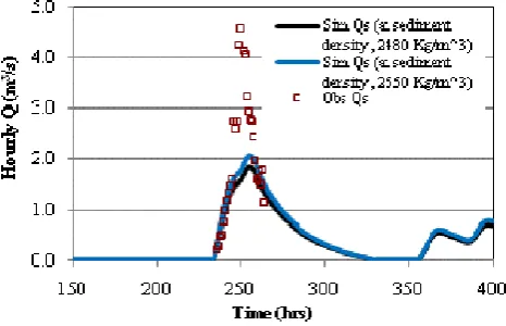
Figure 13 shows simulated suspended sediment discharge (Qs) in Abukuma River Basin at Tateyama station for

two different soil densities with the observed one during July 2002. It revealed that the peak of suspended sediment discharge (Qs) has increased by 11.40% for soil density

2650 kg m−3 _{in lieu of 2480 kg m}−3_{. Suspended sediment}

discharge (Qs)during peak hour of July 2002 is found to be

increased by 15.56% and decreased by 14.79% due to the in-crease and dein-crease ofd50value in each soil class by 10%,

respectively as shown in Fig. 14. The suspended sediment discharge (Qs)is much sensitive with soil cohesion since a

decrease of soil cohesion implies an increase of soil erodibil-ity and a less effect of vegetation’s encountering to soil ero-sion. Figure 15 shows that the peaks of suspended sediment discharge (Qs)increase by 20.91% and decrease by 17.32%

due to the decrease and increase of soil cohesion value by 5%, respectively during same period.

Page 10:

Fig. 13. Qs with different soil densities at Tateyama station.

Page 10:

Fig. 14. Qs with different d

values at Tateyama station.

Fig. 13.Qswith different soil densities at Tateyama station.

Page 10:

Fig. 13. Qs with different soil densities at Tateyama station.

Page 10:

Fig. 14. Qs with different d

values at Tateyama station.

Fig. 14.Qswith different d50 values at Tateyama station.

4.2 Study area 2 (Latrobe River Basin, Australia)

Latrobe River Basin is located in south-eastern part of Vic-toria, Australia as shown in Fig. 16. The main stream of this watershed is Latrobe River, which flows eastwards through-out the whole basin and ultimately discharges into Lake Wellington. The central part of this basin is low elevated and covered with elongated flat farmland with unconsoli-dated soils, which are very much sensitive to bank erosion (DPI, 2009). The other parts excluding central region con-sist of steep mountains with fairly dense forest. The basin includes the three major towns of Moe, Morwell and Trar-algon along its central part. The total basin area is around 4,675 km2 and it sustains a population of 97 339 (BRS and BOM, 2008).

4.2.1 Model setup

M. A. Kabir et al.: Process-based distributed modeling approach for analysis of sediment dynamics 1317 Page 11:

Fig. 15. Qs with different soil cohesion values at Tateyama station.

Page 12:

Fig. 18. Water discharges at Rosedale with basin avg. rainfall (ML=Mega liters). Fig. 15.Qswith different soil cohesion values at Tateyama station.

0 1 2 3 4 5

150 200 250 300 350 400

Ho

u

r

ly

Q

(m

^

3

/s

)

Time (hrs)

Sim Qs (at soil cohesion ranges 4.5 to 5.0 kPa) Sim Qs (Soir cohesion decreased by 5%) Sim Qs (Soir cohesion increased by 5%) Obs Qs

1

2

3

4

5

6

Fig. 15.QS with different soil cohesion values at Tateyama station.

Western Australia

Northern

South

Queensland

New South Wales

ACT Victoria

Tasmania

Latrobe River basin

Fig. 16. Latrobe River Basin location in Victoria, Australia.

32 Fig. 16. Latrobe River Basin location in Victoria, Australia.

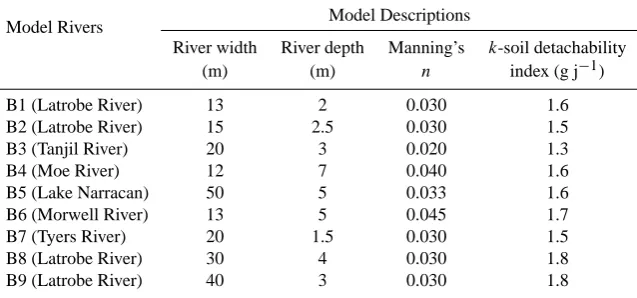
river network which have been generated from SRTM DEM are shown in Fig. 17a. Rosedale, Scarnes Bridge and Thoms Bridge are three gauging stations along the river network, which have been selected for calibration and verification of the model application. The maximum temporal resolution has also been set to 1-h during model simulation. Similar to Abukuma River Basin modeling, roughness coefficient (n) values and an index of soil detachability (k)have been con-sidered main calibrating parameter in this case study. The major river network has been described in terms of hydraulic parameters associated with each of river branches to cap-ture river flow dynamics properly. The different branches of Latrobe River have been named separately in this study as shown in Fig. 17b. Table 6 describes the hydraulic param-eters of different river branches including calibrating terms that have used in model simulation.

1 2

3

4 5

6

7

8

9

(a) (b)

Fig. 17. Flow accumulation map and river network for Latrobe River Basin modeling.

Fig. 18. Water discharge at Rosedale with basin avg. rainfall (ML=Mega liters).

33

Fig. 17. Flow accumulation map and river network for Latrobe River Basin modeling.

4.2.2 Simulations and discussion

The total water budget allocation during 2007 flood periods (June to August) based on simulation results of different hy-drological modules is 48.47% of infiltration, 39.42% of in-terception and evapotranspiration, 12.11% overland flow. It implies that a higher interception and evapotranspiration rate in Latrobe River Basin minimizes the amount of overland flow into the river systems. In 2007, the flood hydrographs in different stations revealed multiple peaks during June to August. Figure 18 shows observed and simulated results of water discharge at Rosedale points with basin average rain-fall. The simulated results show much higher values in com-parison with observed values during first flood peak hours. This is not surprising since the basin has a high soil mois-ture capacity that triggers a high infiltration rate (Potter et al., 2005) and the flooding conditions had started in this case just after a long dry spell. The actual runoff coefficient had significantly lower at that time than the constant or average runoff coefficient of the entire flood season. It has revealed that a runoff coefficient of 0.2 allocates water distributions properly for hydrological simulations at Latrobe River Basin when the basin antecedent soil moisture content is high.

1318 M. A. Kabir et al.: Process-based distributed modeling approach for analysis of sediment dynamics

Table 6. efinition of Latrobe River Branches for model simulation.

Model Rivers Model Descriptions

River width River depth Manning’s k-soil detachability

(m) (m) n index (g j−1)

B1 (Latrobe River) 13 2 0.030 1.6

B2 (Latrobe River) 15 2.5 0.030 1.5

B3 (Tanjil River) 20 3 0.020 1.3

B4 (Moe River) 12 7 0.040 1.6

B5 (Lake Narracan) 50 5 0.033 1.6

B6 (Morwell River) 13 5 0.045 1.7

B7 (Tyers River) 20 1.5 0.030 1.5

B8 (Latrobe River) 30 4 0.030 1.8

B9 (Latrobe River) 40 3 0.030 1.8

Page 11:

Fig. 15. Qs with different soil cohesion values at Tateyama station.

Page 12:

Fig. 18. Water discharges at Rosedale with basin avg. rainfall (ML=Mega liters).

Fig. 18. Water discharge at Rosedale with basin avg. rainfall (ML = Mega liters).

Table 7. Performance evaluation of hydrological modeling at La-trobe River Basin.

Items No. of obs. Stations Nash-Sutcliffe COE

Avg. daily,Q

29 Rosedale 0.926

29 Scarnes Br. 0.830

29 Thoms Br. 0.818

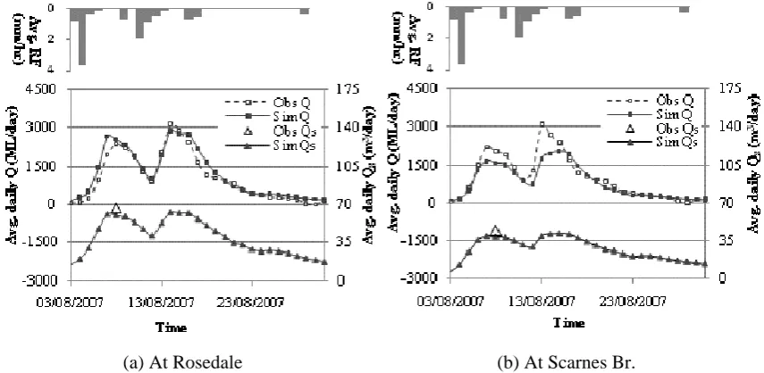
The suspended sediment discharge at Rosedale and Scarnes Br. is found to follow a similar trend as on the wa-ter discharge along the river channels. A relatively smaller

Table 8. Performance evaluation of suspended sediment modeling at Latrobe River Basin.

Items Date of obs. Stations % of deviation at single obs. Avg. daily,Qs 08/08/2007 Rosedale +9.73

08/08/2007 Scarnes Br. +12.3

portion from eroded soils from hillslope area reaches to the river systems due to less overland flow. On the other hand, many reservoirs along the river courses caused a decrease of flow velocity which promotes deposition of sediments of large particle sizes. Analyses of observed data revealed that the water discharge at Latrobe River delivered a limited force to channel systems during the flood events in August 2007 and in these circumstances, the suspended sediment con-centration ranges were within the threshold limits of using the Govers transport capacity equation as discussed earlier. Therefore, simulated suspended sediments at different river gauging stations are found to be reasonable (less than 15% deviation) by comparing with a single observed data as de-scribed in Table 8.

5 Conclusions

M. A. Kabir et al.: Process-based distributed modeling approach for analysis of sediment dynamics 1319 Page 13:

(a) At Rosedale (b) At Scarnes Br.

Fig. 19. Water and suspended sediment discharge with basin avg. rainfall (ML = Mega liters). Fig. 19. Water and suspended sediment discharge with basin avg. rainfall (ML = Mega liters).

1

2 3

4

0

2

4

Av

g. RF

(m

m

/h

r)

0

2

4

Avg

. R

F

(mm/

hr)

(a) At Rosedale (b) At Scarnes Br.

Fig. 19. Water and suspended sediment discharge with basin avg. rainfall (ML=Mega liters).

5 6

7 8

(a) At Rosedale (b) At Scarnes Br.

Fig. 20. Correlation of observed and simulated water flow at Latrobe River (N= number of

observations, ML=Mega liters).

34

Fig. 20. Correlation of observed and simulated water flow at La-trobe River (N= number of observations, ML = Mega liters).

of flowing water whereas movements of flow and sediment particles are calculated using a backward finite difference algorithm based numerical solution of the kinematic wave approximation of the Saint-Venant equations. The Gov-ers (1990) transport capacity equation and a set of constant runoff coefficients have been used in the model applications. The model has well simulated runoff at Abukuma River Basin, Japan with highest and lowest Nash-Sutcliffe’s coef-ficients of 0.986 and 0.843, respectively at the different river gauging stations during the flood event of July 2002. The model has also satisfactorily calculated suspended sediment transport in the basin at low flow conditions. The correlations 0.515 and 0.780 using Nash-Sutcliffe efficiency andR-squar value, respectively have been found at Tateyama station with suspended sediment discharge less than 2.0 m3_s−1_{. This was}

expected due to the limitation associated with using Govers transport capacity equation at high flow conditions.

The Latrobe River Basin is highly dependent on the soil moisture antecedent conditions and thus, the simulation of July 2007 flood using a constant runoff coefficient gave er-roneous results since the flood occurred just after a long dry spell. The model has performed well in simulating runoff at Latrobe River Basin, Australia with highest and lowest Nash-Sutcliffe’s coefficient of 0.93 and 0.82, respectively at different river gauging stations during the flood event Au-gust 2007. Based on the limited observed data, the model has also been found to be consistent in estimating suspended sediment transport in the two river systems.

1320 M. A. Kabir et al.: Process-based distributed modeling approach for analysis of sediment dynamics Appendix A

A list of symbols used in this paper

Symbol Meaning Unit

βs Correction factor for cohesive soil erosion –

ρs Soil density kg m−3

ω Channel stream power cm s−1

ωcr Critical stream power cm s−1

1x,1t Spatial, temporal intervals meter, s

c,η Coefficient related to particle size –

A Water flow cross-section m2

As Cross-section of sediment flow m2

CC Canopy coverage factor –

Cs Sediment concentration m3m−3

d50 Median grain size µm

Dm Raindrop diameter meter

DF Flow detachment or deposition m3_s−1_m−1

DR Soil detachment by rainfall m3_s−1_m−1

h Depth of water meter

Hnet Net rainfall depth mm

HTotal Total rainfall depth mm

I Rainfall intensity mm h−1

i,j Spatial, temporal points –

J Soil torvane shear strength kPa

k Soil detachability index g j−1

KE (DT) Kinetic energy due to direct rainfall j g−1_mm−1

KE (LD) Kinetic energy due to leaf drip j g−1mm−1

KE Kinetic energy j g−1

n Manning’s roughness –

N No. of observations –

np1, np2 Two consecutive river nodes –

P Wetted perimeter meter

PH Canopy height meter

q Later water discharges m2s−1

qs Lateral sediment flow m2s−1

Q Water discharge m3_s−1

Qs Sediment flow m3s−1

RF Rainfall mm h−1

s Land slope %

TC Transport capacity concentration m3_m−3

V Flow velocity m s−1

vs Particle settling velocity m s−1

W Water flow width meter

x,t Distance, time meter, s

Z Soil texture index –

P Q,P V,P Cs,P qs: Values ofQ,V,Cs,qsin previous

time intervals respectively

Acknowledgements. This project was funded by NEWJEC Inc.,

Japan and the small grant scheme of Monash University Gippsland Campus. The authors gratefully acknowledge the support. The three anonymous reviewers are acknowledged for their constructive criticism and valuable comments.

Edited by: M. Mikos

References

Aksoy, H. and Kavvas, M. L.: A review of hillslope and watershed scale erosion and sediment transport models, Catena, 64, 247– 271, 2005.

Apip, Tachikawa, Y., Sayama, T., and Takara, K..: Lumping a physically-based distributed sediment runoff model with embed-ding river channel sediment transport mechanism, Annuals of Disas. Prev. Res. Inst., Kyoto University, No. 51 B, 2008. Atkinson, E.: Methods for assessing sediment delivery in river

sys-tems, J. Hydrol. Sci., 40, 273–280, 1995.

Baets, S. D., Torri, D., Poesen, J., Salvador, M. P., and Meers-mans, J.: Modeling increased soil cohesion due to roots with EUROSEM, Earth Surf. Proc. Land., 33, 1948–1963, 2008. Beasley, D. B., Huggins, L. F., and Monke, E. J.: ANSWERS-A

model for watershed planning, T. ASAE, 23, 938–944, 1980. Bhattacharya, B., Price, R. K., and Solomatine, D. P.: Machine

learning approach to modeling sediment transport, J. Hydraul. Eng., 133, 440–450, 2007.

Bhattarai, R. and Dutta, D.: Estimation of soil erosion and sediment yield using GIS at catchment scale, J. Water Res. Manage., 21, 1635–1647, 2007.

Borah, D. K. and Bera, M.: Watershed-scale hydrologic and nonpoint-source pollution models: review of mathematical bases, T. ASAE, 46, 1553–1566, 2003.

Brandt, C. J.: The size distribution of throughfall drops under veg-etation canopies, Catena, 16, 507–524, 1989.

Brandt, C. J.: Simulation of size distribution and erosivity of rain-drops and throughfall rain-drops, Earth Surf. Proc. Land., 15, 687– 689, 1990.

Bureau of Rural Sciences (BRS) and Bureau of Meteorology (BOM).: Australia, July 2008 Latrobe River Basin Summary by CSIRO Online, http://adl.brs.gov.au/water2010/pdf/monthly reports/awap 226 report.pdf, last access: 1 April 2009, 2008. Chmelova, R. and Sarapatka, B.: Soil erosion by water:

contempo-rary research methods and their use, J. Geographica, 37, 23–30, 2002.

Chow, V. T.: Open channel flow, McGraw-Hill, New York, 294– 300, 1959.

Department of Primary Industries (DPI): Australia, A Guide to the Inland Angling Waters of Victoria, La Trobe River Basin, Online, available at: http://new.dpi.vic.gov.au/fisheries/ recreational-fishing/inland-angling-guide/?a=13398, last access: 14 April 2011, 2011.

Duna, S., Wua, J. Q., Elliot, W. J., Robichaudb, P. R., Flanaganc, D. C., Frankenbergerc, J. R., Brownb, R. E., and Xud, A. C.: Adapting the Water Erosion Prediction Project (WEPP) model for forest applications, J. Hydrol., 366, 46–54, 2009.

Dutta, D. and Nakayama, K.: Effects of spatial grid resolution on river flow and surface inundation simulation by physically based distributed modeling approach, J. Hydrol. Process, 23, 534–545, 2008.

Dutta, D., Herath, S., and Musiake, K.: Flood inundation simulation in a river basin using a physically based distributed hydrologic model, J. Hydrol. Process, 14, 497–519, 2000.

Ferro, V. and Porto, P.: Sediment Delivery Distributed (SEDD) model, J. Hydraul. Eng., 5, 411–422, 2000.

Fiener, P., Govers, G., and Oost, K. V.: Evaluation of a dynamic multi-class sediment transport model in a catchment under soil-conservation agriculture, Earth Surf. Proc. Land., 33(11), 1639– 1660, 2008.

M. A. Kabir et al.: Process-based distributed modeling approach for analysis of sediment dynamics 1321

Erosion Research Laboratory, 1995.

Foster, G. R.: Modeling the erosion process., in Hydrological mod-eling in small watersheds, edited by: Haan, C. T., Jonson, H., and Beakensiek, D. L., American Society of Agricultural Engineers, St. Joseph, MI, 297–380, 1982.

Foster, G. R. and Meyer, L. D.: Transport of soil particles by shal-low fshal-low, T. ASAE, 15, 99–102, 1972.

Govers, G.: Empirical relationships for the transport capacity of overland flow, in Erosion, transport and deposition processes, edited by: International Association of Hydrological Sciences, 189, 45–63, 1990.

Gumiere, S. J., Le Bissonnais, Y., and Raclot, D.: Soil resistance to interrill erosion: Model parameterization and sensitivity, Catena, 77, 274–284, 2009.

Hograth, W. L., Parlange, J. Y., Rose, C. W., Sander, G. C., Steen-huis, T. S., and Barry, A.: Soil erosion due to rainfall impact with inflow: an analytical solution with spatial and temporal effects, J. Hydrol., 2995, 140–148, 2004.

Huggins, L. F. and Monke, E. J.: The mathematical simulation of the hydrology of small watersheds, Technical Report 1, Purdue University Water Resources Research Center, 1966.

Jain, M. K., Kothyari, U. C., and Ranga Raju, K. G.: GIS Based Distributed Model for Soil Erosion and Rate of Sediment Out-flow from Catchments, J. Hydraul. Eng., 131, 755–769, 2005. Jenson, S. K. and Domingue, J. O.: Extracting topographic

struc-ture from digital elevation model data for geographic information system analysis, Photogramm. Eng. Rem. S., 54(11), 1593–1600, 1988.

Laws, J. O. and Parsons, D. A.: The relation of raindrop size to intensity, Transactions, American Geophysical Union, 24, 542– 460, 1943.

Merz, R., Bl¨oschl, G., and Parajka, J.: Spatio-temporal variability of event runoff coefficients, J. Hydrol., 331(3–4), 591–604, 2006. Morgan, R. P. C.: A simple approach to soil loss prediction: a revised Morgan-Morgan-Finney model, Catena, 44, 305–322, 2001.

Morgan, R. P. C., Quinton, J. N., and Rickson, R. J.: EUROSEM user guide version 3.1, Silsoe College, Cranfield University, Sil-soe, UK, 1993.

Morgan, R. P. C., Quinton, J. N., Smith, R. E., Govers, G., Poesen, W. A., Auerswald, K., Chisci, G., Torri, D., and Styczen, M. E.: The European Soil Erosion Model (EU-ROSEM): A dynamic approach for predicting sediment transport from fields and small catchments, Earth Surf. Proc. Land., 23, 527–544, 1998. Mughal, H.: Regional scale soil erosion and sediment transport

modeling, PhD Thesis, The University of Tokyo, Tokyo, 2001. Nearing, M. A., Foster, G. R., Lane, L. J., and Finkner, S. C.: A

pro-cess based soil erosion model for USDA water erosion prediction project technology, T. ASAE, 32, 1587–1593, 1989.

Noel, D. U.: A note on soil erosion and its environmental conse-quences in the United States, Water Air Soil Poll., 129, 181–197, 2001.

Nord, G., Esteves, M., Lapetite, J., and Hauet, A.: Effect of particle density and inflow concentration of suspended sediment on bed-load transport in rill flow, Earth Surf. Proc. Land., 34, 253–263, 2009.

Park, S. W., Mitchell, J. K., and Scarborough, J. N.: Soil erosion simulation on small watersheds: A modified ANSWERS model, T. ASAE, 25, 1581–1588, 1982.

Post, D. A., Waterhouse, J., Grundy, M., and Cook, F.: The past, present and future of sediment and nutrient modeling in GBR catchments, A summary of CSIRO workshop 2006, Brisbane, Australia, 7–12, 2007.

Potter, N. J., Zhang, L., Milly, P. C. D., McMahon, T. A., and Jakeman, A. J.: Effects of rainfall seasonality and soil moisture capacity on mean annual water balance for Australian catchments, Water Resour. Res., 41(6), W06007, doi:10.1029/2004WR003697, 2005.

Smith, R. E., Goodrich, D., and Quinton, J. N.: Dynamic dis-tributed simulation of watershed erosion: the KINEROS2 and EUROSEM models, J. Soil Water Conserv., 50, 517–520, 1995. Svoray, T. and Ben-Said, S.: Soil loss, water ponding and sediment

deposition variations as a consequence of rainfall intensity and land use: a multi-criteria analysis, Earth Surf. Proc. Land., 35, 202–216, 2010.

Torri, D., Sfalaga, M., and Del Sette, M.: Splash detachment: runoff depth and soil cohesion, Catena, 14, 149–155, 1987.