Hydrol. Earth Syst. Sci., 17, 3111–3125, 2013 www.hydrol-earth-syst-sci.net/17/3111/2013/ doi:10.5194/hess-17-3111-2013
© Author(s) 2013. CC Attribution 3.0 License.
EGU Journal Logos (RGB)
Advances in
Geosciences
Open Access
Natural Hazards
and Earth System
Sciences
Open AccessAnnales
Geophysicae
Open AccessNonlinear Processes
in Geophysics
Open AccessAtmospheric
Chemistry
and Physics
Open AccessAtmospheric
Chemistry
and Physics
Open Access DiscussionsAtmospheric
Measurement
Techniques
Open AccessAtmospheric
Measurement
Techniques
Open Access DiscussionsBiogeosciences
Open Access Open Access
Biogeosciences
Discussions
Climate
of the Past
Open Access Open Access
Climate
of the Past
Discussions
Earth System
Dynamics
Open Access Open Access
Earth System
Dynamics
DiscussionsGeoscientific
Instrumentation
Methods and
Data Systems
Open Access
Geoscientific
Instrumentation
Methods and
Data Systems
Open Access DiscussionsGeoscientific
Model Development
Open Access Open Access
Geoscientific
Model Development
DiscussionsHydrology and
Earth System
Sciences
Open AccessHydrology and
Earth System
Sciences
Open Access DiscussionsOcean Science
Open Access Open Access
Ocean Science
DiscussionsSolid Earth
Open Access Open Access
Solid Earth
Discussions
The Cryosphere
Open Access Open Access
The Cryosphere
DiscussionsNatural Hazards
and Earth System
Sciences
Open Access
Discussions
Inundation risk for embanked rivers
W. G. Strupczewski1, K. Kochanek1, E. Bogdanowicz2, and I. Markiewicz1
1Institute of Geophysics, Polish Academy of Sciences, Ksiecia Janusza 64, 01-452 Warsaw, Poland 2Institute of Meteorology and Water Management, Podlesna 61, 01-673 Warsaw, Poland
Correspondence to: W. G. Strupczewski ([email protected])
Received: 31 January 2013 – Published in Hydrol. Earth Syst. Sci. Discuss.: 8 March 2013 Revised: 13 June 2013 – Accepted: 24 June 2013 – Published: 2 August 2013
Abstract. The Flood Frequency Analysis (FFA) concentrates
on probability distribution of peak flows of flood hydro-graphs. However, examination of floods that haunted and devastated the large parts of Poland lead us to revision of the views on the assessment of flood risk of Polish rivers. It turned out that flooding is caused not only by the overflow of the levee crest but also due to the prolonged exposure to high water on levees structure causing dangerous leaks and breaches that threaten their total destruction. This is because the levees are weakened by long-lasting water pressure and as a matter of fact their damage usually occurs after the cul-mination has passed the affected location. The probability of inundation is the total of probabilities of exceeding em-bankment crest by flood peak and the probability of washout of levees. Therefore, in addition to the maximum flow one should also consider the duration of high waters in a river channel.
In the paper the new two-component model of flood dynamics: “Duration of high waters–Discharge Threshold– Probability of non-exceedance” (DqF), with the methodol-ogy of its parameter estimation was proposed as a completion to the classical FFA methods. Such a model can estimate the duration of stages (flows) of an assumed magnitude with a given probability of exceedance. The model combined with the technical evaluation of the probability of levee breaches due to the duration (d)of flow above alarm stage gives the annual probability of inundation caused by the embankment breaking.
The results of theoretical investigation were illustrated by a practical example of the model implementation to the series of daily flow of the Vistula River at Szczucin. Regardless of promising results, the method of risk assessment due to pro-longed exposure of levees to high water is still in its infancy despite its great cognitive potential and practical importance.
Therefore, we would like to point out the need for and useful-ness of the DqF model as complementary to the analysis of the flood peak flows, as in classical FFA. The presented two-component model combined with the routine flood frequency model constitutes a new direction in FFA for embanked rivers
1 Introduction
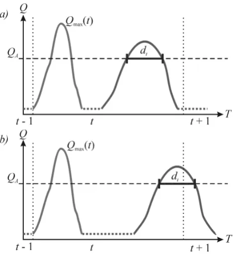
Fig. 1. Definition of the threshold flow discharge and duration in
DqF model: (a) the flood wave ofdtduration entirely in the yeart;
(b) the flood wave starts in the year t and continues int+1.
frequency of the annual maximum (AM) flows is not suitable in this case and ought to be supplemented by the analysis of the duration of flows over the given threshold (Bogdanowicz et al., 2011, also Eagleson, 1972; Sivapalan et al., 1990; Gioia et al., 2008; Iacobellis et al., 2011). The joint risk of inundation making allowance for the two main sources of vulnerability to flood hazard for areas protected by embank-ments, over-crest flow and levee failure, have been proposed and defined.
In Poland, as in many other countries for each hydrological station, two benchmark water levels, called the warning stage and the alarm stage, have been specified. Although warning and alarm stages are assigned to the places where water lev-els are observed, to the hydrological stations, their determi-nation procedures as well as other inundation risk character-istics take into account, inter alia, the elevation of the em-bankment system for the whole river reach. So, the results of below analysis refer to the river reaches represented by data observed at hydrological stations. The frequency of an-nual maximum uninterrupted duration,D(in days), of flows over the flood alarm stage (Fig. 1) can be used to assess the risk of flooding due to waning of the levees’ strength. The aim of this study is to introduce formal aspects of the duration–flow–frequency (DqF) modelling in stationary and non-stationary conditions, to use it to assess the inundation risk due to the levees breach and to combine it with the AM flow model to get the cumulative probability of inundation. In the presented statistical model, the duration is considered as
a random variable while the alarm flow discharge is the fixed value. The approach presented here for non-stationary condi-tions can to some extent resemble the Peak Over Threshold (POT) with covariates techniques developed by Davison and Smith (1990). Looking for similarities to other approaches used in hydrology one can find that the likelihood function of the DqF model is for stationary conditions similar to the likelihood function of the censored sample introduced to FFA by Kaczmarek (1977).
This paper’s layout is as follows: in the second section the concept of the inundation risk for embanked river is de-fined. Then a short review of literature on statistical mod-elling of flood shape hydrographs with emphasis on one-dimensional models is presented (Sect. 3). In the next sec-tion the Durasec-tion–Flow discharge–Frequency (DqF) model is introduced and estimations of its parameter for stationary and non-stationary case are described and discussed. Taking into account the embankment resistance, the annual proba-bility of inundation caused by levees breaching is introduced. To illustrate the proposed way of inundation risk assessment the case study for the Szczucin gauging station at the Vistula River (Southern Poland) is presented (Sect. 5). The probabil-ity of inundation due to levees breaching is compared with the conventional probability of peak flow exceeding the levee crest and the cumulative probability of inundation are com-puted. Sect. 6 concludes the paper.
2 Flood risk
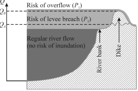
Floods occur as a result of water spilling over the crest of em-bankment (Q > QB)or more often as a result of prolong
ex-istence of high water in the embanked river channel, so when the peak flow discharge exceeds the alarm flow (QA)but is
lower than the overtopping flow (QB is the discharge that
overtops levee crests) (QAQ< Qmax< QB). One can also
distinguish many other causes of floods, such as back water and ice-jams, etc., but they do not stem from the embankment failures and will not be considered in this study.
The annual probability of inundation for embanked river reach is expressed as the total of probability of the two ex-clusive events (“Fl” stands for “flood”) (see Fig. 2):
P (Fl)=P1(Fl)+P2(Fl), (1)
where the first term comes from the conventional FFA
P1(Fl)=p(Qmax> QB). (2)
The second term of Eq. (1) defines the probability of inunda-tion caused by levees breaching which depends on both the flood persistency and levees resistance to high water stages which in turns depends on their design and technical condi-tion. Therefore, theP2(Fl) is expressed as the integral of the
[image:2.595.50.285.60.316.2]Fig. 2. Two reasons of inundation – an illustration.
the duration (d) of flow over the flow levelQA and of the
pdf of thed duration, sof (d)for annual peak flows in the intervalQA< Qmax(t ) < QB.
P2=p (Fl|(QA< Qmax≤QB) )
= ∞ Z
0+
h (Fl|d )·f (d)·dd, (3)
wheref (d)– pdf of the durationd of flows above the alarm stage; h(Fl|d) – the hazard index being the probability of levee breaching caused by a high water of the durationd.
The value of the hazard indexh(Fl|d) tends to 0 ford go-ing to 0 and to 1 ford going to infinity (e.g. Fig. 6). The hazard indexh(Fl|d)is determined administratively for the river reach by the Regional Water Management Board based on the technical assessment of flood embankments.
Note that collating the annual maximum high flow dura-tion data for analysis one putsdt =0 (indext marks thetth
year in a series in which the particular eventd=0 occurred,
t=1, 2,. . . ,T andT is the length of the series in years) the both forQmax≤QAandQmax> QB, so 1 inundation yearly
is considered and that caused by spilling over crest has the priority over that caused by prolonged high stages. Further-more, note that the weaker is the relationship between annual maximal values of peak flow and duration of flows above the alarm flow (QA)the more justified is the separate analysis of
the both random variables. The DqF approach is the exten-sion of the conventional FFA performed on a single annual peak flow series. But, even though it does not have to be the same flood that gives the annual flood peak and last longest in the year, the annual peak flows are usually assumed to be temporary independent what has been verified by several investigators and so is assumed here for the annual maxi-mal durations. Due to the poor measurement material – short samples – it would be ever harder to analyse autocorrelations in the series of durations.
The ratio of probabilitiesP2toP1and their total is
help-ful to determine the actions to reduce the risk of flooding,
namely the strengthening or heighten the levees (or building parallel levees).
3 The statistical modelling of flood hydrographs shape
Due to complexity of stochastic nature of river flow pro-cess one has to accept a rational ignorance while deal-ing with flood risk management. In response to practical needs, several simple conceptual structures are being de-veloped for statistical modelling of flood hydrographs. The methods of constructing design flood hydrographs are most popular for modelling flood hydrographs. Their reviews are available in, for example, Serinaldi and Grimaldi (2010), Strupczewski (1964, 1966) and Strupczewski et al. (2013). The design hydrographQ(t )with the defined return period of its peak serves both in flood–risk mapping procedures and for designing a reservoir storage capacity and other hy-draulic structures sensitive to flood hydrograph magnitude and shape.
The common feature of most of the approaches to flood hydrographs analysis is an avoidance of using a joint prob-ability distribution of parameters describing the shape of the hydrographs while limiting multi-dimensional analysis to conditional expectations further reduced to a regression. The most commonly used variables are flood peak and flood volume.
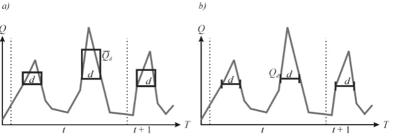
Extension of the standard FFA for statistical analysis of peak part of flood hydrographs is the one-dimensional model Flow-duration Frequency (QdF) initiated by NERC (1975) and Askhar (1980); in the 1990s, Sherwood (1994), Balocki and Burgess (1994). Gal´ea and Prudhomme (1997) laid out the foundations of the present form of the QdF method. Based on the assumption of the convergence of differ-ent flood distributions for small return periods (Javelle et al. 1999), Javelle (2001) introduced a converging approach to the QdF modelling. Here the annual mean maximum peak flood volume (or equivalently the mean excess dis-charge – Q¯d) corresponding to the given duration (d) is
taken (Fig. 3a) as the random variable. Therefore, con-sequently the maximum d−days annual outflow volume
Vd=d· ¯Qdis the random variable as well. In fact, the above
idea of flood peaks analysis is modelled on the analyses of the Intensity-duration-Frequency (IdF) commonly used for stochastic modelling of high intensity rainfalls and of the QdF analysis of low flows.
To cater to the conventional FFA, the flow discharge (QA)
corresponding to the alarm stage (HA)is used here, so the
upper limb of the rating curve is regarded as time invariant. The frequency of annual maximum uninterrupted duration of flows,D(in hours, days, etc.), over the flood alarm stage (HA)(or equivalently over the alarm flow (QA))but
exclud-ing floods pourexclud-ing over the embankment crest (which corre-sponds to flows exceeding the overtopping flowQB)serves
Fig. 3. Definition of the random variables in the QdF models: (a) the mean maximumddays flow, (b) the annual maximum flow discharge (Qd) continuously exceeded during the periodd.
channel caused by scouring the levees (Fig. 2). Therefore, thedt=0 in the [d] time series means that the threshold dis-charge,QA, has not been exceeded during thetth year of the
series (Qmax(t ) < QA)or that the peak flow has exceeded the
overtopping flow (Qmax(t ) > QB), where Qmax(t )denotes
the annual maximum discharge occurred in thetth year of the sample series. In other words, there is no risk of the dike’s damaging due to the prolonged exposure to the high water because the flood wave was either too small to reach the weaken construction of the levee or, the contrary, the flood is such big and sudden that the water immediately overtops the levee’s crest. Note that if more than one flood appears in a year, theDand the annual peak flow (Qmax)can correspond
to different floods (Fig. 1).
Using multi-duration approach, by fitting the appropri-ate statistical distribution to the extracted samples for var-ious durations, from the relations QdF for various d one can roughly construct the scaled Flood-duration-Frequency curve (QdF). To avoid inconsistency of the estimates of quan-tileQ(d,F )for variousd,the same distribution function is applied for all duration (Javelle et al., 1999; Castellarin et al., 2004; Iacobellis, 2008; Botter et al., 2008) and the quan-tiles are reduced by the appropriate functionφ (d,ν) which is decreasing function ofd:
Q (d, F )=φ (d,ν)·Q (0, F )ford=0,1,2, . . .;φ (0)=1, (4) where theνdenotes the vector of parameters which are esti-mated from the data.
It means that differences in the distributions of variousd
values result from the differences in the mean value only. Note thatQ(0,F )corresponds to the distribution of annual instantaneous peak discharges. The parameters of the func-tionφ (d,ν) andQ(0,F )(Eq. 5) are estimated separately.
Finding that flood persistence is a factor of flood hazard for embanked rivers, Bogdanowicz et al. (2008) modified the above model redefiningQas the annual maximum flow discharge (Qd)which is continuously exceeded during the
period d, wherein the d variable is still treated as a deter-ministic value (Fig. 3b). The applied way of determining the
scaled distribution function does not differ much from the method described by Javelle et al. (1999). In parallel, the use of ML method in the presence of thed as the covariate (Strupczewski et al. 2001a, b; Katz et al., 2002; Stasinopou-los and Rigby, 2007; StasinopouStasinopou-los et al., 2008, 2012) is demonstrated for Weibull distribution with the lower bound parameter and the constant shape parameter. Here all param-eters are estimated jointly.
However, to address the 1-D statistical analysis of the peak part of flood hydrographs directly to the problem of soften-ing and breachsoften-ing of river embankment, the duration (d)of high stages should be taken as a random variable rather than the mean excess discharge Q¯d (Javelle, 2001) (Fig. 3a) or
the the annual maximum flow discharge (Qd)(Fig. 3b)
(Bog-danowicz et al., 2008). Note that the duration of flood (d)can be more accurately assessed than the peak flow discharge of large floods.
4 Formal aspects of the duration–flow–frequency modelling
To address the flood risks arising from softening and washing out the river embankments, Bogdanowicz et al. (2011) pro-posed to take as the subject of analysis the frequency of an-nual maximum uninterrupted duration,D(in days), of flows over the flood alarm stage (QA), the duration (D) is
con-sidered as a random variable while the alarm flow discharge (QA)is the fixed value (Fig. 1).
The time series of annual maximum uninterrupted du-ration, D (in days), of flows over the flood alarm flow
QA, d=(d1, d2,. . . ,dt,. . . , dT), is the subject of
statisti-cal modelling in stationary and non-stationary conditions. The dt=0, denotes that the QA has not been exceeded
during the tth year (Qmax(t ) < QA) or that the peak flow
has exceeded the overtopping flow (Qmax(t )≥QB), which
[image:4.595.100.500.61.197.2]that the conditionQmax(t )≥QBis equivalent to the
uncon-ditional inundation, from Eq. (2)P1(Fl|Qmax(t )≥QB)=1,
while QB> Q(t )≥QA points to only possible inundation
(see Eq. 3).
Frequency analyses of hydrological sample with zero dis-crete values have received relatively little attention. Still there are several approaches for analysis of censored data, includ-ing probability plot, regression, weighted-moment estima-tors, maximum likelihood estimaestima-tors, and conditional prob-ability analyses (Gilliom and Helsel, 1986; Hass and Scheff, 1990; Harlow, 1989; Helsel, 1990). A consistent approach to the frequency analysis of such data requires using dis-continuous probability distribution functions. Jennings and Benson (1969), Interagency Advisory Committee on Water Data (1982), Woo and Wu (1989), Wang and Singh (1995) among others developed empirical three-parameter models for frequency analysis of hydrologic data containing zero values.
When the available data represent mean daily discharge, thed values are in fact the integer numbers (the exposition can last 1, 2, 3, etc., days) but to maintain the continuity of time we treat them as real numbers and considerdas if it cor-responded to the duration range (d– 0.5 day,d+0.5 day). In particular, ford=0 (beginning of the time axis) the interval corresponds to the range (0,d+0.5 day). If a flood starts be-fore the end of a year and is continuing to the next year, thed
value is derived for the entire flood wave (from its beginning in one year to its end in the next year) but attributed to the yeartwhen the flood culmination occurred. To get an insight into flood persistence properties, the several threshold stages (QT)are considered but not only the alarm stageQA. 4.1 Stationary conditions
As far as the probability theory is concerned, the occur-rence of zero events can be expressed by placing a non-zero probability mass on a zero value:P (D=0)6=0, where D
is the random variable, andP is the probability mass (e.g. Strupczewski et al., 2002, 2003; Weglarczyk et al., 2005). Therefore, the parent distribution functions of such hydro-logic series would be discontinuous (with discontinuity at 0) and, using the theorem of total probability, their forms can be written as
f (d)=βδ (d)+(1−β) f◦(d;g)·1(d) , (5)
where β denotes the probability of the zero event, β=
P (D=0),f◦ (d;g) is the conditional probability density function (CPDF),f◦(d;g)≡f(d|D >0), which is contin-uous in the range (0,+ ∞) with a lower bound of 0, andg is the vector of parameters (containingβor not),δ(d)is the Dirac’s delta function and 1(d)is the unit step function. As-suming the infinite upper bound forDseems acceptable and facilitates modelling. Due to discretisied durationdintervals, the probability of exceeding theQAflow during one day only
is equals to
P (d)=
d+1/2
Z
d−1/2
f (d)·dd.
Hydrological samples with zero values are most frequently of exponential-like shape. Weglarczyk et al. (2005) mod-elled CPDFf◦(d;g) of (5) by two-parameter distributions, namely by generalized pareto, Weibull and gamma, estimat-ing parameters by the maximum likelihood (ML) and the mo-ments (MOM) methods.
4.1.1 Estimation of the weight parameterβ
From the pdf of the durationd(Eq. 5) and the records
d= (d1,d2, . . . ,dt,dT) for given alarm flowQA
From Eq. (5) one can write the likelihood function as
L=βn1·(1−β)n2
n2 Y
j=1
f◦ dj;g
, (6)
wheren1andn2denote the number of zeros and non-zeros
values, respectively.
Ifβ /∈g, from ML-equations:
∂lnL
∂β =
n1
β −
n2
(1−β) =0 (7)
one can easily find that the ML-estimate ofβis ˆ
β= n1
n1+n2
(8) soβandgare estimated by MLM independently.
From CDF of annual maximum floods obtained from FFA
The better estimate of theβ parameter in the sense of def-inition (Eq. 9), not its standard error, can be obtained from the CDF of annual peaks providing the selected for Annual Maxima (AM) model fits upper tail data well. Note that the
D=0, denotes that theQAhas not been exceeded during the
tth year (Qmax(t ) < QA)or that the peak flow has exceeded
the overtopping flow (Qmax(t ) > QB)whereQmax denotes
the annual maximum discharge, therefore, probability of zero value ofD
ˆ
P (D=0)= ˆP (Qmax< QA)+ ˆP (Qmax> QB)= ˆβ (9)
should be estimated from CDF of annual peak flows got from FFA rather than from the (0, 1) time series of the d
record. Having derived from FFA the CDF of the annual peaksG (Qˆ max)≡ϕ
Qmax,hˆ
wherehˆ is the vector of pa-rameter estimates, one can get the estimate ofβas
ˆ
β= ˆG (Qmax=QA)+
1− ˆG (Qmax=QB)
Note that if more than one flood appears in a year it may hap-pen that thedt and the annual peak flowQmax(t )correspond
to different floods.
Floods in excess ofQBare unique in Polish rivers, but if
they were they should be in the FFA treated as of unknown magnitude over the theresholdQB, thus one deals with first
order right censored sample.
4.1.2 Estimation of parameters of the continuous part of Eq. (5)
ML estimate of the parameters (g) of the continuous part of PDF (Eq. 6): the conditional probability density function (CPDF).f◦ (d;g)≡f(d|D >0) off◦(d;g), can be ob-tained by solving the ML system of equations:
∂lnL
∂g =
∂
∂g
n2 X
j=1
lnf◦ dj;g
=0 forβ /∈g. (10)
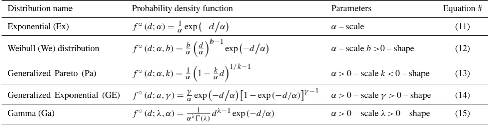
Since thedsamples deprived of the zero values are most fre-quently of exponential-like shape, the distribution functions in Table 1 are recommended as candidates for f◦ (dj; g)
model.
Note that Exponential distribution is a special case of all other mentioned above distributions, Eqs. (12)–(15).
The detailed information on the models mentioned above with the methods of ML estimation, one can easily find in hydrological and statistical literature, e.g. in Rao and Hamed (2000) and for GE in Gupta and Kundu (2000).
4.2 Non-stationary case
The non-stationary Flood Frequency Analysis has been a subject of numerous publications. Davison and Smith (1990) dealt with time-related POT approach, Strupczewski and Mitosek (1991) (later completed and published e.g. in Strupczewski and Feluch, 1997a, b, c, 1998a, b; Strupczewski et al., 2001a, b) dealt with maximum esti-mation of flood distribution functions within the presence of time as the covariate; a similar approach is presented, for example, in Katz et al. (2002) and Stasinopoulos and Rigby (2007), Stasinopoulos et al. (2008, 2012). The basic assumption in the classical Flood Frequency Analysis and the duration-flood-frequency modelling is that neither the adopted distribution function nor its parameters change in time. However, the longer the hydrological series, the harder to maintain the assumption of stationarity in the face of a changing environment and climate (Milly et al., 2008). The non-stationarity of hydrological data ought to be taken into account in FFA for theoretical and empirical reasons, but practical aspects of its introduction into design and planning procedures are not so obvious or simple and pose signifi-cant ongoing challenges to the hydrological research and wa-ter management policy. One could easily accept the increas-ing trend in design upper quantiles, but decreasincreas-ing detected trends may distort decision making in the engineering design,
evaluation of flood risk and in other flood-related issues. Es-pecially when statistical inference is based on peak flow se-ries of average length currently covering barely 60, 70 ele-ments or on climate change scenarios and their hydrological response that we presume, we are able to predict in a realis-tic manner. Herein the formal aspects of at site non-stationary Duration-Flow-Frequency modelling are presented while re-gional Flow-Duration-Frequency modelling has been intro-duced by Cunderlik and Ouarda (2006).
Assuming that only the values of parameters of the contin-uous part of the PDF may vary with time, its form remains unchanged, and the PDFf can be written as
f (d|t )=β (t ) δ (d)+[1−β (t )]f◦[d;g(t )]·1(d) . (16) Assuming the forms of trends and denoting the vectors of their parameters, respectively, asθandξ we have got
f (d|t )=β (t;θ) δ (d)+[1−β (t;θ)]f◦[d;t,ξ]·1(d);θ∈/ξ.(17) For compact notation let us define the dichotomous variable
Yt given by
Yt=
1 forD=0
0 forD >0. (18)
For the time seriesd= (d1,d2,. . . ,dt,. . . ,dT)of the maximal
annual duration of river flows exceeding the given threshold, the likelihood function can be expressed as:
L= T Y
t=1
β (t;θ)yt· T Y
t=1
(1−β (t;θ))1−yt· T Y
t=1
f◦(dt;t,ξ)1−yt (19)
and the Log-likelihood function
lnL=
T
X
t=1
yt·ln(β (t;θ))+
T
X
t=1
(1−yt)·ln(1−β (t;θ))
+
T
X
t=1
(1−yt)·ln f◦(dt;t,ξ)
. (20)
As one can see from Eq. (20), the parametersθandξ, as they are independent, can be estimated separately.
4.2.1 Estimation of parameters of the continuous part of Eq. (16) [f◦(d;t,ξ)]
The ML estimate of the parametersξ of CPDF (f◦(d;t,ξ)) are obtained by solving the system of equations:
∂lnL
∂ξ =
∂
∂ξ
T
X
t=1
(1−yt)·ln f◦(dt;t,ξ)
=0 (21)
Table 1. Distribution functions recommended asf°(dj;g) model.
Distribution name Probability density function Parameters Equation #
Exponential (Ex) f◦(d;α)= 1 αexp −d
α
α– scale (11)
Weibull (We) distribution f◦(d;α, b)= b α
d α
b−1
exp −d
α
α– scaleb >0 – shape (12)
Generalized Pareto (Pa) f◦(d;α, k)= 1 α
1−k αd
1/ k−1
α >0 – scalek <0 – shape (13)
Generalized Exponential (GE) f◦(d;a, γ )=γ αexp −d
α 1−exp(−d/α)γ−1 α >0 – scaleγ >0 – shape (14)
Gamma (Ga) f◦(d;λ, α)= 1
αλ0(λ)dλ
−1exp(−d/α) α >0 – scaleλ >0 – shape (15)
the maximum of log-likelihood function (the last component of Eq. 20) with respect to trend parameter vectorξ.
The consequence of making allowance for time-dependent parameters off◦(d;g) is an increase of the number of pa-rameters to be estimated. Given the small number of non-zero elements in the time seriesd= (d1,d2,. . . ,dt, . . . ,dT),
the number of parameters which can be effectively esti-mated is small. Therefore, we decided to adopt the values of these parameters as independent of time. Then the only non-stationarity lies in the weighting parameter β (t; θ) which plays the role of the time-dependent function “switching” on and off the event of dikes’ prolonged exposure to high waters. Note here that the durationdis a parameter that describes the shape of the flood hydrograph, so we assume that the persis-tence of flood of magnitudeQA< Qmax< QBis not subject
to time variability.
4.2.2 Two ways of estimating the time-dependent weight parameterβ(t;θ)
The estimation of parametersθof the discrete part – weight-ing parameterβ (t;θ), in the joint distribution Eq. (17), can be performed in two ways: by regression analysis and on the base of non-stationary distribution of annual maxima with time-dependent parameters.
Regression analysis
The variableYt represents binary outcomes and has a
bino-mial distribution with parameter:
β(t;θ)=P (Yt=1)=P (D=0); (22)
however, the trend inβ cannot be found by means of fre-quently assumed linear regression. The reasons of being that
– in general linear trend may take the values of probability
β(t,θ) outside the range from 0 to 1;
– the error term is not homoscedastic, nor it is normally
distributed as in normal regression.
In order to avoid values outside the range from 0 to 1 a mono-tonic transformation of the interval (0,1) is performed to the range (−∞,+∞). There are many transformations with this property, but the most popular are two: probit and logit trans-formations. Both give similar results but logit transform is more convenient for calculations. Probit transformation con-sists in converting the probability to corresponding quantiles of the standard normal distribution. Logit transformation is given by
logit=ln[β/(β−1)] (22a)
And the trend is modelled as
logit=a+bt. (22b)
Inverse transformation leads to the logistic (LO) functionβ
of timet with parameter vectorθ=[a, b].
β (t;a, b)= 1
1+exp(−(a+bt )) (23)
Logistic regression is used in many disciplines, medicine, so-cial science, econometrics, in engineering, espeso-cially for pre-dicting the probability of failure of a system or product.
Dmodel= −2 ln
likelihood of the fitted model
likelihood of the saturated model (24) and similarly, null deviance:
Dnull= −2 ln
likelihood of the null model
likelihood of the saturated model. (25) Note that in logistic regression the likelihood of the saturated model (yt=β(t;θ)) is equal 1.
The deviance has an approximate chi-square distribution with 1 degree of freedom for each predictor, so 1 in our case. Smaller values of deviance indicates better fit what corre-sponds to non-significant chi-square values.
Pseudo-R2is calculated on the base of deviances: Pseudo−R2=Dnull−Dmodel
Dnull
(26) and interpreted almost like a coefficient of determination in linear regression.
The method via annual maxima distribution with time-varying parameters
An alternative way of analyzing a trend in β is to use the non-stationary CDF of annual peaks with time-dependent pa-rameters. From NFFA (Strupczewski et al., 2001) one gets
G=ϕ(Q,h,t ), where h – the vector of PDF parameters of the annual flood peaks distribution. Then per analogy to Eq. (9a) one can write:
ˆ
β (t )= ˆP[D (t )=0]= ˆP[Qmax(t )≤QA]
+ n
ˆ
P[Qmax(t ) > QB]
o
= ˆG (QA|t )
+h1− ˆG (QB|t )
i
(27) providing the selected distribution and trend model of its pa-rameters fits the upper tail of data well. It would be advisable to compare the results of both methods. Compatibility of the results could serve as the overall test of correctness of the assumptions made.
4.2.3 Probability of inundation during the period (t1,t2)
Dealing with hydrologic design, due to non-stationarity, the notion of return period is no longer valid and the probability of inundation should refer to the whole period of life of a hydraulic structure, not to a single year as has been agreed in the stationary case.
When the parameters of DqF distribution are time depen-dent, consequently the annual probability of leves breach (Eq. 3) becomes time dependent:P2(Fl,t ). The probability
that at least once in the period (t1, t2)the inundation caused
by levees breach occurs is expressed as
P2(Fl, (t1, t2))=1−
t2 Y
t=t1
[1−P2(Fl, t )]. (28)
Similarly, if the distribution of annual maximum peaks is time dependent,G=ϕ(Q,h,t ), the exceedance probability of overflow of the levees’ crest, so the probability that (see Eq. 2)P (Qmax≥QB,t )=1−G(QB,t )=P1(Fl,t ) is time
dependent. Then the probability that the inundation caused by overtopping the embankment crest occurs at least once in the period (t1, t2)and can be expressed as
P1(Fl, (t1, t2))=p (Q > QB, (t1, t2))
=1−
t2 Y
t=t1
[1−P1(Fl, t )]. (29)
The total probability of inundation in the period (t1, t2)
equals to:
P (Fl, (t1, t2))=P1(Fl, (t1, t2))+P2(Fl, (t1, t2)). (30)
5 Example – Szczucin at Vistula River (Southern Poland)
To illustrate how the proposed approach works in practice, the Szczucin gauge (southern Poland) at the Vistula River has been selected as an example. Recent flooding in the up-per Vistula bared the weakness of the system of flood protec-tion, especially unsatisfactory condition of the embankments in the region of Szczucin. One, but not the only, major rea-son for the current state of flood protection infrastructure is a complex history of these lands. When Western European countries formed an effective flood protection scheme, Polish south-eastern lands were at the periphery of three empires, two of which were among the most undeveloped countries of the continent. After regaining independence, social and eco-nomic problems associated with merging the various districts of the reborn Poland influenced the poor development of an efficient protection system. For these reasons, embankments built during World War II do not meet current requirements which were recently put to a higher level. The Polish Peo-ple’s Republic period did not bring any important changes. Although the embankments have been periodically increased and strengthened, the high cost of post-war reconstruction and industrialization carried out under conditions of socialist economy did not allow for catching up with Western stan-dards. Lately, the material excavated on the flood land, very often at the immediate vicinity of the embankments, was used for the re-construction. As a consequence, the top layer of inactivated meadow was damaged, what facilitated the fil-tration of water from the horizontal residual layer under the layer of permeable sealer coat. There are present plans to modernise the dikes and the first works have been carried out. The investor claims that the modernisation will reduce the flooding risk by 80 %. To assess the risk before and after modernisation (provided that the statement of the investor is right) the following analysis was performed.
Fig. 4. Hydrograph of the daily flows at the Szczucin gauging
sta-tion. Horizontal dashed lines reflect theQTr values used in this
study.
have been controlled and tested with regard to the sharp dis-continuities and jumps in data – no particular irregularities have been detected (Fig. 4).
The overtopping flow QB was assessed from the rating
curve as 10 500 m3s−1which roughly corresponds to
two-hundred-years return period of annual peak flow (Q0.5 %),
the base design value for the 1st class embankments. In fact, there are no annual peak flows exceeding this value in the record. Therefore theQBvalue does not affect the
compo-sition of the vector of observation values [dt]. The alarm
threshold for the Szczucin stationQA=1690 m3s−1(which
means flow of ca. 2 yr return period, stage 660 cm); however, for completion a few other thresholds will be analysed, too, namelyQTr=700, 1000, 1300 and 2000 m3s−1. The hazard
indexh(Fl|d) forQA=1690 m3s−1(Eq. 3) was assessed as
h (Fl|d )=
0.05·d ford≤20 days
1 ford >20 days , (32)
so the embankments cannot withstand the pressure of high waters of more than 20 days.
5.1 Stationary case
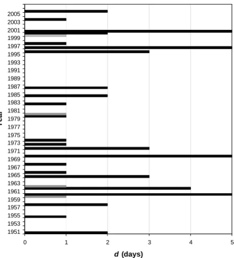
The weak correlation between the durations whend(t ) >0 (see Fig. 5) and the respective annual maximaQmax(t )
in-dicates the variety of shapes of flood hydrographs and, as a consequence,dcannot be represented (or replaced rather) in FFA byQmax. It implies the analysis of bothd andQmaxby
(perhaps) two different types of models. As a model for the parameters of thef◦function Generalised Exponential (GE) distribution has been chosen (e.g. Gupta and Kundu, 2000). Among the distributions presented in Eqs. (11)–(15), the GE distribution Eq. (14) performs relatively well in terms of the AIC value and shows stability of numerical ML solutions in
0 1 2 3 4 5
1951 1953 1955 1957 1959 1961 1963 1965 1967 1969 1971 1973 1975 1977 1979 1981 1983 1985 1987 1989 1991 1993 1995 1997 1999 2001 2003 2005
Y
e
a
r
d (days)
Fig. 5. The durations (in days) of the discharge above QA=
1690 m3s−1for Szczucin gauging station (1951–2006). The annual maximal durations are in black.
estimation of f◦ (d; g) parameters, regardless of the QTr
threshold applied for the calculations. The list of the GE es-timated parameters of the two-component DqF model andβ
values for differentQTrincludingQAis presented in Table 2.
The annual maxima are believed to be adequately de-scribed by the heavy-tailed distributions (e.g. Strupczewski et al., 2011), so to cater for the Flood Frequency Analy-sis (FFA) for extreme values (annual maxima) theβ values (Eq. 8) andP1(Fl) (Eq. 2) by means ofQmaxseries were
cal-culated with the three-parameter Generalised Extreme Value distribution:
G (q;α, γ , ε)=exp
−
h 1−γ
α(q−ε)
i1/γ
=GγGEV(x) ,(33)
From the AM sample covering the period 1951–2006 (n= 56 yr), we got the ML estimates of GEV parameters equal (for calculations we used our original soft-packages
Flood-Durations, NonstationaryMLM and SDEP which we can
eagerly share with others): location ≡ ˆε= 1260.02 m3s−1, scale ≡ ˆα = 671.39 m3s−1 and shape ≡ ˆγ=−0.33. For
completion note that the value of log-likelihood function lnL=−463.231 and thus AIC=932.461.
Substituting forq into Eq. (33), the chosenQTr andQB
values and then putting the corresponding probabilities to Eq. (9a), one gets the estimates of the weighting parameters display in Table 2.
[image:9.595.51.287.62.236.2]Table 2. The parameters of the two-component DqF model for Szczucin data.
Second component,f◦is the First component (by two methods) two-parameter Generalised Exponential
β=n1/n β=β(QTr)
QTr n2 by Eq. (9) by Eq. (9) scale shape lnML/n2
700 51 0.089 0.076 2.8799 0.2938 −2.63
1000 40 0.286 0.226 4.0392 0.5228 −2.10
1300 32 0.429 0.395 4.8616 0.7464 −1.77
1690* 23 0.589 0.577 3.4238 0.8357 −1.62
2000 17 0.696 0.683 3.7411 0.9126 −1.54
*QTr=QA.
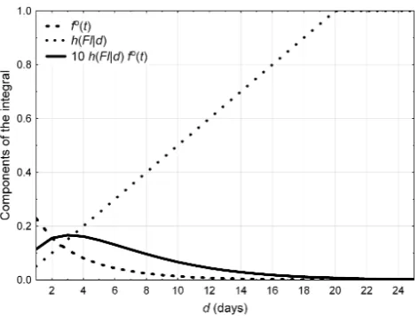
Fig. 6. Components of the integral Eq. (34).
proportionβincludes the value estimated from AM distribu-tion (Eq. 9).
Assessment of probability of levee breach along Szczucin reach
Since the event of levee breach is conditioned by the peak flow being in the range of [QA,QB], Eq. (3) can be written
as (see also Fig. 6)
P2(Fl)=(1−β)
∞ Z
0+
h (Fl|d )·f◦(d)·dd. (34)
The pdf of GE (Eq. 15) for QTr=QA= 1690 m3s−1
(Ta-ble 2) takes the form
1− ˆβ
·f◦(d;α=3.4238, γ =0.8357)
=0.423 0.2441·exp(−d/3.4238)
1−exp(−d/3.4138)0.1643
, (35)
while the ML estimate ofβequals (Table 2) 0.577. Substitut-ing them and the hazard index function defined by Eq. (32)
into Eq. (34) and integrating one gets the annual probabil-ity of levee breachingP2(Fl)=0.064. Note that at the same
time, and when the same GEV distribution is used (see the Eq. 33 and its parameters below the equation), the proba-bility of flood caused by exceeding embankment crest by annual peak flow:P1(Fl)=P (Qmax> QB=10 500 m3s−1)
=1-G(QB) is equal to 0.005, so it is almost insignificant
(more than ten times smaller than P2), hence the overall
probability of flooding along Szczucin reaches P =P1+
P2=0.069.
Variety of shapes of flood hydrographs one can evaluate by a measure of correlation strength betweenQmax(t )andd(t ).
Due to shape similarity of flood peak parts, a strong depen-dence between the peak flows (Qmax)and the duration above
the alarm flow (d)can take place. If it is the case, the proba-bilityP2(Fl) can be assessed on the base ofQmaxdistribution
g(Qmax). Assuming that d=ψ (Qmax), one can express in
Eq. (34) thedvariable by theQmaxgetting
P2(Fl)=p (Fl|(QA< Qmax≤QB) )
=
QB Z
QA
h (Fl|ψ (Qmax) )·g(Qmax)·dQmax, (36)
where per analogy to Eq. (32)h(Fl|ψ (Qmax))equals 0 and 1
forQAandQB, respectively. The Pearson’s correlation
co-efficientr(Qmax,d)for Szczucin equals to 0.83.
Of course, when estimating the risk of a levee breach, ex-cept for during the time of high water residence, more tech-nical parameters of levees should be analysed, such as the construction of the levee, the material used for its building, its age, susceptibility to softening, the regime of the river, wind-induced waving and so on. All in all, those who de-cided to build their houses in the river’s proximity behind the levees, sooner or later do experience a catastrophe.
5.2 Non-stationary case
[image:10.595.50.286.233.411.2]as components of DqF analysis show different behaviour ver-sus time. The continuous variable – duration of water level above certain stage – in general, shows no trend. It describes the shape of the flood waves which has been stated to be rather stable and, if any trend there exists, it does not pose any effect on the final results of the DqF calculations. On the other hand, a visual assessment of records for Szczucin and other hydrological stations show that the frequency of occur-rence of extreme flows (P1)and flows above (so well below)
a given threshold (QTr) may reveal some trend. Therefore
in this study we focused only on the search of trends in the probabilityP1 and in the weighting factorβ that plays the
role of the time-dependent function “switching” on and off the event of dikes’ prolonged exposure to high waters. These trends have been estimated from the annual peak flow series and by direct analysis of [dt] vector represented by the se-quence of 0 and 1 as given by Eq. (18). In both cases the maximum likelihood method (MLM) has been used for cal-culation, while the logistic function (23) serves to model the (0,1) duration series.
The estimationβ(t )for the threshold corresponding to the alarm stage (QA=1690 m3s−1) in the form of the logistic
function (26) revealed the decreasing trend (b <0), whereas
a=0.405, so theβ(t )takes the form:
βLO(t )=1+exp(0.002·t )−0.405−1 (37a) and the parameters of stationaryf◦function for selectedQTr
values can be found in Table 2.
The above equation (Eq. 37a) says that the odds (the ratio of probabilities of events against nonevents: β(t )/(1-β(t ))
decreases in average by 0.2 % from year to year, that gives the change ofβfrom ca. 0.60 in 1951 to about 0.58 in 2006. However this trend is not statistically significant. The model deviance Dmodel being equal to 75.8286 and the null
de-vianceDnull=75.8372 give the difference with p value of
0.9264 from chi-square distribution. The value of
Pseudo-R2=0.046 is close to 0. It is likely that this result points on almost stable risk of inundation caused by dike breaches for summer floods that prevail in the reach of the Vistula river represented by Szczucin hydrological station, where changes in the river bed and on the floodplains have not influenced considerably the transportation of high waters. Winter floods can reveal stronger trends due to greater variability of melt-ing condition and observed temperature rise, therefore, as consequence, the volume of runoff. Small catchments seem to be more susceptible for trends in β. These statements ought to be verified on the larger hydrological data set.
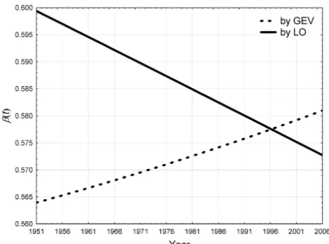
[image:11.595.309.544.61.235.2]If instead of the logistic (LO), we take the non-stationary Generalised Extreme Value (GEV) distribution function (see stationary case above), assume linear trends in mean value and standard deviation (but not in the parameters of location, scale and shape) and calculate the β(t )by means of Non-stationary Flood Frequency Analysis (e.g. Strupczewski et al., 2001, 2009), we obtain
Fig. 7. Non-stationaryβ(t )by two approaches.
βGEV(t ) (37b)
=exp
−
t·(33.067·t−22453.3)+3.812×1061.54
h
1.43·t+1.339·pt·(33.067·t−22453.3)+3.812×10⁶−275.269 i3.08
.
The comparison of the values of the non-stationary log-likelihood function and AIC, lnL= −463.078 and AIC=936.157, respectively with the stationary results re-veals that the supplement by two extra parameters to the model (those responsible for the linear trend in mean and standard deviation) worsen the estimation results. It means that for a given series size (N=56) the detected trends are in fact weak, and perhaps the addition of a few new measure-ments in series can dramatically change their value or even sign. The weakness of the trends in moments are confirmed by the weakness ofβtime variability.
The time variability of β functions obtained by the two approaches are shown in the Fig. 7.
Eqs. 37a and 37b and Fig. 7 point at the difference in trend sign ofβbetween the results received by the two approaches (LO and GEV). However, there are similarities, too. The re-sults for both cases say that the value of β is practically time independent (statistically insignificant) within time pe-riod 1951 to 2006 and thus maintain the relatively constant balance between the first and the second terms of the DqF probability density function (Eq. 17). In consequence, the durations of water stay aboveQAdescribed by thef◦
func-tion are actually as frequent nowadays as they were in past. On the other hand, the probabilityP1andP2 (and thusP )
are now the functions oft. If we take the GEV-based β(t )
as an example (as more reliable than LO-based β(t )) and
t=1 (year 1951) one obtainsP2=0.066. Further, with the
non-stationary GEV (by the same parameters as forβ(t )):
P1=0.007, so in consequence P=0.073. Fort=56 (year
2006):P1=0.004,P2=0.064, soP= 0.068, thus the
for the reader and decision makers. Please also note that re-gardless the point in time the ratioP1/P2 is similar to the
stationary conditions.
However, the probability for the certain point in time may not carry information sufficient for flood protection authority. Therefore, it is interesting to know what is the probability of inundation over the certain period, e.g. 20 yr of the exploita-tion of the dikes in Szczucin. For the GEV non-staexploita-tionary model (with the parameters mentioned above) and last 20 yr of the time series (1986–2006) the probability of overtopping over the levee crest is equal toP1=0.048, whereas the dike’s
breach probability is more than 10 times larger:P2=0.516.
Overall risk of inundation, P =0.563, is almost 10 times larger than for a single year. The reader also notes easily that again the ratioP1/P2is alike the ratios for the point-in-time
non-stationary case as well as for the stationary case. One has to bear in mind, however, that the linear trend in parameters (in case of the LO) and first two moments (as it was in GEV) is just the simplest of the countless trend pat-terns that may be employed for the time-dependent models and application of other ways (e.g. parabolic, polynomial, ex-ponential, etc.) usually leads to the overparametrization and noteworthy complication of numerical calculations. It is so, because maximum likelihood estimates for time-dependant models require multi-parameter optimisation of relatively “flat” log-likelihood functions with use of relatively short data series.
6 Conclusions
In the paper the new two-component model of flood waves, “duration of flooding-discharge-probability of non-exceedance” (DqF), with the methodology of its parame-ters estimation was proposed as a completion to the classical FFA methods. Such a model can estimate the duration (d)
of stages (and flows) exceeding the assumed magnitude with a certain probability which is of key importance when the river’s dikes are prone to the prolonged impact of high wa-ters. The embankments may be weaken by the water, soak and eventually break – this is the most frequent cause of floods in Poland. However, in this study the two main causes of inundation of embanked rivers, namely over-crest flow and wash out of the levees, were combined to assess the total risk of inundation. The proposed DqF modelling approach was generalised to the non-stationary conditions. Therefore, in addition to the maximum flow one should consider also the duration of high waters above the alarm flowQA in a river
channel. The model combined with the technical evaluation of probability of levees breach expressed by the hazard in-dex gives the annual probability of inundation caused by the embankment failure. The probability of inundation is the to-tal of probabilities of exceeding embankment crest by flood peak and the probability of washout of levees.
The DqF modelling is the consequence of QdF ap-proach developed by Javelle et al. (1999, 2000, 2002) and Bogdanowicz et al. (2008) but in the first model the gravity is put on the probability of the certain duration above alarm-ing stage/discharge (QA)rather than on magnitude of flood
itself (Qmax)like in the latter case (Fig. 3).
The DqF model in the form of Eq. (5) consists of two terms: β×δ(d) deals with the zero event,D=0, whereas the latter term (1 – β)×f◦ (d; g)×1(d) stands for the events when the durationD >0. In general bothβ andf◦
in non-stationary case may depend on time. The maximum likelihood method (MLM) was proposed for estimation of
β andg parameters. In the non-stationary case it is conve-nient to describe theβ(t;θ)by means of the logistic func-tion (23). However,β andβ(t;θ)can be also estimated by means of annual peak flows series,Qmax, using the routine
flood frequency techniques (FF) with distribution functions commonly used in FFA (e.g. GEV) for stationary and non-stationary case, respectively. Note that estimating the weight-ing factorβ andβ(t;θ)from the durationd time series the information (0,1) for excess the threshold levelQTr is used
exclusively, while based on the annual peak flow time series
Qmax, the information from whole range of recorded flood
magnitude is used to assess the trend in the alarm flowQA.
Forf◦ (dj; g) model (both stationary and non-stationary)
the exponential-like shaped distribution functions are recom-mended, such as exponential, Weibull, pareto, generalised exponential, gamma and similar.
The calculations for the Szczucin at the Vistula River case study made for several threshold values (QTr)
includ-ing the alarm flow (QA) have showed the similar results
for the weighting factor β estimated by ML method from the duration time series and from annual peaks time series (Table 2). The peak flows that could overtop the embank-ments have not been detected in the Szczucin’s record (1951– 2005). According to the hazard function (32), the possibility of levees breaching increases almost tenfold the probability of inundation.
Variability in the Szczucin time series of thed duration (understood as a time-dependence of the g parameters of
f◦ (dt; g)) has not been subject of modelling because of
accepting (sadly) the fact that the tools available are in their infancy.
The DqF model proved to be the important completion to the traditional FFA concentrating on maximal seasonal or annual discharges. The DqF approach is especially useful in polish specific conditions where the flood protection in-frastructure is dated and often does not survive confrontation with prolonged pressure of high waters.
Reliable data and information about floods are indispens-able for better understanding the interactions between rivers and flood protection system: embankments, reservoirs and polders. Improvement of statistical models is essential for en-gineering design in general and in particular for implemen-tation of flood risk mitigation procedures. Not only has the DqF modelling shown that actual flood risk is greater than the risk assessed by means of classical FFA but also vides quantitative measures which can be used in flood pro-tection systems planning, exploitation and conservation. This measures in form of dependence of inundation risk on river flow (or water level) should be established for other hydro-logical stations on Polish rivers and their dimensionless ver-sions compared. The geographic information systems tech-nique (GIS) could be used to indicate locations prone to in-undation; also, the GIS can be a helpful tool to visualisation and testing trends in the structure of river network and to the regional analysis. These results can constitute the theoreti-cal background to a number of practitheoreti-cal decisions in water management issues.
Acknowledgements. The authors would like to thank Janusz ˙
Zelazi´nski for inspiring discussions and exchange of ideas, with-out which this work would not have its present form and meaning. Sincere thanks for a sense of realism and keeping both feet on the ground what in face of many sources of uncertainty, so typical for hydrology, helped us to work out practical solution to the problem.
This research project was partly financed by the grant of the Polish National Science Centre titled “Modern statistical models for analysis of flood frequency and features of flood waves”, decision nr DEC- 2012/05/B/ST10/00482, the Grant Iuventus Plus IP 2010 024570 “Analysis of the efficiency of estimation methods in flood frequency modelling” and made as the Polish contribution to COST Action ES0901 “European Procedures for Flood Frequency Estimation (FloodFreq)”.
Edited by: E. Gargouri-Ellouze
References
Askhar, F.: Partial duration series models for flood analysis, PhD Thesis, Ecole Polytechnique de Montr´eal, Montr´eal, Canada, 1980.
Balocki, J. B. and Burges, S. J.: Relationships between n-day flood volumes for infrequent large floods, J. Water Resour. Plann. Man-age., 120, 794–818, 1994.
Bogdanowicz, E., Strupczewski, W. G., and Kochanek, K.: Appli-cation of Discharge-duration-Frequency model for description of peak part of flood hydrograph, Przeglad Geofizyczny, LIII, 3-4, 263–288, 2008 (in Polish).
Bogdanowicz, E., Strupczewski, W. G., and Kochanek, K.: Per-sistence as a factor of flood hazard for embanked rivers. EGU Leonardo Conference “Floods in 3D”, Bratislava 23–25 Novem-ber, Abstract in Proceedings, 2011.
Botter, G., Zanardo, S., Porporato, A., Rodriguez-Iturbe, I., and Rinaldo, A.: Ecohydrological model of flow duration curves and annual minima, Water Resour. Res., 44, W08418, doi:10.1029/2008WR006814, 2008.
Castellarin, A., Vogel, R. M., and Brath, A.: A stochastic index flow model of flow duration curves, Water Resour. Res., 40, W03104, doi:10.1029/2003WR002524, 2004.
Cunderlik, J. M. and Ouarda, T. B. M. J.: Regional flood-duration-frequency modelling in changing environment, J. Hydrol., 318, 276–291, 2006.
Davison, A. C. and Smith, R. L.: Models for exceedances over high thresholds, J. Roy. Stat. Soc. B, 52, 393–442, 1990.
Eagleson, P. S.: Dynamics of flood frequency, Water Resour. Res., 8, 878–898, 1972.
Gal´ea, G. and Prudhomme, C.: Notations de bases et concepts utiles pour la comprehension de la mod´elisation synth´etique des r´egimes de crue des basins versants au sens des modeles QdF, Rev. Sci. Eu., 1, 83–101, 1997.
Gilliom, R. J. and Helsel, D. R.: Estimation of distributed param-eters for censored trace level water quality data-1. Estimation techniques, Water Resour. Res., 22, 1201–1206, 1986.
Gioia, A., Iacobellis, V., Manfreda, S., and Fiorentino, M.: Runoff thresholds in derived flood frequency distributions, Hydrol. Earth Syst. Sci., 12, 1295–1307, doi:10.5194/hess-12-1295-2008, 2008.
Gupta, R. D. and Kundu, D.: Generalized Exponential Distribu-tion: Different Method of Estimations, J. Statist. Comput. Simul., 2000, Vol. 00, pp. 1 – 22, 2000.
Haas, C. N. and Scheff, P. A.: Estimation of averages in truncated samples, Environ. Sci. Technol., 24, 912–919, 1990.
Harlow, D. G.: Effect of proof-testing on the Weibull distribution, J. Material Sci., 24, 1467–1473, 1989.
Helsel, D. R.: Less than obvious: statistical treatment of data below detection limit, Environ. Sci. Technol., 24, 1767–1774, 1990. Iacobellis, V.: Probabilistic model for the estimation of T year
flow duration curves, Water Resour. Res., 44, W02413, doi:10.1029/2006WR005400, 2008.
Iacobellis, V., Gioia, A., Manfreda, S., Fiorentino, M.: Flood quan-tiles estimation based on theoretically derived distributions: re-gional analysis in Southern Italy. Nat. Hazards Earth Syst. Sci., 11, 673–695, doi:10.5194/nhess-11-673-2011, 2011.
Interagency Advisory Committee on Water Data: Guidelines for de-termining flood flow frequency. Bulletin 17B, US Department of the Interior, Geological Survey, Office of Water Data, Reston, Va, 1982.
Javelle, P., Gr´esillon, J. M., and Gal´ea, G.: Discharge-duration-frequency curves modelling for floods and scale invariance. Comptes Rendus de l’Academie des Sciences, Sciences de la terre et des planets, 329, 39–44, 1999.
Javelle, P., Gal´ea, G., and Gr´esillon, J. M.: L’approche debit-dur´ee-fr´equ´ence: historique et avanc´ees, Revue des Sciences de la terre et des plan´etes, 329, 39–44, 2000.
Javelle, P., Ouarda, T. B. M. J., Lang, M., Bob´ee, B., Gal´ea, G., and Gr´esillon, J. M.: Development of regional flood-duration-frequency curves based on the index-flood method, J. Hydrol., 258, 249–259, 2002.
Jennings, M. E. and Benson M. A.: Frequency curve for annual flood series with zero events or incomplete data, Water Resour. Res., 51, 276–280, 1969.
Kaczmarek, Z.: Statistical Methods in Hydrology and Meteorol-ogy, Sec. 4.5, 205–217, Published for the Geological Survey, US Department of the Interior and the National Science Founda-tion, Washington, DC (translation of Polish book, 1970), 320 pp., 1977.
Katz, R. W., Parlange, M. B., and Naveau, P.: Statistics of extremes in hydrology, Adv. Water Resour., 25, 1287–1304, 2002. Milly, P. C. D., Betancourt, J., Falkenmark, M., Hirsch, R. M.,
Kundzewicz, Z. W., Lettenmaier, D. P., and Stouffer, R. J.: Sta-tionarity Is Dead: Whither Water Management?, Science, 319, 573–574, doi:10.1126/science.1151915, 2008.
NERC: Flood Studies Report. Estimation of flood volumes over dif-ferent durations, 1–2, 243–264, Ch. 3, Nat. Environ. Res. Coun-cil, London, Vols. 1–5, 1100–pp., 1975.
Rao, A. R. and Hamed, K. H.: Flood frequency analysis, CRC Press, 2000.
Serinaldi, F. and Grinaldi, S.: Synthetic Design Hydrographs Based on Distribution Functions with Finite Support, J. Hydrol. Eng. ASCE, 16, 435–446, 2010.
Sherwood, J. M.: Estimation of volume-duration-frequency rela-tions of ungauged small urban streams in Ohio, Water Resourc. Bullet., 30, 261–269, 1994.
Sivapalan, M., Wood, E. F., and Beven, K. J.: On hydrologic sim-ilarity, 3, A dimensionless flood frequency model using a gen-eralized geomorphologic unit hydrograph and partial area runoff generation, Water Resour. Res., 26, 43–58, 1990.
Stasinopoulos, D. M. and Rigby, R. A.: Generalized additive models for location scale and shape (GAMLSS) in: R. J. Stat. Softw., 23, 1–46, 2007.
Stasinopoulos, M., Rigby, B., and Akantziliotou, C.: Introductions on How to Use the GAMLSS Package in R (2nd Edn.), 11 Jan-uary, 2008.
Stasinopoulos, M., Rigby, B., and Akantziliotou, C.: Instructions on how to use the GAMLSS package in R. Second Edition, Febru-ary 25, See Ch. 6., Model selection. 6.2., Selecting Explanatory variables using addterm, dropterm and step AIC, 2012. Strupczewski, W.: Flood hydrograph equation, Bulletin du
Ser-vice Hydrologique et Meteorologique, Wyd. Komunikacji i Lacznosci, Fascicule 57, 2/1964, 35–58, 1964 (in Polish: R´ownanie fali powodziowej).
Strupczewski, W.: Statistical analysis of shapes of flood hydro-graphs, Doctoral Dissertation, Warsaw Technical University, p. 181 plus Tables 25 and Figures 39, (in Polish: Statystyczna analiza kształt´ow fal wezbraniowych), 1966.
Strupczewski, W. G. and Feluch, W.: System of identification of an optimum flood frequency model with time dependent parameters (IDT). in: Integrated Approach to Environmental Data Manage-ment Systems, edited by: Harmancio˘glu, N., Kluwer Acad. Publ., 291–300, 1997a.
Strupczewski, W. G. and Feluch, W.: Floods study of the Polish rivers by the IDT soft tool, Annales Geophysicae, Part II, Hydrol-ogy, Oceans, Atmosphere & Nonlinear Geophysics, Supplement II to Volume 15, C-310, 1997b.
Strupczewski, W. G. and Feluch, W.: System of identification of an optimum flood frequency model with time dependent parame-ters (IDT), in: Integrated Approach to Environmental Data man-agement Systems, edited by: Harmancio˘glu, N., Kluwer Aca-demic Publishers, 291–300, Presented at NATO-ARW “Inte-grated Approach to Environmental Data Management Systems” Izmir, September, 1997c.
Strupczewski, W. G. and Feluch, W.: Flood frequency analysis un-der non-stationarity, Geographia Polonica, 71, 19–34, 1998a. Strupczewski, W. G. and Feluch, W.: Investigation of trend in
an-nual peak flow series. Part. I. Maximum likelihood estimation, Proceedings of the Second International Conference on Climate and Water V.1, 241–250, 1998b.
Strupczewski, W. G. and Kaczmarek Z.: Non-stationary approach to at-site flood-frequency modelling. Part II. Weighted least squares estimation, J. Hydrol., 248, 143–151, 2001.
Strupczewski, W. G. and Mitosek, H. T.: How to deal with non-stationary time series in the hydrologic projects, Mitteilungs-blatt des Hydrographishen Dienstes in Osterreich, Nr.65/66,36-40, Presented at IAHS Symposium, Vienna, 1991.
Strupczewski, W. G., Singh, V. P., and Feluch, W.: Non-stationary approach to at-site flood-frequency modelling. Part I. Maximum likelihood estimation, J. Hydrol., 248, 123–142, 2001a. Strupczewski, W. G., Singh, V. P., and Mitosek, H. T.:
Non-stationary approach to at-site flood-frequency modelling. Part III. Flood analysis of Polish rivers, J. Hydrol., 248, 152–167, 2001b. Strupczewski, W. G., Singh, V. P., and Weglarczyk, S.: Physi-cally based model of discontinuous distribution for hydrolog-ical samples with zero values, Proceedings of the Int. Conf. On WaRMAR, Kuwait, Surface Water Hydrology, edited by: Singh, Al-Rashed and Sherif, A.A. Balkema Publishers, Swets & Zeitlinger, Lisse, 523–537, 2002.
Strupczewski, W. G., Weglarczyk, S., and Singh, V. P.: Impulse re-sponse of the kinematic diffussion model as a probability distri-bution of hydrologic samples with zero values, J.Hydrol., 270, 328–351, 2003.
Strupczewski, W. G., Kochanek, K., Feluch, W., Bogdanowicz, E., and Singh, V. P.: On seasonal approach to non-stationary flood frequency analysis, Phys. Chem. Earth, 34 pp., 612–618, 2009. Strupczewski, W. G., Kochanek, K., Markiewicz, I.,
Bogdanow-icz, E., Weglarczyk, S., and Singh V. P.: On the tails of dis-tributions of annual peak flow, Hydrol. Res., 42, 171–192, doi:10.2166/nh.2011.062, 2011.
Wang, S. X. and Singh, V.,P.: Frequency estimation for hydrologi-cal samples with zero values, J. Water Resour. Plann. Manage., ASCE, 121, 98–108, 1995.
Woo, M. K. and Wu, K.: Fitting annual floods with zero flows, Can. Water Resour. J., 14, 10–16, 1989.