Soil moisture controls on patterns of grass green up in Inner Mongolia: an index based approach

(1)

Hydrol. Earth Syst. Sci., 17, 805–815, 2013 www.hydrol-earth-syst-sci.net/17/805/2013/ doi:10.5194/hess-17-805-2013

EGU Journal Logos (RGB)

Advances in

Geosciences

Open Access

Natural Hazards

and Earth System

Sciences

Open Access

Annales

Geophysicae

Open Access

Nonlinear Processes

in Geophysics

Open Access

Atmospheric

Chemistry

and Physics

Open Access

Atmospheric

Chemistry

and Physics

Open Access Discussions

Atmospheric

Measurement

Techniques

Open Access

Atmospheric

Measurement

Techniques

Biogeosciences

Open Access Open Access

Biogeosciences

Discussions

Climate

of the Past

Climate

of the Past

Discussions

Earth System

Dynamics

Earth System

Dynamics

Discussions

Geoscientific

Instrumentation

Methods and

Data Systems

Open Access

_{Geoscientific}

Instrumentation

Methods and

Data Systems

Geoscientific

Model Development

Geoscientific

Model Development

Discussions

Hydrology and

Earth System

Sciences

Open Access

Hydrology and

Earth System

Sciences

Ocean Science

Discussions

Solid Earth

Discussions

The Cryosphere

Discussions

Natural Hazards

and Earth System

Sciences

Open Access

Discussions

Soil moisture controls on patterns of grass green-up

in Inner Mongolia: an index based approach

H. Liu1, F. Tian1, H. C. Hu1, H. P. Hu1, and M. Sivapalan2

1_{State Key Laboratory of Hydroscience and Engineering & Department of Hydraulic Engineering, Tsinghua University,}

Beijing, 100084, China

2_{Department of Civil and Environmental Engineering, University of Illinois at Urbana Champaign, Urbana, IL 61801, USA} Correspondence to: F. Tian ([email protected])

Received: 5 October 2012 – Published in Hydrol. Earth Syst. Sci. Discuss.: 12 October 2012 Revised: 1 February 2013 – Accepted: 4 February 2013 – Published: 26 February 2013

Abstract. Water availability is one of the most important environmental controls on vegetation phenology, especially in semi-arid regions. It is often represented in terms of soil moisture in small-scale studies, whereas it tends to be rep-resented by precipitation in large-scale (e.g., regional) stud-ies. Clearly, soil moisture is the more appropriate indica-tor for root water uptake and vegetation growth/phenology. Its potential advantage and applicability needs to be demon-strated at regional scales. The paper presents a data-based regional study of the effectiveness of novel water and temperature-based indices to predict spring vegetation green-up dates based on the Normalized Difference Vegetation In-dex (NDVI) observations in the grasslands of Inner Mongo-lia, China. The macro-scale hydrological model, VIC (Vari-able Infiltration Capacity), is employed to generate a soil moisture database across the region. In addition to a stan-dard index based on temperature, two potential hydrology-based indices for prediction of spring onset dates are defined, based on the simulated soil moisture data as well as on ob-served precipitation data. Results indicate that the correspon-dence between the NDVI-derived green-up onset date and the soil-moisture-derived potential onset date exhibits a sig-nificantly better correlation as a function of increasing arid-ity compared to that based on precipitation. In this way the soil-moisture-based index is demonstrated to be superior to the precipitation-based index in terms of capturing grassland spring phenology. The results also showed that both of the hydrological (water-based) indices were superior to the ther-mal (temperature-based) index in determining the patterns of grass green-up in the Inner Mongolia region, indicating wa-ter availability to be the dominant control on average. The

understanding about the relative controls on grassland phe-nology and the effectiveness of alternative indices to capture these controls are important for future studies of vegetation phenology change under climate change.

1 Introduction

(2)

directly from flow observations. Thompson et al. (2011) and Ye et al. (2012) showed that not accounting for vegetation phenology can lead to poor predictions of both seasonal evaporation and runoff variability in the northeastern USA, and that a temperature correction that mimics the phenology can help to improve the predictions. More globally, Cayan et al. (2001) showed that in areas of the world with significant deciduous forests, changes in transpiration associated with phenology can contribute to significant changes in seasonal runoff.

Vegetation phenology is influenced by variations in sev-eral environmental factors such as temperature, water avail-ability, solar irradiance, and atmospheric oxygen (Lambers et al., 2008), among which water and temperature (collectively called hydrothermal conditions) are the most important ones and are frequently chosen as variables in phenological stud-ies. Studies show that timings of most phenological events in the temperate ecosystems are significantly related to temper-ature, which means that such events are likely to occur earlier as the climate warms (Sparks et al., 2000). But in semi-arid and arid regions, spring green-up may be limited by either water or temperature availability, and the condition that lim-its green-up in any specific year may switch between the two. The water condition is likely to limit green-up in dry or warm years, while the thermal condition is likely to limit green-up in cooler or wetter years.

Numerous research efforts have been devoted to quantify-ing the relationships between phenophases and the control-ling or limiting environmental factors. One classic example is the degree day concept, which is defined as the daily ac-cumulation of air temperature above a certain (base) thresh-old value during a specific pseasonal period (see the re-view by Wang, 1960). This concept attempts to capture the thermal condition needed to be satisfied for vegetation phe-nological development. It was later extended to include the stress degree day concept to include water stress effects (Idso et al., 1978). Considerable work has been conducted in dif-ferent geographical and climatic regions to understand and quantify the relationships among climate, soil moisture, and phenology for various types of vegetation, such as tomatoes (Weaver et al., 1988), woody vegetation cover (Seghieri et al., 2009), semi-deciduous (Do et al., 2005), and drought de-ciduous (Jolly and Running, 2004) vegetation types. Most of these studies have been primarily based on ground measure-ment of phenological features and environmeasure-mental variables.

Such ground measurements cannot be easily extrapolated to characterize large-scale regional vegetation phenology, such as regional patterns and broad-scale changes in time. Remote sensing imagery has been widely used over the past two decades for monitoring vegetation dynamics at regional to global scales in view of its synoptic coverage and repeated temporal sampling (Reed et al., 1994; Zhang et al., 2003; Julien and Sobrino, 2009; Yang et al., 2012; among many others). This approach also facilitates other kinds of stud-ies that seek to explore the driving factors behind phenology

change in the context of climate change (Piao et al., 2006; Wang et al., 2011; Shen et al., 2011). In these studies, hy-drothermal conditions are almost always represented by the degree day concept applied to air temperature (for thermal condition) and precipitation (for water condition). Although soil moisture is a more direct and straightforward index that governs vegetation growth and is frequently used in lo-cal studies involving ground measurements, precipitation re-places it in remote sensing-based studies.

Recent advances in hydrological modeling capability, es-pecially at large-catchment or regional scales now provide a sound basis for estimating or predicting large-scale soil mois-ture with which to analyze and interpret observed space–time patterns in vegetation phenology. A suite of macro-scale hy-drological models has been developed that can incorporate sufficient physics to account for the water and energy bal-ances across the land surface. These models can run at spatial and temporal scales much finer than those of climate models and observed meteorological data. The macro-scale hydro-logical models can already perform reliable simulations of real-time soil moisture and streamflow at daily or sub-daily time steps. Inspired by these recent advances in modeling ca-pability, one of the goals of this research is to demonstrate the advantage of model-produced soil moisture over observed precipitation for analyzing vegetation phenological change.

In this paper we focus on grass phenology. In the case of grasslands, the phenophases include green-up in spring, ma-turity in summer, senescence in autumn and hibernation in winter. Green-up is the date of onset of photosynthetic ac-tivity, the first phenological event, which plays an important role in the whole life cycle of grasses, and can influence the biomass productivity, biodiversity evolution, water balance and carbon balance at local, regional and global scales. Here we focus on the spring grass green-up onset, which is likely to be affected by variations in thermal and moisture supply. The aim is to investigate the soil moisture and temperature controls on grass green-up onset, including the feasibility of using a soil-moisture-based index for its analysis and its ad-vantages over a precipitation-based index. The Inner Mon-golia grassland area (IMGA) is selected as the study area. The Advanced Very High Resolution Radiometer (AVHRR) Normalized Difference Vegetation Index (NDVI) data pro-vided by the Global Inventory Monitoring and Modeling Studies (GIMMS) are used to characterize grass phenology. The distributed Variable Infiltration Capacity (VIC) hydro-logical model is applied over the IMGA region to generate the distributed soil moisture data used to construct the soil-moisture-based index.

(3)

results and additional results that bring out the spatial pat-terns and temporal trends in the timing of grass green-up in the study area under an apparent warming trend found in the region. We also use the results of the analysis to demon-strate the superiority of the soil-moisture-based index over the precipitation-based index, and together with these investi-gate if and how the dominant factors that control grass green-up vary in space regionally and in time. This is followed by a brief summary and conclusions in Sect. 4.

2 Methodology

2.1 Study area and data

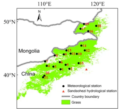
[image:3.595.323.528.61.249.2]

The IMGA is located in northern China (Fig. 1). The area has an average altitude of 1100 m a.s.l. (above sea level) and an area of 3.1×105km2. The meteorological data are from the China Meteorological Data Service System (http: //cdc.cma.gov.cn/). The study area has 21 stations (see Fig. 1) with records from 1982 to 2006. The mean annual temper-ature ranges from −3 to 7◦C, which increases from north to south. Annual precipitation ranges from 100 to 400 mm, with a mean value of 300 mm, and principally falls be-tween May and September. The mean annual pan evapora-tion (E20) is 2030 mm. The climate is dry (arid), and the study area belongs to the inland region of China. The dom-inant vegetation type in the IMGA is grass, as shown in Fig. 1, which is classified according to the MODIS product MOD12C1. The AVHRR NDVI time series data of GIMMS (http://glcf.umiacs.umd.edu/data/gimms/) from 1982 to 2006 are used to capture the timing of grass spring green-up on-set. The Sandaohezi hydrological station on Luan River (see Fig. 1) close to the study area is chosen to assess the predic-tions of the VIC hydrological model.

2.2 Macro-scale hydrologic model

The VIC model (Liang et al., 1994) was used in this study to simulate the space–time dynamics of soil moisture across the region. VIC is a physically based, semi-distributed macro-scale hydrological model that balances both water and sur-face energy within a grid cell. The VIC model can account for sub-grid variability of land surface vegetation classes and soil moisture storage capacity, and includes an infiltration al-gorithm that accounts for the areal extent of soil saturation. Soil layer depths, infiltration, and baseflow parameters have to be calibrated. VIC has been widely used for streamflow simulation and drought monitoring in large river basins glob-ally, and across China (e.g., Yuan et al., 2004; Sheffield and Wood, 2007). In this study the VIC model was implemented across China at a 0.5◦ resolution from 1951 to 2010. The model parameters were calibrated using the method proposed by Xie et al. (2007).

25

1

Fig. 1. Study area and gauging stations.

2 Fig. 1. Study area and gauging stations.

2.3 Green-up onset date and the Holdridge aridity index

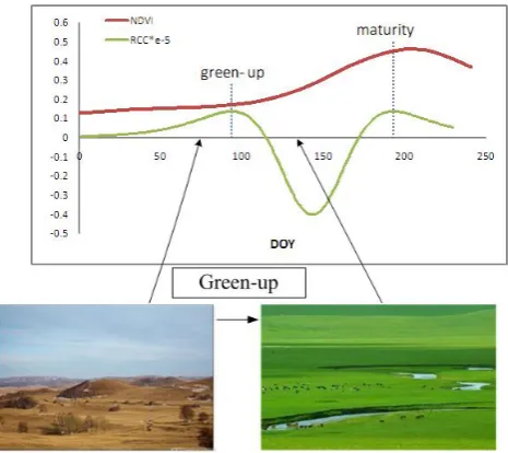
Zhang et al. (2003) defined the green-up onset date (GUD) as the day when the rate of change of the NDVI curvature (RCC) reaches its first local maximum value (see Fig. 2). We adopted this method to capture the grass GUD from the satellite images. The NDVI data marked as having good val-ues were averaged within a 3×3 pixel window. A Savitzky– Golay filtering procedure was applied to each annual time se-ries of NDVI to obtain a smoothed sese-ries (Chen et al., 2004; Shen et al., 2011). Afterwards, the smoothed series was fitted by the following four-parameter logistic function (Zhang et al., 2003; Shen et al., 2011):

NDVI(t )=c/1+ea+bt+d, (1) where the symbolsa,b,candd are best-fit model param-eters, withd being the initial background NDVI value, and

c+dbeing the maximum NDVI value. An expression for the rate of change of curvature (RCC) was derived from Eq. (1) as follows:

RCC=b3c z×3z(1−z) (1+z)3h2(1+z)3+b2c2zi

h

(1+z)4+(b c z)2i2.5−b3c z×(1+z)2

1+2z−5z2

h

(1+z)4+(b c z )2i1.5, (2) wherez=ea+bt.

[image:3.595.306.548.556.637.2]

(4)

[image:4.595.51.284.62.269.2]

26 1

Fig. 2. Rate of change of curvature (RCC) of fitted NDVI series by a four-parameter logistic 2

function (the two pictures are not exactly taken at the same place, but both are in Inner 3

Mongolia). 4

Fig. 2. RCC of fitted NDVI series by a four-parameter logistic func-tion (the two pictures are not exactly taken at the same place, but both are in Inner Mongolia).

aridity of the stations with the Holdridge aridity index (HAI) (Holdridge, 1947). The HAI index is defined as follows:

HAI=58.93×XT /365×P , (3)

where P is the annual precipitation (mm); T is the daily mean temperature within the range of 0 to 30◦C, which is excluded from the calculation whenT is less than the lower limit and assigned a value of 30◦C whenT is greater than the upper limit.

2.4 Proposed environmental indices

The factors influencing vegetation green-up include irradi-ance, temperature, soil moisture etc., amongst which the thermal and water conditions have been of most concern to large-scale vegetation phenology researchers (Yu et al., 2003; Jolly and Running, 2004). However, the relationship between green-up onset and the controlling factors can be complex, and the limiting environmental factor may shift (between places and between years) according to the pre-vailing hydrothermal conditions. Taking the example of wa-ter availability, depending on their biophysical characwa-teristics and physiological features of the vegetation, one can expect that dormant vegetation will not green-up immediately upon seeing the first rainfall – a behavior characteristic that can be explained by way of self-protection to avoid water deficit in the subsequent growth stage, in case the rainfall does not persist. This means that water accumulation through precip-itation must reach a threshold over some time span before vegetation would green up (Zhang and Liang, 2007). These notions of accumulation, threshold and time span apply to other environmental factors as well, such as temperature.

In the past, to explore the relationships between the envi-ronmental factors and vegetation green-up, it has been com-mon to accumulate the indicator variables over a fixed time span (Yu et al., 2003), for example the (typical spring) month of May. However, this has the drawback that it is quite pos-sible that vegetation green-up may have already occurred by the middle of May. Accumulation over the whole month of May complicates the relationship and contributes to poor pre-dictability. Recently, a more flexible and appropriate time span was developed by Shen et al. (2011) for the concept of thermal spring onset date (TSO). The TSO was defined as the date when the green-up can potentially begin, which means the daily temperature accumulated from a certain day to the TSO is above a threshold required for vegetation green-up. Similarly (and in addition) to the definition of TSO, we propose and compare two alternative indices that account for the control of water availability on the potential GUD, i.e., the date by which the water requirement for the onset of green-up is satisfied. First, we define the soil moisture spring green-up onset date (SMSO) as the date by which the ac-cumulated soil moisture storage reaches a threshold that the grass needs to green-up. Secondly, we also adopt an alterna-tive precipitation-based index, the precipitation spring green-up onset date (PSO), defined as the date by which the ac-cumulated precipitation reaches a depth threshold that grass needs to green up. In each case (temperature, soil moisture, precipitation), there are three components to the definition of the indices: (1) the end day of the accumulation period; (2) the time span; (3) the threshold. In this study we use the GUD detected from the remote sensing data as the end day of the accumulation period. For any chosen time span, we use the mean of the 25-yr accumulation over that time span as the corresponding threshold value. We then optimize the magnitude of the time span through the use of a maximiza-tion procedure proposed by Shen et al. (2011). Details of the optimization procedure are described below.

2.4.1 Accumulation threshold

If the time span chosen is Ndays, the corresponding

accu-mulation threshold is defined as the 25-yr (1982 to 2006) average of theNdays-accumulated soil moisture (termed as

ASMN):

ASMN =1/25

2006

X

year=1982





GUDyear−1 X

i=GUDyear−N SMi_year



, (4)

where SMi_yearis the soil moisture for thei-th DOY in a spe-cific year.

GivenNdays and ASMN, we then define the SMSO of a certain year (i.e., denoted SMSON₁₉₈₂days for the year 1982) as the last day of anNdays window that fulfills the following

(5)

moving window starting from the first day of 1982 until the accumulated soil moisture reaches ASM5, upon which we

record the last day of the current window as SMSO5₁₉₈₂. 2.4.2 Variable time span

After estimating the SMSO for each year between 1982 and 2006, we have an annual time series of SMSO value for a givenNdays:

SMSONdays ₌ n

SMSON₁₉₈₂days,SMSON₁₉₈₃days, ..., SMSON₂₀₀₆days o

. (5) We can repeat this procedure for several values of Ndays,

and in this way obtain several time series of SMSO val-ues. We assume that the potential GUD accounting for water availability should be positively cross-correlated to the GUD time series detected from the remote sensing data. Guided by this thinking, the time span of accumulation (the number of days,Ndays, preceding the known GUD) was then determined

as the value ofNdays (Note: 1≤Ndays≤90 in steps of one

day) that produces the maximum cross-correlation coeffi-cient between the annual time series of SMSONdays_{and GUD.} The maximization algorithm can be formally presented as follows:

Maximize: cross-correlation GU D, SMSONdays ₍₆₎ GU D= {GUD1982, GUD1983, ...,GUD2006}. (7)

The GUD included in Eqs. (6) and (7) is a vector consisting of annual GUD values from 1982 to 2006.

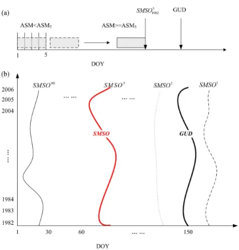
Figure 3b presents the maximizing procedure in a schematic form, where the black bold line represents the GUD series from 1982 to 2006, and the other lines stand for SMSONdays _{with different} _N

days. After comparing the

correlation between GU D and SMSONdays_{, we could get} the largest correlation coefficient and the corresponding SMSONdays_{. In Fig. 3b the optimal accumulation time span} is 5 days, which is labelled asSMSO5and shown as a red bold line, and the corresponding accumulation threshold is labeled as ASM5.

Following this maximization process, the SMSO, ASMN_SM, and corresponding optimal value ofNdays(denoted

as NSM), and the resulting optimal cross-correlation

coef-ficient between the GUD and SMSO time series are deter-mined for each measurement station. The same procedure is also followed for the case of precipitation and temper-ature, and correspondingly we obtain the values of P SO, APNP,NP, and the optimal cross-correlation coefficient be-tween GUD and PSO time series, and likewise for the values ofT SO, ATNT,NT, and the optimal cross-correlation coeffi-cient between GUD and TSO time series. These will be used later for a comparative assessment of the three indices.

27 1

Fig. 3. (a) Schematic chart of the definition of Soil Moisture Spring Onset date 2

(SMSO), a fixed window (e.g., 5-day) moving afterward from the first day of the year 3

(e.g., 1982) until the accumulated soil moisture reach the threshold ASM5, then the 4

last day of the window is 5 1982

SMSO ; (b) The maximizing process to get the optimal 5

length of accumulation period. For each window (e.g., 1 to 90), we get the 6

corresponding time series of SMSO from 1982 to 2006 (i.e., SMSO1, ..., SMSO90), 7

after calculating the correlation between each SMSO time series with GUD time 8

series, we could pick out the SMSO time series with the best correlation coefficient, 9

then the corresponding window size is the optimal length of accumulation period (i.e., 10

5). 11

Fig. 3. (a) Schematic chart of the definition of SMSO, a fixed win-dow (e.g., 5-day) moving afterward from the first day of the year (e.g., 1982) until the accumulated soil moisture reaches the thresh-old ASM5, then the last day of the window is SMSO5₁₉₈₂. (b) The

maximizing process to get the optimal length of accumulation pe-riod. For each window (e.g., 1 to 90), we get the corresponding time series of SMSO from 1982 to 2006 (i.e., SMSO1, ..., SMSO90), af-ter calculating the correlation between each SMSO time series with GUD time series, we could pick out the SMSO time series with the best correlation coefficient, then the corresponding window size is the optimal length of accumulation period (i.e., 5).

2.5 Regression of GUD based on a dominant thermal/hydrological index

The estimation procedure described above for the three envi-ronmental indices considered water and temperature as alter-native controls. In reality their effects on the GUD must be considered together, not in isolation (i.e., one or the other). If they are to be considered together and regressed together against estimated GUD values, then the question arises as to what accumulation time span to use. We address this prob-lem in this study by alternatively choosing water or temper-ature as the dominant control, and the remaining one (as the case may be) as a secondary control. In each case the chosen time span is that of the dominant control. For example, if soil moisture is assumed as the dominant control, then both soil moisture and air temperature are accumulated overNSMdays

ahead of the GUD each year, as defined below:

SMNSM

year =

GUD−NSM X

i=GUD−1

[image:5.595.309.546.57.304.2]

(6)

28

[image:6.595.66.268.61.250.2]

1

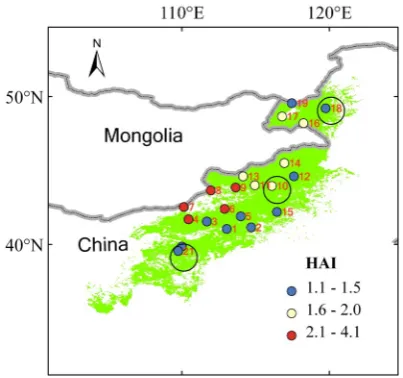
Fig. 4. The Holdridge Aridity Index of meteorological stations in Inner Mongolia grassland.

2 Fig. 4. The Holdridge aridity index of meteorological stations in

Inner Mongolia grassland area.

TNSM

year =

GUD−NSM X

i=GUD−1

T_yeari , (9)

where the year is{1982, 1983, ..., 2006}. In this way we obtain the following vectors and regress the GUD values on both SMNSM _and_TNSM _{simultaneously through multiple} regression:

SMNSM ₌n_SMNSM

1982, SM

NSM

1983, ...,SM

NSM

2006

o

(10) TNSM ₌n_TNSM

1982, T

NSM

1983, ..., T

NSM

2006

o

(11) GU DSM_reg =β1SMNSM+β2TNSM +β3 (12)

r_SMGUD=correlGU D,GU DSM_reg, (13) where β1, β2, and β3 are the regression coefficients, and

r_SMGUDis the correlation between NDVI-derived GUD and the regressed GUD (GU DSM_reg). Note that both soil moisture and precipitation are used as alternative controls to represent wa-ter availability. Using a similar procedure (as above),PNP_, TNP_{, and}_rGUD

P are calculated assuming precipitation as the

dominant control (and temperature as secondary control). We then repeat the analysis and estimateSMNT_,_TNT_{, and}_rGUD

T

by assuming air temperature as the dominant control and soil moisture as the secondary control. In this way three different regressions are carried out, producing three different correla-tion coefficients, which are then compared against each other.

3 Results

3.1 Hydrological and meteorological results

The Nash–Sutcliffe efficiency coefficient (NSCE) of monthly streamflow simulation results at the Sandaohezi station

is 0.66. This is deemed sufficient for the purposes of this study, and the soil moisture output of the model is used in constructing the soil moisture index as a surrogate for water availability for the vegetation.

Estimation of the aridity index HAI within the study re-gion indicates that the rere-gion is characterized by a dry cli-mate, with HAI values ranging from 1.0 to 5.0 (see Fig. 4 for the location of the gauges as well as the spatial patterns of HAI within the study area). Measurement stations 6 to 9 in the northern middle part of the study area have the high-est HAI. These four gauges were therefore excluded from further analysis because it was found that their unusual life cycle could not be detected from remote sensing data using the RCC method.

3.2 GUD patterns and the shift of dominant controls in Inner Mongolia

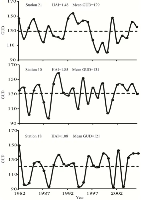
We implemented the GUD detection method (Eqs. 1 and 2) to the remaining 17 gauging stations, and estimated their GUD values. For illustration we have presented the results for three stations that are located at the northern (station 18), middle (station 10) and southern (station 21) parts of the study area, and have different HAI values (their locations being denoted in Fig. 4 by big circles). The resulting annual time series of GUD values for these three stations are presented in Fig. 5 for the years 1982 to 2006. They show that annual GUD values can vary over a wide range – 90 to 160 (day of the year, or DOY) – and that there does not appear to be much concurrence between the temporal patterns between the three gauge locations. Whereas Fig. 5 presented illustrative results of GUD variability in time, the GUD values also exhibit con-siderable spatial (regional) variability. In order to illustrate this, in Fig. 6 we present the spatial pattern of the 25-yr mean GUD values across the region, with the mean GUD estimated from the NDVI data falling in the range of 116 to 137 (DOY) among the 17 gauging stations. Both of these results show that GUD values in this region exhibit considerable spatial (regional) and temporal (inter-annual) variability.

[image:6.595.44.285.400.478.2]

(7)

29

[image:7.595.323.529.60.258.2]

1

Fig. 5. Temporal pattern of Green-up Onset Date (GUD) at stations numbered 21, 10, and 18.

[image:7.595.48.286.65.401.2]

2

Fig. 5. Temporal pattern of GUD at stations numbered 21, 10, and 18.

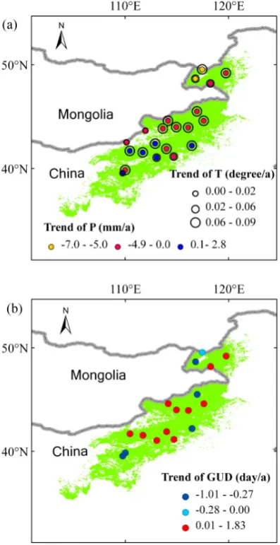
over the past 25 yr, the spatial and temporal trends in GUD are highly variable, suggesting that grass green-up in this re-gion may be influenced by factors other than the thermal con-dition, the most important of which is the water condition.

We illustrate this using data taken from one station within the study region. Figure 9 presents the time series of (smoothed) NDVI, air temperature, (smoothed) precipitation and also modeled soil moisture for station 10 for two con-secutive years, 1997 and 1998. The estimated GUDs from the NDVI data were 133 and 128 DOY, respectively, and are marked on the figure as vertical lines. In 1997, as can be seen in Fig. 8a, the soil moisture was already at a high value since March (perhaps due to carry-over from the previous year), but the temperature was too low for green-up until it hit a threshold, so the dominant control in 1997 may have been temperature. In 1998, shown in Fig. 8b, the temperature was uniformly high in April, yet the grass did not green up until the accumulation of soil moisture due to precipitation rose up and remained high consistently, which suggests that the dom-inant control in 1998 was in fact water (soil moisture). These two examples illustrate the competing controls on GUD, al-though this kind of evaluation is very subjective and time

30

1

Fig. 6. The spatial pattern of 25-year averaged Green-up Onset Date (GUD) of the stations.

2 Fig. 6. The spatial pattern of 25-yr averaged GUD of the stations.

consuming. Could there be an alternative way to determine the dominant controls that mimic the same decision-making processes or rules that grasses possibly adopt during their green-up phase? In the next section we assess the power of the environmental indices proposed earlier to capture the un-derlying controls objectively and make prior predictions. 3.3 Soil moisture vs. precipitation as the basis for a

water index

The time series of SMSO, PSO and TSO for station 10 ob-tained using the estimation procedure described in Sect. 2.4 are presented in Fig. 9 for illustration, along with the corre-sponding GUD values estimated from the NDVI data. These results indicate, for station 10, that the PSO values lie mostly above the GUD values (with very little overlap), whereas the SMSO and TSO values seem to fluctuate above and below the GUD values, with considerable overlap. On the basis of these results, we speculate that in this case the SMSO and TSO indices are more appropriate indices to explain the inter-annual shifts of GUD, and that the precipitation-based index does not have much explanatory power to account for the effect of water availability in relation to the soil-moisture-based index.

(8)

31 1

2

Fig. 7. (a)Trend of air temperature and precipitation in Inner Mongolia from 1982 3

to2006; (b) Trend of Green-up Onset Date (GUD) in Inner Mongolia from 1982 to 4

2006. 5

Fig. 7. (a) Trend of air temperature and precipitation in Inner Mon-golia from 1982 to 2006; (b) trend of GUD in Inner MonMon-golia from 1982 to 2006.

stronger, with a coefficient of determination of 0.52, whereas the correspondence between GUD and PSO as a function of HAI is rather week, with a coefficient of determination of only 0.02. This result shows that the soil-moisture-based index (SMSO) is superior to the precipitation-based index (PSO) as a measure of water availability for capturing ob-served GUD variations.

3.4 Regression results based on dominant thermal/ hydrological indices

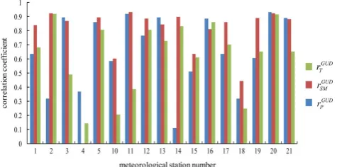
[image:8.595.68.267.64.450.2]

The regression results obtained for the 17 stations using the multiple regression procedure described in Section 2.5 are shown in Fig. 11. The averaged r_SMGUD and r_PGUD val-ues over the 17 stations are, respectively, 0.879 and 0.809, which are higher than the averaged correlationr_TGUD(0.791) based on temperature dominance. Figure 11 also indicates

Fig. 8. Annual series of NDVI, simulated soil moisture, precipita-tion and air temperature of 1997 (a) and 1998 (b) at staprecipita-tion num-ber 10 (the captions J to D in the x-axis stands for January to December).

[image:8.595.308.544.64.459.2]

(9)

33 1

Fig. 9. Time series of SMSO (Soil Moisture Spring green-up Onset date), PSO 2

(Precipitation Spring green-up Onset date), TSO (Thermal Spring Onset date), and GUD 3

(Green-up Onset Date) at station number 10. 4

Fig. 9. Time series of SMSO, PSO, TSO, and GUD at station number 10.

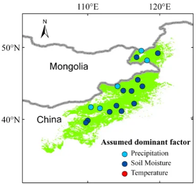
the 17 stations. Even though the water condition is the dom-inant factor in controlling grass green-up in Inner Mongolia

on average, in reality it is indeed possible that the dominant

factor may shift inter-annually between water and tempera-ture. Can the same environmental indices considered here be used to predict this inter-annual variability of the alternating controls? This is a question that will be addressed in our fu-ture work.

4 Discussion and conclusions

Vegetation phenophases, such as spring vegetation green-up, could be influenced by several external factors, of which ther-mal and water conditions are the two most important ones. The thermal condition is always represented by air tempera-ture, whereas in past remote sensing studies the water condi-tion has been represented by precipitacondi-tion, not soil moisture, although soil moisture is more directly related to vegetation growth and phenology. To explore the relationships between the environmental factors (e.g., temperature, precipitation) and vegetation green-up, it has been common to accumu-late these indicator variables over a given, fixed time span; this is not reasonable physically and contributes to poor pre-dictability. Although one could pick out the dominant factor subjectively retroactively after the fact, there is a lack of an objective way to determine the dominant factors that control phenological behavior.

This paper was motivated by the need to overcome gaps in predictive understanding the environmental controls un-derpinning vegetation green-up. Soil moisture at a daily time step was estimated over the study region through regional simulations with the distributed VIC model, which provided the means to explore the role of soil moisture directly. Two spring onset dates, SMSO and PSO, were defined in a way similar to the TSO defined by Shen et al. (2011). For each of these three indices, an optimal time span was estimated through a maximizing process as a way of converting the influence of a hydro/thermal condition to an index that esti-mates a potential GUD, which makes it possible to determine the dominant factor automatically and objectively.

34

[image:9.595.48.286.64.168.2]

1

Fig. 10. Trend of correlations between GUD (Green-up Onset Date) and PSO

2

(Precipitation Spring green-up Onset date)/SMSO (Soil Moisture Spring green-up

3

Onset date) among meteorological stations along a gradient of HAI (the solid circle is

4

the correlation between GUD and PSO, the hollow triangle is the correlation between

5

GUD and SMSO).

6

y = 0.1317x + 0.1783 R² = 0.0228

y = 0.8206x - 1.0717 R² = 0.5164

-0.8 -0.6 -0.4 -0.2 0 0.2 0.4 0.6 0.8

0 0.5 1 1.5 2 2.5

co

rr

el

a

ti

o

n

c

o

ef

fi

c

ie

n

t

HAI GUD vs. PSO

GUD vs. SMSO

Fig. 10. Trend of correlations between GUD and PSO/SMSO among meteorological stations along a gradient of HAI (the solid circle is the correlation between GUD and PSO, the hollow triangle is the correlation between GUD and SMSO).

[image:9.595.309.547.65.199.2]

35 1

Fig. 11. Correlation coefficients between NDVI-derived GUD (Green-up Onset Date) and 2

regressed GUDs by assuming different dominant indices among the meteorological stations, 3

green represents the assumption of temperature as dominant control, red and blue represent 4

that of soil moisture and precipitation respectively. 5

Fig. 11. Correlation coefficients between NDVI-derived GUD and regressed GUDs by assuming different dominant indices among the meteorological stations: green represents the assumption of temper-ature as dominant control, and red and blue represent that of soil moisture and precipitation, respectively.

[image:9.595.310.548.271.389.2]

(10)

[image:10.595.67.268.61.251.2]

36 1

Fig. 12. The spatial pattern of assumed dominant factor based on which could get the 2

best regression of Green-up Onset Date in Inner Mongolia. 3

Fig. 12. The spatial pattern of assumed dominant factor based on which could get the best regression of GUD in Inner Mongolia.

of this, the study showed that the soil-moisture-based index was superior to the one based on precipitation. A hydrologi-cal model operating at finer space shydrologi-cales would therefore be an improvement, and its pursuit is left for further research. Alternatively, recent advances in remote sensing suggest that they might provide a new method for regional soil moisture monitoring, e.g., microwave remote sensing. However, the depth of penetration of these remote sensing instruments is a concern. For example, the AMSR-E instrument measures soil moisture over the upper 5 cm of soil (at most) (Rebel et al., 2012), whereas the root zone for grasses over which they extract soil moisture is of the order of 10 cm. These are areas requiring further research.

During the estimation of the various indices (e.g., SMSO) it was found that there was considerable variability in the accumulation time spans between different stations, even though the vegetation type is the same everywhere. This may be due to differences in drainage rates in these locations, which can be caused by differences in topography and soil texture that the vegetation may have acclimatized to. Differ-ences may also be caused by the presence or absence of a water table, exhibiting longer memory, which the vegetation may be able to draw on. These issues require further eco-hydrological investigation.

As to the regression/prediction ability, we compared our results with that of the other researchers. The determina-tion coefficient of the regression by Shen is about 0.28 for grassland in Qinghai-Tibetan Plateau (Shen et al., 2011), and that by Yu et al. (2003) are 0.54 and 0.87 for typical steppe and desert steppe in eastern central Asia. The determination coefficient is 0.78 in our study when assuming soil mois-ture as the dominant variable. Since the regression regime, variables and accumulation periods are quite different in the

studies, the regression ability comparison needs insightful investigation.

Besides soil moisture and temperature that were explored in this study, there could be many other factors that could contribute to the variability of the GUD, such as irradiance, nutrients and oxygen. More detailed investigations at the lo-cal level will be needed to explore their roles, relative to the roles of soil moisture and temperature.

Acknowledgements. This research was funded by the National

Science Foundation of China (NSFC 51179084, 51190092, 51222901), the special foundation of the Ministry of Water Resources, China (Project No. 201001004), and the foundation of the State Key Laboratory of Hydroscience and Engineering of Tsinghua University (2012-KY-03). Their support is greatly appreciated.

Edited by: S. Thompson

References

Cayan, D. R., Kemmerdiener, S. A., Dettinger, M. D., Caprio, J. M., and Peterson, D. H.: Changes in the onset of spring in the western United States, B. Am. Meteorol. Soc., 82, 399–415, 2001. Chen, J., J¨onsson, P., Tamura, M., Gu, Z., Matsushita, B., and

Ek-lundh, L.: A simple method for reconstructing a high-quality NDVI time-series data set based on the Savitzky-Golay filter, Re-mote Sens. Environ., 91, 332–344, 2004.

Czikowsky, M. J. and Fitzjarrald, D. R.: Evidence of seasonal changes in evapotranspiration in eastern U.S. hydrological records, J. Hydrometeorol., 5, 974–988, 2004.

Do, F. C., Goudiaby, V. A., Gimenez, O., Diagne, A. L., Diouf, M., Rocheteau, A., and Akpo, L. E.: Environmental influence on canopy phenology in the dry tropics, Forest Ecol. Manage., 215, 319–328, 2005.

Holdridge, L. R.: Determination of world plant formations from simple climatic data, Science, 105, 367–368, 1947.

Idso, S. B., Jackson, R. D., and Reginato, R. J.: Extending the “de-gree day” concept of plant phenological development to include water stress effects, Ecology, 59, 431–433, 1978.

Jolly, W. M. and Running, S. W.: Effects of precipitation and soil water potential on drought deciduous phenology in the Kalahari, Global Change Biol., 10, 303–308, 2004.

Julien, Y. and Sobrino, J. A.: Global land surface phenology trends from GIMMS database, Int. J. Remote Sens., 30, 3495–3513, 2009.

Lambers, H., Chapin III, F. S., and Pons, T. L.: Plant Physiology Ecology, 2nd Edn., Springer Science + Business Media, LLC, New York, 2008.

Liang, X., Lettenmaier, D. P., Wood, E. F., and Burges, S. J.: A simple hydrologically based model of land surface water and en-ergy fluxes for general circulation models, J. Geophys. Res., 99, 14415–14428, 1994.

Piao, S., Friedlingstein, P., Ciais, P., Zhou, L., and Chen, A.: Ef-fect of climate and CO2changes on the greening of the Northern

(11)

Rebel, K. T., de Jeu, R. A. M., Ciais, P., Viovy, N., Piao, S. L., Kiely, G., and Dolman, A. J.: A global analysis of soil mois-ture derived from satellite observations and a land surface model, Hydrol. Earth Syst. Sci., 16, 833–847, doi:10.5194/hess-16-833-2012, 2012.

Reed, B. C., Brown, J. F., VanderZee, D., Loveland, T. R., Mer-chant, J. W., and Ohlen, D. O.: Measuring phenological variabil-ity from satellite imagery, J. Veg. Sci., 5, 703–714, 1994. Seghieri, J., Vescovo, A., Padel, K., Soubie, R., Arjounin, M.,

Boulain, N., de Rosnay, P., Galle, S., Gosset, M., Mouctar, A. H., Peugeot, C., and Timouk, F.: Relationships between climate, soil moisture and phenology of the woody cover in two sites lo-cated along the West African latitudinal gradient, J. Hydrol., 375, 78–89, 2009.

Sheffield, J. and Wood, E. F.: Characteristics of global and regional drought, 1950–2000: Analysis of soil moisture data from off-line simulation of the terrestrial hydrologic cycle, J. Geophys. Res., 112, D17115, doi:10.1029/2006JD008288, 2007.

Shen, M., Tang, Y., Chen, J., Zhu, X., and Zheng, Y.: Influ-ences of temperature and precipitation before the growing sea-son on spring phenology in grasslands of the central and east-ern Qinghai–Tibetan Plateau, Agr. Forest Meteorol., 151, 1711– 1722, 2011.

Shinoda, M., Ito, S., Nachinshonhor, G. U., and Erdenetsetseg, D.: Phenology of Mongolian Grasslands and Moisture Conditions, J. Meteorol. Soc. Jpn., 85, 359–367, doi:10.2151/jmsj.85.359, 2007.

Sparks, T. H., Jeffree, E. P., and Jeffree, C. E.: An examination of the relationship between flowering times and temperature at the na-tional scale using long-term phenological records from the UK, Int. J. Biometeorol., 44, 82–87, 2000.

Thompson, S. E., Harman, C. J., Konings, A. G., Sivapalan, M., Neal, A., and Troch, P. A.: Comparative hydrology across AmeriFlux sites: The variable roles of climate, veg-etation, and groundwater, Water Resour. Res., 47, W00J07, doi:10.1029/2010WR009797, 2011.

Wang, J. Y.: A critique of the heat unit approach to plant response studies, Ecology, 41, 785–789, 1960.

Wang, X., Piao, S., Ciais, P., Li, J., Friedlingstein, P., Koven, C., and Chen, A.: Spring temperature change and its implication in the change of vegetation growth in North America from 1982 to 2006, P. Natl. Acad. Sci., 108, 1240–1245, 2011.

Weaver, S. E., Tan, C. S., and Brain, P.: Effect of temperature and soil moisture on time of emergence of tomatoes and four weed species, Can. J. Plant. Sci., 68, 877–886, 1988.

Xie, Z., Yuan, F., Duan, Q., Zheng, J., Liang, M., and Chen, F.: Regional parameter estimation of the VIC land surface model: Methodology and application to river basins in China, J. Hy-drometeorol., 8, 447-468, 2007.

Yang, X., Mustard, J. F., Tang, J., and Xu, H.: Regional scale phenology modeling based on meteorological records and re-mote sensing observations, J. Geophys. Res., 117, G03029, doi:10.1029/2012JG001977, 2012.

Ye, S., Yaeger, M., Coopersmith, E., Cheng, L., and Sivapalan, M.: Exploring the physical controls of regional patterns of flow du-ration curves – Part 2: Role of seasonality, the regime curve, and associated process controls, Hydrol. Earth Syst. Sci., 16, 4447– 4465, doi:10.5194/hess-16-4447-2012, 2012.

Yu, F., Price, K. P., Ellis, J., and Shi, P.: Response of seasonal vege-tation development to climatic variations in eastern central Asia, Remote Sens. Environ., 87, 42–54, 2003.

Yuan, F., Xie, Z., Liu, Q., Yang, H., Su, F., Liang, X., and Ren, L.: An application of the VIC-3L land surface model and remote sensing data in simulating streamflow for the Hanjiang River basin, Can. J. Remote Sens., 30, 680–690, 2004.

Zhang, L. and Liang, Z.: Plant physiology, Science Press, Beijing, 2007.