https://doi.org/10.5194/hess-23-2439-2019 © Author(s) 2019. This work is distributed under the Creative Commons Attribution 4.0 License.
Using MODIS estimates of fractional snow cover area to improve
streamflow forecasts in interior Alaska
Katrina E. Bennett1,2,a, Jessica E. Cherry1,2,3, Ben Balk4, and Scott Lindsey3
1International Arctic Research Center, University of Alaska Fairbanks, Fairbanks, Alaska, 99775, USA 2Water and Environmental Research Center, University of Alaska Fairbanks, Fairbanks, Alaska, 99775, USA 3Alaska Pacific River Forecast Center, Anchorage, Alaska, 99502, USA
4Deltares USA, Silver Spring, Maryland, 20910, USA
acurrent address: Earth and Environmental Sciences, Los Alamos National Lab, Los Alamos, NM, 87545, USA
Correspondence:Katrina E. Bennett ([email protected]) Received: 27 February 2018 – Discussion started: 9 May 2018
Revised: 7 February 2019 – Accepted: 12 March 2019 – Published: 21 May 2019
Abstract. Remotely sensed snow cover observations pro-vide an opportunity to improve operational snowmelt and streamflow forecasting in remote regions. This is particu-larly true in Alaska, where remote basins and a spatially and temporally sparse gaging network plague efforts to under-stand and forecast the hydrology of subarctic boreal basins and where climate change is leading to rapid shifts in basin function. In this study, the operational framework employed by the United States (US) National Weather Service, includ-ing the Alaska Pacific River Forecast Center, is adapted to integrate Moderate Resolution Imaging Spectroradiometer (MODIS) remotely sensed observations of fractional snow cover area (fSCA) to determine if these data improve stream-flow forecasts in interior Alaska river basins. Two versions of MODIS fSCA are tested against a base case extent of snow cover derived by aerial depletion curves: the MODIS 10A1 (MOD10A1) and the MODIS Snow Cover Area and Grain size (MODSCAG) product over the period 2000–2010. Ob-served runoff is compared to simulated runoff to calibrate both iterations of the model. MODIS-forced simulations have improved snow depletion timing compared with snow telemetry sites in the basins, with discernable increases in skill for the streamflow simulations. The MODSCAG fSCA version provides moderate increases in skill but is similar to the MOD10A1 results. The basins with the largest improve-ment in streamflow simulations have the sparsest streamflow observations. Considering the numerous low-quality gages (discontinuous, short, or unreliable) and ungauged systems throughout the high-latitude regions of the globe, this
re-sult is valuable and indicates the utility of the MODIS fSCA data in these regions. Additionally, while improvements in predicted discharge values are subtle, the snow model better represents the physical conditions of the snowpack and there-fore provides more robust simulations, which are consistent with the US National Weather Service’s move toward a phys-ically based National Water Model. Physphys-ically based mod-els may also be more capable of adapting to changing cli-mates than statistical models corrected to past regimes. This work provides direction for both the Alaska Pacific River Forecast Center and other forecast centers across the US to implement remote-sensing observations within their opera-tional framework, to refine the representation of snow, and to improve streamflow forecasting skill in basins with few or poor-quality observations.
1 Introduction
4◦C in winter and 1.9◦C annually from 1949 to 2011 (Stew-art et al., 2013). Snowpack extents in Alaska have decreased over time by 18 % (1966–2012) due to an earlier snow melt, while snowpack duration has also decreased (SWIPA, 2012). Changes in temperature and snow are also affecting frozen ground and leading to permafrost thaw – the temperature of the permafrost near Fairbanks, Alaska, has risen by 2–4◦C from 1930 to 2003 (Slater and Lawrence, 2013; Koven et al., 2013). Rivers in Alaska have been observed to be changing as a result of an intensified or stronger hydrologic cycle that could lead to an increase in peak flows in the North Amer-ican high latitudes (Cohen et al., 2012; Huntington, 2006; Rawlins et al., 2010; Serreze et al., 2011). Riverine breakup dates have been noted to be occurring earlier (Cooley and Pavelsky, 2016; Lesack et al., 2014; Muhammed et al., 2016). Extreme events are also changing; annual maximum stream-flow trends indicate that Alaskan riverine systems are experi-encing streamflow declines, while minimum flow trends are largely increasing (Bennett et al., 2015). All of these shifts are leading to increased streamflow variability (Stuefer et al., 2017), which has strong impacts on the infrastructure and economy of Alaska, and the Arctic as a whole (Instanes et al., 2016), leading to a substantial task in terms of observ-ing, understandobserv-ing, mitigatobserv-ing, and adapting to these effects. The Far North (Arctic and subarctic) is also rapidly develop-ing its hydroelectric water resources, unlike the contiguous US, and needs accurate decision support for managing this infrastructure (Cherry et al., 2017; Sturm et al., 2017).
A challenge for scientists attempting to accurately repre-sent the impacts of climate change on the Alaskan hydro-sphere is the vast territory, complex landscape, and sparse ob-servational network. Alaskan hydrologic systems suffer from large uncertainties in various data inputs, and thus require care when attempting to simulate hydrologic water balance components with skill. For example, precipitation measure-ments are of very poor quality in winter (Cherry et al., 2005, 2007; Groisman et al., 2014) and river stage and discharge measurements by automated gages do not read accurately when ice is present in the river. Reducing these uncertain-ties is important, as they will reduce the value of model out-put (Magnusson et al., 2015; Slater et al., 2013; Clark et al., 2017) and the results cannot provide actionable guidance on water resource management (Stocker et al., 2013). In addi-tion, the variability in landscape (i.e., forest cover, topog-raphy, discontinuous permafrost) and climate across Alaska requires robust modeling techniques to account for potential climate-driven shifts. This adaptable approach is increasingly important as the National Oceanic and Atmospheric Admin-istration (NOAA) National Weather Service (NWS) devel-ops the National Water Model (NWM) framework, a multi-scale water prediction model in operations over the contigu-ous US (NOAA, 2017). Temperature index models, based on the most reliable climate forcing, are often presumed to per-form better than other models for regions with highly vari-able landscapes and a sparse network (Hock, 2003; Stahl
et al., 2006). Alternatively, a skillfully calibrated concep-tual model may provide a better representation of hydrologic responses because the underlying model is reliant upon pa-rameterizations rather than observations that lack spatial and temporal consistency (Franz et al., 2008; Reed et al., 2004).
To deal with the inoperability of stream gages during breakup and in situ snow observations, one technique is to use remotely sensed snow cover areal extent (fSCA) to supplement point observations such as temperature, precip-itation, and streamflow commonly used both as model in-puts and for model calibration and validation (Parajka and Blöschl, 2008). There are two main ways that these data have been used to date: to either directly insert a time series of fSCA data into the model (McGuire et al., 2006; Rodell et al., 2004) or use complex assimilation procedures to filter the snow series and merge it with observational data (Andreadis and Lettenmaier, 2006; Sun et al., 2004; Zaitchik and Rodell, 2009). There is a concern that direct insertion methods are ineffective at improving streamflow models and do not per-form better than uninper-formed models because melt can occur before snow cover drops below 100 % (Clark et al., 2006). In addition, the melt season duration is often short, transition-ing rapidly from snow covered to snow free, although this is largely basin dependent (Clark et al., 2006). Assimilation approaches have yet to be integrated into operational mod-els, in part because of the limited research showing the im-pacts of assimilation on the hydrologic forecast. Other stud-ies have found calibrating models based solely on fSCA val-ues may not improve skill in estimating discharge, and the improvements for in-catchment distributed fSCA estimates do not always result in improved discharge simulation (Franz and Karsten, 2013; Duethmann et al., 2014). However, Liu et al. (2013), Thirel et al. (2013), and Déry et al. (2005) found marked improvements in land surface model output for basins in Alaska when MODIS data were applied.
One approach to improve streamflow forecasts under cli-mate change is to utilize newly developed frameworks to in-gest remotely sensed data on snow cover area into stream-flow models. These newer tools have been adopted by the NWS’s River Forecast Centers (RFCs) and offer an opportu-nity for more advanced streamflow forecasting techniques, including ensemble prediction using variable input and/or forcing data. The Community Hydrologic Prediction Sys-tem (CHPS), brought online in 2012 by the Alaska Pacific River Forecast Center (APRFC), is a test case for this ap-proach. The modeling framework, developed on the Delft-FEWS software platform (Werner et al., 2011), can run many different types of models, but in its current state imple-ments the conceptual Sacramento Soil Moisture Accounting System (SAC-SMA) rainfall–runoff model (Burnash et al., 1973), with snowpack input from the SNOW-17 snow model (Anderson, 2006).
sensed fSCA data for improved streamflow modeling of the interior boreal forest region of Alaska within sparsely and poorly observed river basins that are experiencing shifts as-sociated with a changing climate. We replace the standard areal depletion curve used in SNOW-17 with preprocessed MODIS fSCA grids for snow depletion. Two different ver-sions of MODIS are applied: the MOD10A1 fractional fSCA product, which is the standard MODIS global snow cover product (Hall et al., 2002), and the MOD-Snow Covered Area and Grain size (MODSCAG) fractional fSCA prod-uct, which is a regional product (Painter et al., 2009). The SNOW-17 manual calibration using all model parameters is evaluated, including a tolerance parameter controlling snow cover updates (snow cover tolerance, SCTOL), to simulate a mixed method between direct insertion and more complex data assimilation. Preprocessing, model frameworks, and use of existing parameterizations are thus offered as a means of incorporating remotely sensed information into operational models that can be utilized out of the box by the NWS RFCs. The paper also examines issues around the use of MODIS fSCA in high-latitude boreal forest basins, the interpolation of missing data, and the improvement of streamflow esti-mates by calibrating model parameters used in streamflow forecasting systems across the US (Woo et al., 2008; Prowse et al., 2016).
2 Methods 2.1 Study area
This study was carried out in five adjoining headwater sub-basins of the Tanana River, which is a sub-basin of the Yukon River basin (Fig. 1). The sub-basins include the Chatanika, Upper Chena, Little Chena, Salcha, and Goodpaster basins. The Chatanika River basin (64◦5003700N, 147◦4302300W; Fig. 1) is approximately 950 km2 in size and is oriented predominantly east to west. Only the area upstream of the Caribou–Poker creek confluence is considered in this study. The Chatanika was gaged from 1987 to 2007 but the records are highly discontinuous. The Upper Chena River basin is approximately 2440 km2 and has gage records from 1967 to present. This portion of the basin contains high elevation peaks and rocky outcrops where snow can persist late into the melt season. The Little Chena is 1030 km2and contains the highest proportion of lowlands relative to the other basins; it has been gaged since 1966 to present. The Salcha River basin is a large 5740 km2basin with its gage at the Salchaket Bridge and has the longest historical record of all rivers in this region (1948 to present). The Goodpaster basin is located east of the Salcha and is 1770 km2in size. It has the highest proportion of its basin above 600 m in elevation and has been gaged since 1997 to present. Upper basins are split into sub-basin units with north- and south-facing aspects, with the ex-ception of the Little Chena. There are minor urban and
agri-Figure 1.Map of the five study basins with upper and lower di-visions shown. Alaska SNOTEL sites are shown with numbered black triangles: (1) Fairbanks International Airport; (2) Little Chena Ridge; (3) Munson Ridge; (4) Mt. Ryan; (5) Monument Creek; (6) Teuchet Creek; (7) Upper Chena (Table 2).
culture developments throughout the region, including the town of Fairbanks, which is located downstream of the Lit-tle Chena gage on the main stem of the Chena River. These minor developments have little or no bearing on the hydro-logic response of the headwater systems of Chena basins we examine here. More information on the basins is provided in Table 1.
2.2 Data
The MODIS satellite product (Terra MOD10A1, version 5) provides daily 500 m resolution fractional snow cover area (fSCA) data. It was downloaded from the National Snow and Ice Data Center (Hall and Riggs, 2007; Hall et al., 2006; Riggs et al., 2006) for 2000–2010, and we used the MODIS Re-projection Tool (MRT, USGS, 2011) to preprocess im-agery into an Alaska equal-area conic projected GeoTIFF of fractional fSCA for each sub-basin, which assisted us to cor-rect, in part, the viewing geometry and other issues related to projections of the original MODIS data and the influence these projections have on the MODIS data for Alaska (Dwyer and Schmidt, 2006; Tan et al., 2006). MODSCAG data prod-ucts were obtained from the NASA Jet Propulsion Labora-tory’s Snow Data System Portal (https://snow.jpl.nasa.gov/, last access: 7 May 2019) for the area of interest and prepro-cessed into projected GeoTIFFs to match the spatial proper-ties of the MOD10A1 data. We interpolated cloud- and error-free pixels using a nearest-neighbor approach; only fSCA data from 0 % to 100 % for 1 October to 30 June are ingested into CHPS. Further information on the MODIS data products applied in this study are provided in the Supplement (Supple-ment Sect. S1.1).
[image:3.612.309.551.63.233.2]Table 1.Sub-basin characteristics, including name, sub-basin ID, sub-basin unit, area, elevation mean (range), average monthly temperature,
T, for January (July), average seasonal total precipitation for winter (November–February) (spring, March–June), annual average daily dischargeQ, slope basin units (lower, N is north and S is south∗), and land cover (based on majority cover values∗).T,P, andQcalculated from the 2000–2010 water years.
Name Sub-basin Sub-basin Area Elevation T P Q Units N/S∗ Land cover
ID unit (km2) (m a.s.l.) (◦C) (mm) (m3s−1) (%) (%)
Chatanika CRSA2 Lower 395 475 −22.5 69 11 42 9 D, 83 C, 4S
at the Steese (228–625) (12.6) (102)
Upper 558 780 −18.5 84 25/33 0 D 76 C, 15 S/
(548–1513) (11.9) (112) 2 D, 47 C, 39 S
Little Chena CHLA2 Lower 802 380 −24.4 70 6 78 16 D, 78 C, 5 S
(141–617) (13.7) (101)
Upper 225 721 −21.0 83 22 5 D, 72 C, 20 S
(584–1230) (11.5) (123)
Upper Chena UCHA2 Lower 973 466 −22.5 52 20 40 9 D, 84 C, 5 S
(223–626) (12.7) (106)
Upper 1462 806 −18.2 72 29/31 2 D, 74 C, 17 S/
(553–1584) (11.6) (120) 10 D, 54 C, 33 S
Salcha SALA2 Lower 1838 421 −23.9 51 44 32 18 D, 69 C, 10 S
(194–624) (13.8) (113)
Upper 3900 924 −19.3 77 33/35 2 D, 63 C, 20 S/
(581–1768) (10.6) (139) 7 D, 50 C, 31 S
Goodpaster GBDA2 Lower 737 734 −20.6 55 14 42 2 D, 84 C, 12 S
(411–967) (11.8) (129)
Upper 1036 1166 −19.3 69 29/29 5 C, 33 D 45 S/
(873–1961) (10.1) (153) 2 D, 24 C, 56 S
∗Only upper units are divided into N and S units. Note: D: deciduous; C: coniferous; S: shrubs.
(Raleigh et al., 2013; Rittger et al., 2013), which do not ac-count for the snow that is blocked from the sensor view. For the MOD10A1 fSCA product, this calculation is based on the viewable gap fraction, or the amount of snow-covered ground between trees that the sensor can see (Liu et al., 2004). This technique, while widely applied, assumes that the viewable gap fraction remains constant through the snowmelt season, which is incorrect as the viewable gap fraction can vary based on a complex number of factors, including forest canopy den-sity, age and class, zenith angle of the sensor, solar zenith angles, topography, and snow loading (Kane et al., 2008; Liu et al., 2008; Molotch and Margulis, 2008; Raleigh et al., 2013; Rittger et al., 2013). To account for some of these is-sues, rather than applying a forest cover product to correct the product itself, the MOD10A1 data are used (Durand et al., 2008). All 2000–2013 1 to 15 March MOD10A1 pixels across interior Alaska are differenced from 100, and then a composite average of all days (n=207) is calculated. While in southeast Alaska some melt may have occurred during this time, the interior Alaska fSCA should still be at 100 % snow covered across most of the region. To account for bare
ground regions such as open, wind-blown rocky faces, val-ues less than 20 % fSCA are removed from the correction. The standard division by viewable gap fraction, whereFveg
is the tree cover percentage, SCAfadj(henceforth referred to
simply as fSCA) is the fSCA adjusted for canopy cover, and SCAf is the unadjusted SCA data (Eq. 1).
SCAfadj=
SCAf
1−Fveg
(1)
This formulation is applied as a static adjustment to each SCA pixel in all days and years. For MODSCAG, the daily vegetation fractional product provided with the data prod-uct is utilized, resulting in a dynamic adjustment for each SCA pixel in all days and years. In both cases, the results are constrained to 100 % fSCA when exceeded. We did not in-clude any cloud corrections or additional interpolation meth-ods (Dozier et al., 2008; Morriss et al., 2016).
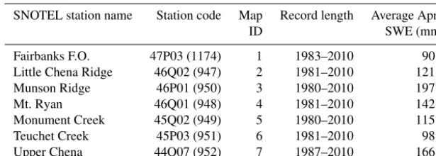
Table 2.SNOTEL stations, map identification, length of record, and observed average snow water equivalent (SWE) used for validation of modeled SWE results. Average April SWE is calculated for the entire period of record.
SNOTEL station name Station code Map Record length Average April
ID SWE (mm)
Fairbanks F.O. 47P03 (1174) 1 1983–2010 90.2
Little Chena Ridge 46Q02 (947) 2 1981–2010 121.5
Munson Ridge 46P01 (950) 3 1980–2010 197.3
Mt. Ryan 46Q01 (948) 4 1981–2010 142.7
Monument Creek 45Q02 (949) 5 1980–2010 115.3
Teuchet Creek 45P03 (951) 6 1981–2010 98.5
Upper Chena 44Q07 (952) 7 1987–2010 166.5
based on the US Geological Survey (USGS) gaging record database. The exception to this is the Chatanika River basin, where observed discharge is generated based on once-a-day stage readings from a Cooperative Network observer. These daily stage readings are converted to mean daily dis-charge using the APRFC’s rating curve for the river. As-pect and elevation were calculated using the 30 m US Ge-ological Survey’s National Elevation Dataset (NED), up-dated for the region in 2012 (Gesch et al., 2002). Seven snow telemetry (SNOTEL) sites are utilized to compare sim-ulated snow water equivalent (SWE) with observed data (Ta-ble 2, NRCS 2013). SNOTEL SWE is downloaded from the National Resource Conservation Service (NRCS) snow pil-low data repository (https://www.wcc.nrcs.usda.gov/legacy/ ftp/cdbs/snotel/cards/alaska/, last access: 7 May 2019).
Potential evapotranspiration (PET) estimates are provided by the APRFC based on an assessment of historical poten-tial evapotranspiration from pan evaporation data and Thorn-thwaite estimates (Anderson, 2006). These data are used to develop a general linear relationship between PET and ele-vation to estimate average monthly PET values for a generic low-elevation site. The APRFC uses the low-elevation PET values to derive monthly estimates for the mean elevation of each sub-basin as a coefficient,C(Eq. 2).
C=0.9−[(elevation−304.8)·0.000353], (2) where elevation represents elevation (m). For example, if the catchment mean elevation is 716 m, the coefficient is 0.75. Finally, a monthly PET adjustment factor is applied to ac-count for vegetation changes during the year. The result is an evapotranspiration demand estimate that is used in the SAC-SMA model, described in the next section.
2.3 Models
The SNOW-17 and the SAC-SMA models are run by the APRFC in an operational framework referred to as CHPS. CHPS is built upon the Delft Flood Early Warning System (FEWS), developed by Deltares (Werner at al., 2013). The CHPS system is briefly described in Sect. S1.2.
2.3.1 SNOW-17
The SNOW-17 snow model is a single-layer snow model that calculates snow accumulation and ablation using empirical formulae to estimate heat and liquid water storage, liquid wa-ter throughflow, and snowmelt (Anderson, 1976). The model is designed for river forecasting and has been used opera-tionally by the NWS RFCs since the mid-1970s. The only input requirements for SNOW-17 are temperature and pre-cipitation (winds are accounted for but not input as observa-tions), at the model time step (6 h). There are 12 parameters in the SNOW-17 model, including the areal snow depletion curve; sensitive or “major” parameters control the model out-puts while less sensitive or “minor” parameters have little impact on the model output (Table 3; He et al., 2011).
SNOW-17 determines the division between rain and snow using the rain–snow elevation (RSNWELEV) module. RSNWELEV uses a defined lapse rate (6◦C 1000 m−1)to
represent the saturated adiabatic lapse rate, which is com-monly applied to determine the air temperature threshold that results in rain turning to snow (PXTEMP; Table 3; Ander-son, 2002; Clark et al., 2011). This temperature threshold is related to an elevation and is passed to SNOW-17; the per-cent area above and below that elevation is determined from a defined area elevation curve. Multiplying these percentages by the precipitation thus defines the proportion of precipita-tion falling as snow or rain in the basin. Non-rain snowmelt (mm) is determined from air temperature minus the base-line temperature at which melt occurs (MBASE; set to 0◦C), weighted by a seasonably variable melt factor that is calcu-lated using an oscillating sine curve that varies between the minimum (MFMIN) and maximum (MFMAX) melt factors for 21 December and 21 June (mm◦C−16 h−1). These values
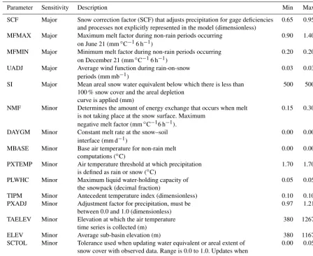
Table 3.SNOW-17 model parameters. Sensitivity indicates whether a parameter has a major or minor influence on model output. Minimum (Min) and maximum (Max) parameter values used in the model simulations. When min and max values are the same the parameter did not vary.
Parameter Sensitivity Description Min Max
SCF Major Snow correction factor (SCF) that adjusts precipitation for gage deficiencies 0.65 0.95 and processes not explicitly represented in the model (dimensionless)
MFMAX Major Maximum melt factor during non-rain periods occurring 0.90 1.40
on June 21 (mm◦C−16 h−1)
MFMIN Major Minimum melt factor during non-rain periods occurring 0.20 0.20
on December 21 (mm◦C−16 h−1)
UADJ Major Average wind function during rain-on-snow 0.03 0.03
periods (mm mb−1)
SI Major Mean areal snow water equivalent below which there is less than 500 500 100 % snow cover and the areal depletion
curve is applied (mm)
NMF Minor Determines the amount of energy exchange that occurs when melt 0.15 0.30 is not taking place at the snow surface. Maximum
negative melt factor (mm◦C−16 h−1).
DAYGM Minor Constant melt rate at the snow–soil 0.00 0.00
interface (mm d−1)
MBASE Minor Base air temperature for non-rain melt 0.00 0.00
computations (◦C)
PXTEMP Minor Air temperature threshold at which precipitation 1.70 1.70
is defined as rain or snow (◦C)
PLWHC Minor Maximum liquid water-holding capacity of 0.05 0.05
the snowpack (decimal fraction)
TIPM Minor Antecedent temperature index (dimensionless) 0.10 0.10
PXADJ Minor Adjustment factor for precipitation, must be 0.97 1.21
between 0.0 and 1.0 (dimensionless)
TAELEV Minor Elevation at which the air temperature 380 1267
time series is collected (m)
ELEV Minor Average sub-basin elevation (m) 380 1167
SCTOL Minor Tolerance used when updating water equivalent or areal extent of 0.00 0.05 snow cover with observed data. Range is 0.0 to 1.0. Updates when
|simulated−observed|>tolerance×observed (dimensionless)
model using parameters that define the lapse rate at time of maximum or minimum temperature.
A simplified energy balance method is used to calculate melt from rain on snow using the following assumptions; the Stefan–Boltzmann constant is used to estimate incoming longwave radiation, negligible shortwave radiation, and 90 % relative humidity, and wind speed is accounted for by adjust-ing for the average value of the wind duradjust-ing rain-on-snow events using the parameter UADJ (mm hPa−16 h−1). Heat content within the snowpack is calculated based on a gradi-ent between air temperature and the near-surface snowpack temperature index to determine the heat flow direction when melt is not occurring. Depending on the near-surface snow-pack temperature index, more or less weight is assigned to temperatures from previous time intervals to represent deeper or shallower snowpack temperatures.
The snow heat deficit is either negative or positive; the rate of heat loss or gain is based on the amount of energy
exchange that occurs when melt is not taking place at the snow surface (negative melt factor; NMF; mm◦C−16 h−1), which is weighted by MFMAX to account for seasonal vari-ations in pack heat translation. Heat can also be translated from the ground to the snow using a parameter that controls the daily melt volume at the interface between snow and soil, and is assumed to occur continuously through the snow sea-son (DAYGM). When the snowpack is at peak water-holding capacity (PLWHC) and is isothermal at 0◦C, the snow is ripe and any excess water entering the snow will flow through it as outflow. Water movement through a ripe pack is attenu-ated or lagged based on the empirical formula derived from lysimeter studies (Anderson, 2006).
2.3.2 fSCA in SNOW-17
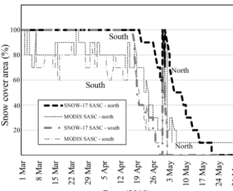
Figure 2.Snow cover area (SCA, %) for the Upper Chena River basin north slope from SNOW-17 and from MODIS in March to May 2010. Large decreases in the MODIS SCA are observed com-pared to the SNOW-17 SCE.
ground melt, and rainfall on bare ground occur (Anderson, 2002; Fig. 7.4.3). The ADC not only represents areal extent of snow cover, but also accounts for slope, aspect, and differ-ences in vegetative cover (i.e., open versus closed sites; An-derson, 2002; Fig. 7.4.3). In the baseline model simulation, the areal extent of snow cover was calculated from a lookup table (Anderson, 2002; Fig. 8) that defines the ADC and re-lates it to the ratio of SWE to either (a) the maximum value of SWE that occurred during snow accumulation or (b) a pa-rameter (SI) that represents the areal SWE at which 100 % snow cover exists (referred to as the areal index). The ADC in the baseline model simulation is applied as follows: when snow accumulates, the snow cover is set to 100 %, and it stays at this value until it falls below SI or the maximum SWE value, whichever is smaller. If new snow totaling greater than 0.2 mm h−1falls onto bare ground, 100 % snow cover is as-sumed until 25 % of the new snow has melted. For Alaska, several different ADC configurations are used depending on whether slopes are south versus north facing, or in upper-versus lower-elevation basins. The basins in this study used the same ADC for upper south, upper north, and lower sub-basin units since they have similar orientations within a sim-ilar geographic region. Only the Little Chena uses a different ADC for its upper basin, as no north–south aspect split is used in this basin. For all other model simulations, the ADC was replaced by areal extent of snow cover derived from the two MODIS fSCA data sets (Fig. 2). Other parameter set-tings used to alter the impact of the MODIS fSCA data in SNOW-17 are described in Sect. S1.3.
2.3.3 SAC-SMA
The SAC-SMA model is a conceptual rainfall–runoff model that simulates streamflow from observed input precipitation and PET (Burnash et al., 1973). SAC-SMA has been widely applied by the NWS to estimate streamflow runoff in basins across the US. The model moves water into either an up-per or lower storage zone that conceptually represent soil in-terception or deep groundwater storage. Inin-terception water in the upper zone flows to the lower zones via downward percolation, or it can run off directly or via interflow when the upper zone layers become saturated and the precipitation rate exceeds downward percolation. Lower zone water can be held in tension storage and contribute to baseflow runoff slowly over time, or can run off more quickly over shorter durations. Drainage from the upper and lower zones follows gravity drainage and is governed in part by both water de-livery from the upper zone and soil moisture in the lower zone. Tension water is driven by potential evapotranspiration and diffusion, with a fraction of the lower zone unavailable for potential evapotranspiration as it is considered below the rooting zone.
A unit hydrograph model is used to adjust runoff timing for each lumped basin in the SAC-SMA model. Each sub-basin has its own unit hydrograph to translate the runoff through the channel system to the gage location. Simple rou-tines sum the unit hydrograph outputs to calculate simulated streamflow at the basin outlet. While downstream basins in-corporate routing models to move water from upstream to downstream basins, this study focuses on headwater basins so no routing models are needed.
2.4 Calibration
Several calibration procedures were undertaken for this project: the baseline calibration and the two MODIS data set calibrations. The baseline calibration effort updated the SAC-SMA–SNOW-17 model parameters to the 2000–2010 years used in this study, as they had previously been adjusted by APRFC to 1970–2003 historical data. The two MODIS man-ual calibrations used the updated baseline to adjust param-eters and generate statistics. Calibration entailed using both visualizations of streamflow hydrographs from 2006 to 2010 and monthly statistics from the entire period of record for ultimate parameter selection.
the observed melt trajectory impacted by the MODIS fSCA data. To complete this simple, physically realistic calibra-tion approach only the parameters MFMAX and TAELEV were adjusted. Further details of the calibration efforts are described in Sect. S1.4.
2.5 Validation
For validation purposes, statistics from 2000 to 2005 are pro-vided for all basins except the Chatanika. The Chatanika basin was calibrated from 2000 to 2004 and validated from 2005 to 2010 to make use of the better data quality and avail-ability during the first 5 years of the study. Statistics used to evaluate model success are based on five main objective functions and monthly average daily model output. The first two of these criteria are standard in NWS RFC calibration approaches and are provided in the CHPS statistical out-put. These statistics were used for evaluation during the cal-ibration: total volume bias as a percent (PBIAS, %) and the correlation coefficient (R, unitless). Three additional objec-tives were added for further validation of the results, Nash– Sutcliffe efficiency (NSE, unitless), the mean absolute error (MAE, m3s−1), and the root-mean-squared error (RMSE, m3s−1). Statistics were run only for April, May, and June to focus on the changes to the snowmelt season; March is not included because generally river ice melts and breaks up in interior Alaska in March; thus any differences in statis-tics would be indicative of changing winter conditions rather than changes in spring snowmelt timing or volume.
3 Results
3.1 Baseline model results
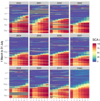
The APRFC SAC-SMA–SNOW-17 baseline model esti-mates of streamflow in the Alaskan interior river basins for the 11-year period of record indicate that these basins are captured with skill (Table 4). The Chatanika basin is prlematic given the limited quality and quantity of the ob-served streamflow data, as noted in the statistics below for each objective function. For all of the five basins analyzed, the daily average bias for the period of record is ±3 % or less. Daily correlation coefficients (R, unitless) are equal to or greater than 0.84 and higher for the four basins with qual-ity observed data, while the Chatanika basin is 0.70. NSE (unitless) daily values are also above 0.60 for all basins ex-cept the Chatanika, which is 0.18 due to the noise in the observed data values. Daily mean absolute error statistics are below 10 m3s−1for all basins except the Salcha, which is 15.89 m3s−1 owing to its long discharge record. RMSE ranges from 3.5 m3s−1 (Chatanika) to 33 m3s−1 (Salcha). Across all basins, fSCA is variable by elevation zones and years (Fig. 3). Upper-elevation areas tend to have 100 % fSCA, while middle to lower areas often begin the year with 75 % fSCA or less. The very lowest-elevation zone
ap-pears to have slightly higher fSCA values than two adjacent higher-elevation zones (Fig. 3). Some years have a markedly late melt out, with high variability across all elevation bins. Lower-elevation zones tend to melt out in early April, while the upper regions of the basins hold snowpack weeks or months into the subarctic spring (Fig. 3).
3.2 SAC-SMA model MODIS calibrations
Calibrated SNOW-17 parameters for the APRFC and MOD10A1 simulations resulted in increased MFMAX for the north-facing aspect in two sub-basin units and increased TAELEV for the north slopes (Table 5) compared to the baseline APRFC SAC-SMA–SNOW-17 simulation. In some sub-basin units, TAELEV was set to be equal for the north and south slopes. MFMAX for the Chatanika’s lowland sub-basin increased and TAELEV at the north sub-sub-basin was in-creased, while TAELEV was decreased for the south sub-basin unit. MFMAX in the Upper Chena north was un-changed and TAELEV was equalized for both south and north sub-basin units. The Little Chena sub-basin parameters were altered by setting MFMAX equal to its maximum rec-ommended value for forested regions (1.4; Anderson, 2002; Table 7-4-1) for the upper and lower sub-basins and by in-creasing TAELEV 100 m greater than the elevation for both sub-basins. TAELEV for Salcha and Goodpaster were dif-ferenced by 100 m for the north and south sub-basin units, and the northern sub-basin MFMAX for Goodpaster was in-creased slightly. Goodpaster’s lower basin MFMAX was re-duced by a small amount. Although these changes may ap-pear minor, MFMAX is highly sensitive during the melt sea-son and therefore these changes have a substantial effect on the MODIS fSCA forced snowmelt trajectory at these sites (Anderson, 2006).
In the MODSCAG simulations, values for MFMAX were increased slightly for the north sub-basin units for all basins. TAELEV values were adjusted slightly in Upper Chena, Salcha, and Little Chena basins (Table 6), but were not al-tered from the baseline run in Chatanika. In the Goodpaster basin, the TAELEV value for the south sub-basin unit was decreased. NMF was altered slightly for both MODIS sim-ulations to account for different snow densities and ther-mal conductivities of snow on south and lowland sites ver-sus north aspects. Snow density (gm cm−3)is generally low in interior Alaska river basins; based on analysis of field data from the Caribou Poker Creek basin, snow density on the sites is approximately 0.20 gm cm−3and is slightly
Table 4.April–May–June monthly calibration (Cal), validation (Val), and the period of record (Per., 1999–2010) statistics (MAE: mean ab-solute error (m3s−1); NSE: Nash–Sutcliffe efficiency (unitless); PBIAS: flow bias (%);R: correlation coefficient (unitless); and RMSE: root-mean-squared error (m3s−1)) for APRFC, MOD10A1, and MODSCAG modeled discharge for all basins. Statistically significant (pvalue < 0.05)Rvalues are shown in italics. Note that the calibration and validation years are not the same for all catchments.
APRFC MOD10A1 MODSCAG
Stat Cal Val Per Cal Val Per Cal Val Per
CRSA2 MAE 3.96 4.73 3.07 3.39 4.66 2.96 3.37 4.22 2.87
NSE 0.10 −0.87 −0.04 0.28 −0.82 0.03 0.29 −0.53 0.11
PBias −17.28 −25.48 −13.08 −16.37 −26.83 −13.07 −16.13 −25.71 −13.27
R 0.61 0.19 0.58 0.69 0.21 0.61 0.69 0.33 0.64
RMSE 5.17 7.24 4.31 4.62 7.15 4.17 4.60 6.54 4.00
CHLA2 MAE 1.85 2.88 1.57 2.00 2.84 1.59 2.09 2.47 1.52
NSE 0.74 0.58 0.81 0.73 0.60 0.81 0.66 0.64 0.82
PBias 4.29 4.84 −2.32 −4.14 −0.65 −5.06 0.56 3.12 −2.84
R 0.88 0.87 0.93 0.86 0.84 0.92 0.82 0.85 0.92
RMSE 2.44 3.46 2.20 2.49 3.38 2.20 2.82 3.21 2.18
UCHA2 MAE 9.12 8.22 5.34 9.15 8.01 5.40 8.75 8.82 5.37
NSE 0.71 0.62 0.81 0.63 0.65 0.80 0.69 0.64 0.81
PBias 16.76 0.39 0.21 10.46 −4.59 −1.05 14.42 −0.48 −0.10
R 0.87 0.85 0.91 0.81 0.84 0.91 0.85 0.85 0.91
RMSE 10.64 12.43 8.43 11.93 11.97 8.68 11.05 12.15 8.44
SALA2 MAE 17.66 21.93 12.31 19.2 24.81 12.94 17.25 23.4 12.45
NSE 0.69 0.63 0.80 0.63 0.53 0.78 0.71 0.60 0.80
PBias 17.21 −14.98 0.35 9.85 −19.07 −1.28 15.18 −15.77 −0.27
R 0.89 0.83 0.90 0.82 0.78 0.88 0.89 0.81 0.90
RMSE 21.10 30.24 19.27 23.32 34.20 20.53 20.56 31.57 19.47
GBDA2 MAE 7.00 3.91 3.62 6.57 5.28 3.93 6.45 4.21 3.63
NSE 0.45 0.90 0.84 0.55 0.83 0.82 0.47 0.86 0.83
PBias 28.10 −11.17 1.46 14.41 −17.60 −1.56 25.89 −12.19 0.83
R 0.88 0.96 0.92 0.89 0.95 0.91 0.91 0.95 0.92
RMSE 10.05 5.05 5.66 9.09 6.72 6.04 9.81 5.96 5.78
Table 5.SNOW-17 parameters for the MOD10A1 calibration. North (N), south (S), upper (U), and lower (L) sub-basins are described. For each sub-basin, the first column indicates the parameter value in the APRFC calibration and the second column indicates the parameter value used in the MODIS calibration. Bold values indicate where the MODIS value differs from the APRFC value.
Parameter Sensitivity N S L N S L U L
CRSA2 UCHA2 CHLA2
MFMAX Major 1.00 1.00 1.40 1.40 1.00 1.40 0.90 0.90 1.40 1.40 1.00 1.00 0.90 1.40 1.30 1.40 NMF Minor 0.30 0.15 0.30 0.20 0.30 0.20 0.30 0.15 0.30 0.20 0.30 0.20 0.20 0.20 0.20 0.20
TAELEV Minor 665 865 1088 988 474 474 708 908 1002 908 465 465 720 820 380 480
SCTOL Minor 0.05 0.00 0.05 0.00 0.05 0.00 0.05 0.00 0.05 0.00 0.05 0.00 0.05 0.00 0.05 0.00
SALA2 GBDA2
[image:9.612.57.539.566.699.2]Figure 3.Snow cover area (%) based on MOD10A1 SCA average across all watersheds divided into elevation zones. The years 2000 to 2010 are shown, with the mean of all years in the final panel. Elevation zones are 1=100–200 m, 1–6, progressing in 200 m increments from 200 to 1200 m, 7=1200–2000 m. Grey areas indicate dates when there is no SCA information (i.e., cloud cover, missing sensor data).
Table 6.SNOW-17 parameters for the MODSCAG calibration. North (N), south (S), and lower (L) basins are described. For each sub-basin, the first column indicates the parameter value in the APRFC calibration and the second column indicates the parameter value used in the MODIS calibration. Bolded values indicate where the MODIS value differs from the APRFC value.
Parameters Sensitivity N S L N S L U L
CRSA2 UCHA2 CHLA2
MFMAX Major 1.00 1.20 1.40 1.40 1.00 1.20 0.90 1.00 1.40 1.40 1.00 0.90 0.90 0.90 1.30 1.20 NMF Minor 0.30 0.15 0.30 0.20 0.30 0.20 0.30 0.15 0.30 0.20 0.30 0.20 0.30 0.20 0.30 0.20
TAELEV Minor 665 665 1088 1088 474 474 708 702 1002 902 465 465 720 720 380 580
SCTOL Minor 0.05 0.00 0.05 0.00 0.05 0.00 0.05 0.00 0.05 0.00 0.05 0.00 0.05 0.00 0.05 0.00
SALA2 GBDA2
MFMAX Major 0.90 1.00 1.40 1.40 1.00 11 0.90 1.00 1.40 1.40 1.00 0.90 NMF Minor 0.30 0.15 0.30 0.20 0.30 0.20 0.30 0.15 0.30 0.20 0.30 0.20
TAELEV Minor 823 923 1123 1023 420 420 863 863 1267 1163 734 734
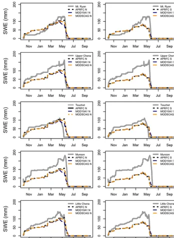
[image:10.612.52.550.556.700.2]Figure 4.Simulated SWE (mm) versus SNOTEL SWE (grey line) for APRFC (solid black line), MOD10A1 (blue dashed line), and MOD-SCAG (orange dotted line) for October 2000 to September 2001. The Upper Chena River basin north slope is shown in the left panels, and the south slope is shown in the right panels.
3.3 fSCA and SWE
Compared to the APRFC simulations, the MODIS simula-tions have less snow cover on the north-facing slopes and more on the south-facing slopes (Fig. 4; the average Upper Chena River basin unit results for 2001 plotted against the SNOTEL stations are shown as an example). Differences be-tween the two simulations become discernable in late Jan-uary as a result of the different calibrations of the SNOW-17
sites: Mt. Ryan, Munson, and Upper Chena. The APRFC and MOD10A1 runs melt out later than the MODSCAG fSCA north unit and the MODSCAG estimates are closer to the APRFC simulations in volume, although all simulations ter-minate on the same approximate day for the northern sub-basins.
The SNOTEL sites are mostly located at upper elevations (Mt. Ryan, 850 m; Munson, 940 m) compared to the SNOW-17’s∼800 m elevation parameter and thus illustrate condi-tions exhibited at high-elevation northern sites in the basin. Mt. Ryan, in particular, does not build a snowpack early in the season, perhaps owing to its open, mountainous, and pre-sumably windy environment. The SNOW-17 model is run over a lumped area so there is a mix of site conditions that act to smooth and reduce the volume of SWE; hence the comparison between SNOTEL SWE and SNOW-17 mod-eled SWE is inherently qualitative as opposed to quantitative (Molotch and Bales, 2005). The lower-elevation SNOTEL sites, Teuchet and Little Chena, show earlier melt out than is seen in either the model output or the MODIS data sets. There is stronger coherence in the response of the northern sites as opposed to the southern sites. In the south sub-basin units, the MODIS simulations melt out later, with MOD-SCAG again having the latest melt, similar in timing to the high-elevation stations.
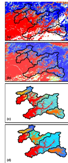
The areal extent of snow cover varies across the basins in both simulations. The preprocessed gridded MOD10A1 fSCA illustrated for 15 May 2001 is shown in Fig. 5a and the MODSCAG fSCA is shown in Fig. 5b for the basins. The high-elevation snowpack (blue) is present within the upper basin regions but the pack is largely gone in the valleys and lower basin reaches. This translates into the lumped average fSCA estimates shown in Fig. 5c and d, which illustrate how CHPS ingests and converts the gridded MODIS fSCA for the sub-basin units. North and south sub-basin units are dif-ferentiated in the upper sub-basin units (see Table 1) but not at other locations because both aspects have begun to melt by this date (as opposed to early in the melt period when the south slopes would have comparatively less fSCA than the north slopes). MODSCAG has less cloud cover interaction in this scene (Fig. 5b) and this results in slightly higher val-ues of fSCA (Fig. 5d).
[image:12.612.357.498.65.402.2]SWE estimates for MOD10A1 (Fig. 6a), MODSCAG (Fig. 6b), and the difference between the MODIS (both versions) and APRFC runs (Fig. 6c and d) is shown for 15 May 2001. Sub-basin units can be clearly differentiated in these plots, which illustrate the range of SWE values from 0 to 25 mm in the lowland regions to 125 mm in the upper headwaters. The MODSCAG data have an average fSCA value of 0.51 (51 %) and SWE is 45 mm, whereas the MOD10A1 has an average of 0.45 (45 %) fSCA and an aver-age of 54 mm SWE, very small differences overall although sub-basin to sub-basin the variation between the products is notable. The difference plots highlight the fact that MODIS tends to have lower SWE values compared to the APRFC
Figure 5.Study area snow cover area in the CHPS model frame-work for(a)MOD10A1 and(b)MODSCAG, where white is either missing or cloud covered, and elevation-averaged (lumped by ele-vation) snow cover extent based on(c)MOD10A1 and(d) MOD-SCAG. Values range from 10 % to 100 % snow cover. All panels show results for 15 May 2001.
SNOW-17 model simulations on the north-facing slopes and higher values on the south-facing slopes. The APRFC tends to have lower SWE estimates for the lowland regions, al-though this is more true for MOD10A1 than MODSCAG (Fig. 6c, d).
3.4 Streamflow estimates
Figure 6.Study area basin SWE (mm) estimates in CHPS model framework for(a)MOD10A1 and(b)MODSCAG and the percent-age difference between both SWE estimates and the APRFC run (for positive values, MODIS is higher, for negative values, APRFC is higher;candd). All panels show results for 15 May 2001.
Chatanika and Goodpaster systems during the calibration pe-riod, while they perform similarly or slightly worse during the validation and period of record in most of the basins ex-cept the Chatanika. The MODSCAG run exhibits better per-formance compared to the APRFC run during the calibra-tion periods in the Chatanika, Salcha, and Goodpaster basins, while the validation period statistics showed improvement for the Chatanika, Little Chena, and Upper Chena basins. Overall, improvements in skill are observed for the MODIS simulations in the Chatanika and Goodpaster basins, the vali-dation period for Upper Chena, and the calibration period for Goodpaster (Table 4).
The calibration, validation, and whole period of record re-sults illustrate that for the poorly performing basins, MOD-SCAG (and MODMOD-SCAG with SCTOL=0.25) tends to do slightly better versus APRFC in the calibration/validation time where improvements are also made for MOD10A1, while both MODIS versions perform nearly identically over
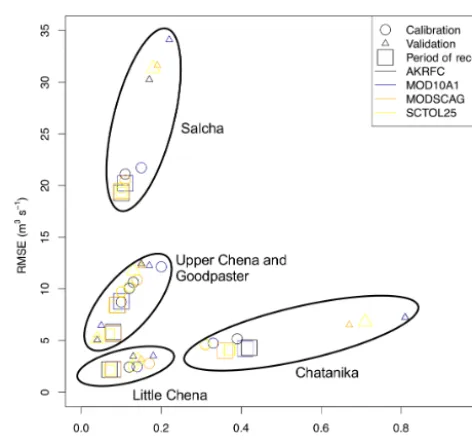
Figure 7.Monthly RMSE (m3s−1)plotted against 1−Rfor cal-ibration (open circles), validation (open triangles), and period of record (open squares). Values are given for each of the five basins. Black: APRFC; blue: MOD10A1; orange: MODSCAG; and yel-low: MODSCAG with SCTOL=0.25. Results cluster by basin, as indicated by the oval groupings on the plot.
the 11-year period (Fig. 7). This can also be observed from the analysis presented in Fig. 8 for all five basins. Figure 8 illustrates that the MODSCAG results tend to follow more closely (and are hence more constrained) with the APRFC results, while the MOD10A1 product has more scatter. How-ever, the differences from observations are similar between the two products.
[image:13.612.97.239.63.411.2]Figure 8.Percent difference between observed streamflow and that modeled using APRFC plotted against modeled MOD10A1 (blue) and MODSCAG (orange) for March–June from 2000 to 2010. The APRFC percent difference (yaxis) is plotted against the MOD10A1 and MODSCAG percent differences (xaxis). The 1:1 line is illus-trated on the plots for reference.
better than the APRFC, which over-simulates streamflow on average, and both products perform similarly well. Stream-flow simulations for the Upper Chena, Salcha, and Good-paster systems match observations more closely, on aver-age. This also is clear from the averages across basins and years; the MODSCAG simulations match observed stream-flow, while the MOD10A1 product underestimates runoff during the mid-May to early June period (Fig. 9, last panel). The year-to-year variability illustrates similar results to the long-term averages for each basin (Supplement).
3.5 Other integration methods
Two methods were applied to integrate the MODIS data into CHPS. One method involved interpolating between miss-ing data values, changmiss-ing the number of interpolated days from 1 to 11 to investigate how changing the value impacted
Table 7.Comparison between RMSE (%) and NSE (in brackets) for April–May–June using SCTOL values of 0.25, 0.50, and 0.75. Absolute differences are calculated from the MODSCAG base run. Cal: calibration; Val: validation; Per: period of record.
SCTOL CRSA2 UCHA2 CHLA2 SALA2 GBDA2
0.25 Cal. −2 18 12 19 −2
(−0.03) (0.13) (0.08) (0.16) (−0.03)
0.50 −10 −9 −1 8 12
(−0.29) (−0.05) (−0.01) (0.07) (0.03)
0.75 −4 4 2 6 5
(−0.08) (0.02) (0.01) (0.03) (0.01)
0.25 Val. −11 19 15 18 −6
(−0.17) (0.14) (0.1) (0.15) (−0.06)
0.50 −15 −14 −2 6 12
(−0.45) (−0.08) (−0.02) (0.06) (0.03)
0.75 −8 3 2 6 4
(−0.15) (0.01) (0.01) (0.03) (0.01)
0.25 Per. −10 21 12 19 −7
(−0.15) (0.15) (0.08) (0.16) (−0.08)
0.50 −11 −20 −12 7 17
(−0.34) (−0.12) (−0.09) (0.06) (0.04)
0.75 −7 1 −1 6 4
(−0.13) (0.01) (0) (0.03) (0.01)
[image:14.612.308.546.118.354.2]Figure 9.Upper Chena River basin streamflow: observed (grey line), simulated with APRFC (black dotted line), simulated with MOD10A1 (blue dashed line), and simulated with MODSCAG (orange dashed line) for all years (2000–2010, 15th of the month shown onx axis). Streamflow is shown as specific discharge, with discharge divided by area of the basins (km). The mean of all stations is shown in the final panel.
4 Discussion
Results illustrate that streamflow in interior Alaska can be simulated with skill using conceptual, semi-lumped hydro-logic models, even without the use of gridded observations of MODIS fSCA. However, if the initial streamflow observa-tions are of poor quality (i.e., Chatanika River basin), apply-ing gridded observations of MODIS fSCA in the models will generate streamflow estimates as good as or better than esti-mates based on SNOW-17’s areal depletion curve. However, as the climate shifts, conceptual, semi-lumped models may not be representative of process changes that will likely oc-cur as the Arctic warms (Clark et al., 2017). As fully process-based models are challenging to run in Arctic environments, where high-quality data are temporally and spatially sparse, using conceptual models parameterized with as many ob-servations as possible represents a bridge between the fully process-based models and conceptual approaches to hydro-logic modeling.
systems that are changing quickly due to climate shifts and increased occurrences of extreme events (Bennett and Walsh, 2015; Bennett et al., 2015).
The goal of this work was, in part, to undertake a simple application of inserting preprocessed MODIS fSCA into the CHPS operational framework to simulate streamflow across basins in interior Alaska. The preprocessing of MODIS data for insertion into the model, which included the MOD10A1 and MODSCAG data products, along with the CHPS areal averaging, eliminated some of the issues related to cloud cover and missing data, as noted in results provided in Liu et al. (2013), who assimilated Air Force Weather Agency– National Aeronautics and Space Administration Snow Algo-rithm (ANSA) fSCA data for similar stations in the region. For example, the findings in Liu et al. (2013) for the best case indicate NSE improvement for Salcha, Little Chena, and Chena at Fairbanks of 0.30, 0.31, and 0.06. Our study reports comparable NSE improvement values for some sta-tions (Chatanika and Goodpaster) for the months impacted by the adjustments, although the Salcha and Little Chena system differences are closer to those values reported for the raw MODIS data in the study of Liu et al. (2013). The av-eraging approach and use of newly developed tools (ANSA, MODSCAG) applied in both studies appear to produce re-sults slightly superior to those of MOD10A1. Further anal-ysis is required to determine if cloud correction processes, such as those applied in the ANSA study, would act to reduce the impact of pixel shifting that is likely a major problem in Alaska (Arsenault et al., 2014) and improve streamflow esti-mates further. Both studies indicate improved representation of internal snowpack and improvements in streamflow esti-mates for some basins for these new iterations of the MODIS data.
Differences in the streamflow improvements provided by Liu et al. (2013) for the Salcha and Little Chena basin high-light some important variations between the two studies that should be considered. The first is that, as noted by the au-thors, the model-simulated streamflow estimates are biased and thus the improvements reported in the paper are still poor representations of the streamflow (Liu et al., 2013). The question then remains that if a model result without up-dated observations is already skillful, how much better can the model be with added information (which carries its own uncertainty with it)? Perhaps the differences between the dis-tributed model in Liu et al. (2013) versus the lumped models used in this study are adding a buffer to the data improve-ments in the case of this study, and limiting the amount of difference or improvement that MODIS fSCA insertion can provide. Snow cover data appear to be improved at interior Alaska locations within the model when compared to five different SNOTEL stations (Fig. 5), particularly for the melt timing. However, the discharge values improved moderately given MODIS input over the different periods analyzed, and in particular smaller changes are noted over the entire pe-riod of record (Table 4, Figs. 8, 9). For the Chatanika basin,
with limited observed data and poorer streamflow simula-tions however, the improvements are similar to those shown in the Liu study (Liu et al., 2013). These results suggest that skill can be added by introducing new observations when the models are performing poorly due to inadequate or low-quality records. Considering that there are numerous incom-plete and low-quality gages throughout the high-latitude re-gions of the globe, this result is valuable and indicates the utility of the MODIS fSCA data in this regard.
Calibrations performed on the SAC-SMA model were lim-ited in nature and targeted specifically at two parameters ex-hibiting the most influence on improving discharge estimates during the melt season: MFMAX and TAELEV. These pa-rameters control the air temperature and impact snow cover depletion by either increasing or retaining melt. Previously, the APRFC parameters were set to lower MFMAX values. The TAELEV parameter was not equal to the true elevation (ELEV) and set to different values for north and south as-pects. For north-facing upper elevations, TAELEV was less than ELEV so temperatures were lapsed upward to simulate the slower melt rates and cooler conditions. For south-facing aspects, TAELEV was set to greater than ELEV, so tem-peratures were lapsed downward to simulate increased melt from solar influence. Our updated parameterization using the MODIS data required an upward adjustment of these values because the areal depletion curve is no longer controlling the melt rate. Thus, fSCA present on northern, upper-elevation slopes in the late spring must have higher melt rates applied to melt the snow with the correct timing. The primary reason that the areal depletion curves in SNOW-17 differ from one that would be derived from actual measurements of fSCA is that melt rates decline as fSCA declines because the remain-ing snow is usually found in locations where snow melts at a slower rate, such as under canopies or on north-facing slopes (Anderson, 2006).
Therefore, by improving the internal physical processes in the model, the snowmelt timing should improve. However, this might not translate into improved discharge estimates because precipitation and temperature inputs could still be incorrect, and errors in forcing data that generate incorrect water equivalents for snow carry larger uncertainty bounds than that which can be addressed by changing the weighting factors and timing of snowmelt by adjusting fSCA, as under-taken in this study.
For the MOD10A1 calibration, fewer parameters were ad-justed compared to the MODSCAG simulations. The end result is that the MODSCAG data have improved stream-flow simulations compared to the MOD10A1 result. The model parameters require greater adjustment for MODSCAG simulations as a result of the variability between the two data sets compared to the APRFC baseline simulations. The MODSCAG data have a different melt trajectory for northern slopes and hold snow for longer on the south-facing slopes of the Upper Chena River basin, while the MOD10A1 acts sim-ilarly to the APRFC melt trajectory for SWE data (Fig. 4). This region is known to have variable melt timing based on south-facing slopes; therefore the north and south slopes should be differentiated to reflect the physical processes occurring on the warmer south-facing slopes compared to the cold and often permafrost-dominated north-facing slopes (Jones and Rinehart, 2010). Although MODSCAG improve-ment is noted for the Chatanika and Goodpaster basins in the streamflow statistics, the results for both MODIS versions are overall very similar in this region (Fig. 8). This may be due to the different canopy adjustments applied to the data sets or because of the lack of a spectral end member for the boreal forest in MODSCAG (Painter et al., 2009). Regardless, it is not clear that one of these data sets is markedly improving streamflow estimates and it is possible that both approaches could be considerably useful as additional observations of fSCA estimates for the region.
Two other means by which the CHPS framework can be altered to improve streamflow estimates are explored in this work. The interpolation over MODIS missing days can be altered easily in CHPS; however this had only a small ef-fect on the streamflow results. The SCTOL, which allows for interaction between the model and the observed MODIS fSCA data, had an effect on streamflow and therefore may be a useful technique for the RFCs to apply during recali-bration efforts to observed snow cover data. An advantage was noted between the MODSCAG with an SCTOL setting greater than to 0.25. However, the basins with the strongest improvement (Chatanika) over the APRFC simulation did not improve using an SCTOL greater than zero, which was because the baseline model performed so poorly given the weakness of the underlying observed discharge data. There-fore, the RFCs may wish to selectively apply this parame-ter when basins have reliable observed information and the MODIS data can be utilized partially in conjunction with the model ADC and partially on the MODIS fSCA observations.
5 Conclusions
Although complex tools and distributed models are available from the research community and in the CHPS to integrate observed snow cover area data, the RFCs across the US are not, as of writing this paper, using these features in their op-erational river forecasting to estimate floods and droughts. This study focuses on developing tools that can, with a mi-nor amount of testing, be brought into the RFC’s CHPS mod-eling framework and used to improve physical estimates of fSCA across basins of interest. The method integrates infor-mation such as MODIS remotely sensed snow cover into the model framework using a simple calibration approach for the SNOW-17 model, and also provides some input regarding ex-pected improvements and other possible parameters that may be introduced to enrich forecasting and simulation of stream-flow. Our recommendation is to incorporate MODIS data as an interim step. However, in the long run the RFCs should be-gin to use more complex models and data assimilation tools as the move towards the National Water Model proceeds.
In this work, we answer several outstanding questions re-garding the application of MODIS data in the RFC models. Basins with poor-quality streamflow observations benefited from the use of the MODIS fSCA but improvements are also made to the internal snow timing estimates, observed in both the validation against SNOTEL data and also through the calibration that corrected the model parameters to bet-ter reflect the physical differences albet-tering processes occur-ring on north- and south-facing slopes. Overall, minor differ-ences were observed between MOD10A1 and MODSCAG data; however the MODSCAG data provided improvement over MOD10A1 in average streamflow simulations across all basins. We observed limited impact of changing the inter-polation length between missing days, although adjustments based on altering the interaction between the model and the observed MODIS fSCA data did alter streamflow and there-fore are useful during recalibration efforts.
The utility of the MODIS data in CHPS goes beyond im-provements to the streamflow; these tools can be used for a number of internal checks for SWE and fSCA that are cur-rently under way, such as the ingestion of data for ensemble forecasts (NWS, 2012). This study opens the door for inser-tion of parameters via assimilainser-tion alongside developments such as physically based model usage.
understand-ing of Arctic hydrologic processes, process-based modelunderstand-ing approaches are limited in this environment. Therefore, we must apply available conceptual models with calibrations in-formed by observations, including remote sensing tools of SWE and fSCA to examine these effects. In this way, we will be able to define and quantify increasing impacts associ-ated with these changes that lead to multi-scale risk to hydro-ecological systems, not only to the local and state resources, but also regionally and globally.
Data availability. MODIS MOD10A data set is available for download through https://doi.org/10.5067/MODIS/MOD10A1.006 (Hall and Riggs, 2016). MODSCAG data are available via https://snow.jpl.nasa.gov/portal/ (Painter et al., 2009). USGS river gauge data are available for download from https://waterdata. usgs.gov/nwis/rt (USGS, 2019). SNOTEL SWE data are avail-able from https://www.wcc.nrcs.usda.gov/snow/snotel-wereports. html (NRCS, 2019) Mean areal temperature and precipitation 6-hourly data used to run SACSMA/SNOW17 are available via the authors at the Alaska Pacific River Forecast Center.
Supplement. The supplement related to this article is available online at: https://doi.org/10.5194/hess-23-2439-2019-supplement.
Author contributions. All authors were involved in the conception, and development of workflow. KB and BB responsible for develop-ment of software manipulation of CHPS modeling framework. KB and JEC responsible for writing. KB, JEC, and SL contributed to editing process through various stages of the manuscript develop-ment.
Competing interests. The authors declare that they have no conflict of interest.
Acknowledgements. Katrina E. Bennett acknowledges support for this work from the Alaska Climate Science Center, the Natural Sci-ence and Engineering Research Council of Canada, and the DOE Office of Science, Biological and Environmental Research program, Next Generation Ecosystem Experiment, NGEE-Arctic project. Ka-trina E. Bennett, Ben Balk, and Jessica E. Cherry acknowledge support from the GOES-R High Latitude Proving Ground award NA08OAR432075. Thank you to Sarah Boon for reviewing an ear-lier version of this work. The authors thank the Alaska Pacific River Forecast Center staff for their collaborative efforts and the Arctic Region Supercomputer Center for the use of their supercomputer.
Review statement. This paper was edited by Shraddhanand Shukla and reviewed by Stephen Déry, Edward Bair, and one anonymous referee.
References
Arsenault, K. R., Houser, P. R., and De Lannoy, G. J.: Evaluation of the MODIS snow cover fraction product, Hydrol. Process., 28, 980–998, 2014.
Anderson, E. A.: A point energy and mass balance model of a snow cover, NOAA Tech. Rep. NWS 19, Office of Hydrology, National Weather Service, Silver Spring, MD, 150 pp., 1976.
Anderson, E. A.: Calibration of conceptual hydrologic models for use in river forecasting, Office of Hydrologic Development, US National Weather Service, Silver Spring, MD, 372 pp., available at: https://www.nws.noaa.gov/oh/hrl/modelcalibration/ 1.CalibrationProcess/1_Anderson_CalbManual.pdf (last access: 8 May 2019), 2002.
Anderson, E. A.: Snow Accumulation and Ablation Model – SNOW-17, Nat. Weather Serv. NOAA, 44 pp., available at: http://www.nws.noaa.gov/oh/hrl/nwsrfs/users_manual/part2/ _pdf/22snow17.pdf (last access: 17 August 2018), 2006. Andreadis, K. M. and Lettenmaier, D. P.: Assimilating
re-motely sensed snow observations into a macroscale hydrology model, Adv. Water Res., 29, 872–886, https://doi.org/10.1016/j.advwatres.2005.08.004, 2006. Bennett, K. E. and Walsh, J.: Spatial and temporal changes in
in-dices of extreme precipitation and temperature for Alaska, Int. J. Climatol., 35, 1434–1452, https://doi.org/10.1002/joc.4067, 2015.
Bennett, K. E., Cannon, A. J., and Hinzman, L.: Historical trends and extremes in boreal Alaska river basins, J. Hydrol., 527, 590– 607, https://doi.org/10.1016/j.jhydrol.2015.04.065, 2015. Burnash, R. J. E., Ferral, R. L., and McGuire, R. A.: A generalized
streamflow simulation system, Joint Federal-State River Forecast Center, Sacramento, CA, 204 pp., 1973.
Cherry, J. E., Tremblay, L. B., Déry, S. J., and Stieglitz, M.:. Reconstructing solid precipitation from snow depth measure-ments and a land surface model, Water Resour. Res., 41, 1–15, https://doi.org/10.1029/2005WR003965, 2005.
Cherry, J. E., Tremblay, L. B., Stieglitz, M., Gong, G., and Déry, S. J.: Development of the pan-arctic snowfall reconstruction: new land-based solid precipitation estimates for 1940-99, J. Hydrom-eteorol., 8, 1243–1263, https://doi.org/10.1175/2007JHM765.1, 2007.
Cherry, J. E., Knapp, C., Trainor, S., Ray, A. J., Tedesche, M., and Walker, S.: Planning for climate change impacts on hy-dropower in the Far North, Hydrol. Earth Syst. Sci., 21, 133–151, https://doi.org/10.5194/hess-21-133-2017, 2017.
Clark, M. P., Slater, A. G., Barrett, A. P., Hay, L. E., Mc-Cabe, G. J., Rajagopalan, B., and Leavesley, G. H.: As-similation of snow covered area information into hydrologic and land-surface models, Adv. Water Res., 29, 1209–1221, https://doi.org/10.1016/j.advwatres.2005.10.001, 2006. Clark, M. P., Hendrikx, J., Slater, A. G., Kavetski, D., Anderson,
B., Cullen, N. J., Kerr, T., Hreinsson, E. Ö., and Woods, R. A: Representing spatial variability of snow water equivalent in hy-drologic and land-surface models: A review, Water Resour. Res., 47, 1–23, https://doi.org/10.1029/2011WR010745, 2011. Clark, M. P., Bierkens, M. F. P., Samaniego, L., Woods, R. A.,
for physical realism, Hydrol. Earth Syst. Sci., 21, 3427–3440, https://doi.org/10.5194/hess-21-3427-2017, 2017.
Cohen, J. L., Furtado, J. C., Barlow, M. A., Alexeev, V. A., and Cherry, J. E.: Arctic warming, increasing snow cover and widespread boreal winter cooling, Environ. Res. Lett., 7, 014007, https://doi.org/10.1088/1748-9326/7/1/014007, 2012.
Cooley, S. W. and Pavelsky, T. M.: Spatial and temporal patterns in Arctic river ice breakup revealed by automated ice detection from MODIS imagery, Remote Sens. Environ., 175, 310–322, https://doi.org/10.1016/j.rse.2016.01.004, 2016.
Déry, S. J., Salomonson, V. V., Stieglitz, M., Hall, D. K., and Appel, I.: An approach to using snow areal depletion curves inferred from MODIS and its application to land sur-face modelling in Alaska, Hydrol. Process., 19, 2755–2774, https://doi.org/10.1002/hyp.5784, 2005.
Dozier, J., Painter, T. H., Rittger, K., and Frew, J. E.: Time-space continuity of daily maps of fractional snow cover and albedo from MODIS, Adv. Water Res., 31, 1515–1526, https://doi.org/10.1016/j.advwatres.2008.08.011, 2008. Duethmann, D., Peters, J., Blume, T., Vorogushyn, S., and
Günt-ner, A.: The value of satellite-derived snow cover images for calibrating a hydrological model in snow-dominated catch-ments in Central Asia, Water Resour. Res., 50, 2002–2021, https://doi.org/10.1002/2013WR014382. 2014.
Durand, M., Molotch, N. P., and Margulis, S. A.: Merging comple-mentary remote sensing datasets in the context of snow water equivalent reconstruction, Remote Sens. Environ., 112, 1212– 1225, https://doi.org/10.1016/j.rse.2007.08.010, 2008.
Dwyer, J. and Schmidt, G.: The MODIS reprojection tool, in: Earth Science Satellite Remote Sensing, Springer, Berlin, Heidelberg, Germany, 162–177, 2006.
Euskirchen, E., McGuire, A., Chapin III, F., Yi, S., and Thompson, C.: Changes in vegetation in northern Alaska under scenarios of climate change, 2003–2100: implications for climate feedbacks, Ecol. Appl., 19, 1022–1043, https://doi.org/10.1890/08-0806.1, 2009.
Franz, K. J. and Karsten, L. R.: Calibration of a distributed snow model using MODIS snow covered area data, J. Hydrol., 494, 160–175, https://doi.org/10.1016/j.jhydrol.2013.04.026, 2013. Franz, K. J., Hogue, T. S., and Sorooshian, S.: Operational snow
modeling: Addressing the challenges of an energy balance model for National Weather Service forecasts, J. Hydrol., 360, 48–66, https://doi.org/10.1016/j.jhydrol.2008.07.013, 2008.
Gesch, D., Oimoen, M., Greenlee, S., Nelson, C., Steuck, M., and Tyler, D.: The National Elevation Dataset, Photogramm. Eng. Rem. S., 68, 5–11, 2002.
Groisman, P. Y., Bogdanova, E., Alexeev, V., Cherry, J., and Buly-gina, O.: Impact of snowfall measurement deficiencies on quan-tification of precipitation and its trends over northern Eurasia, Ice Snow, 54, 29–43, https://doi.org/10.15356/2076-6734-2014-2-29-43, 2014.
Hall, D. K. and Riggs, G. A.: Accuracy assessment of the MODIS snow product, Hydrol. Process., 21, 1534–1547, https://doi.org/10.1002/hyp.6715, 2007.
Hall, D. K. and Riggs, G. A.: MODIS/Terra Snow Cover Daily L3 Global 500m SIN Grid, Version 6, Snow Cover, Boulder, Colorado USA, NASA National Snow and Ice Data Center Distributed Active Archive Center, https://doi.org/10.5067/MODIS/MOD10A1.006, 2016.
Hall, D. K., Riggs, G. A., Salomonson, V. V., DiGirolamo, N. E., and Bayr, K. J.: MODIS snow-cover products, Remote Sens. Environ., 83, 181–194, https://doi.org/10.1016/S0034-4257(02)00095-0, 2002.
Hall, D. K., Riggs, G. A., and Salomonson, V. V.: MODIS/Terra Snow Cover Daily L3 Global 500m Grid V005, 2000-Daily Up-dates, National Snow and Ice Data Center, Boulder, Colorado USA, 2006.
He, M., Hogue, T. S., Franz, K. J., Margulis, S. A., and Vrugt, J. A.: Characterizing parameter sensitivity and uncertainty for a snow model across hydroclimatic regimes, Adv. Water Res., 34, 114– 127, https://doi.org/10.1016/j.advwatres.2010.10.002, 2011. Hinzman, L. D., Bettez, N. D., Bolton, W. R., Chapin, F. S.,
Dyurg-erov, M. B., Fastie, C. L., Griffith, B., Hollister, R. D., Hope, A., Huntinton, H. P., Jensen, A. M., Jia, G. J., Jorgenson, T., Kane, D. L., Klein, D. R., Kofinas, G., Lynch, A. H., Lloyd, A. H., McGuire, A. D., Nelson, F. E., Oechel, W. C., Osterkamp, T. E., Racine, C. H., Romanovsky, V. E., Stone, R. S., Stow, D. A., Sturm, M. D., Walker, D. A., Webber, P. J., Welker, J. M., Winker, K. S., and Yoshikawa, K.: Evidence and implications of recent climate change in northern Alaska and other Arctic regions, Cli-mate Change, 72, 251–298, https://doi.org/10.1007/s10584-005-5352-2, 2005.
Hinzman, L. D., Deal, C. J., McGuire, A. D., Mernild, S. H., Polyakov, I. V., and Walsh, J. E.: Trajectory of the Arc-tic as an integrated system, Ecol. Appl., 23, 1837–1868, https://doi.org/10.1890/11-1498.1, 2013.
Hock, R.: Temperature index melt modelling in mountain ar-eas, J. Hydrol., 282, 104–115, https://doi.org/10.1016/S0022-1694(03)00257-9, 2003.
Huntington, T. G.: Evidence for intensification of the global water cycle: review and synthesis, J. Hydrol., 319, 83–95, https://doi.org/10.1016/j.jhydrol.2005.07.003, 2006.
Instanes, A., Kokorev, V., Janowicz, R., Bruland, O., Sand, K., and Prowse, T.: Changes to freshwater systems affecting Arctic infrastructure and natural resources, J. Geophys. Res.-Biogeo., 121, 567–585, https://doi.org/10.1002/2015JG003125, 2016. Jones, J. B. and Rinehart, A. J.: The long-term response of stream
flow to climatic warming in headwater streams of interior Alaska, Can. J. Forest Res., 40, 1210–1218, 2010.
Kane, V. R., Gillespie, A. R., McGaughey, R., Lutz, J. A., Ceder, K., and Franklin, J. F.: Interpretation and topographic compensation of conifer canopy self-shadowing, Remote Sens. Environ., 112, 3820–3832, https://doi.org/10.1016/j.rse.2008.06.001, 2008. Karl, T. R., Melillo, J. M., Peterson, T. C., and Hassol, S. J. (Eds.):
Global climate change impacts in the United States, Cambridge University Press, 2009.
Koven C. D., Riley W. J., and Stern, A.: Analysis of per-mafrost thermal dynamics and response to climate change in the CMIP5 Earth system models, J. Climate, 26, 1877–900, https://doi.org/10.1175/JCLI-D-12-00228.1, 2013.
Lesack, L. F. W., Marsh, P., Hicks, F. E., and Forbes, D. L.: Local spring warming drives earlier river-ice breakup in a large Arctic delta, Geophys. Res. Lett., 41, 1560–1567, https://doi.org/10.1002/2013GL058761, 2014.