www.hydrol-earth-syst-sci.net/19/3541/2015/ doi:10.5194/hess-19-3541-2015
© Author(s) 2015. CC Attribution 3.0 License.
Impacts of beaver dams on hydrologic and temperature regimes
in a mountain stream
M. Majerova1, B. T. Neilson1, N. M. Schmadel1, J. M. Wheaton2, and C. J. Snow1
1Utah Water Research Laboratory, Department of Civil and Environmental Engineering, Utah State University, 8200 Old Main Hill, Logan, Utah, 84322-8200, USA
2Department of Watershed Sciences, Utah State University, 8200 Old Main Hill, Logan, Utah 84322-8200, USA
Correspondence to: M. Majerova ([email protected]) and B. T. Neilson ([email protected])
Received: 3 December 2014 – Published in Hydrol. Earth Syst. Sci. Discuss.: 22 January 2015 Revised: 30 June 2015 – Accepted: 2 July 2015 – Published: 11 August 2015
Abstract. Beaver dams affect hydrologic processes, channel complexity, and stream temperature in part by inundating ri-parian areas, influencing groundwater–surface water interac-tions, and changing fluvial processes within stream systems. We explored the impacts of beaver dams on hydrologic and temperature regimes at different spatial and temporal scales within a mountain stream in northern Utah over a 3-year pe-riod spanning pre- and post-beaver colonization. Using con-tinuous stream discharge, stream temperature, synoptic tracer experiments, and groundwater elevation measurements, we documented pre-beaver conditions in the first year of the study. In the second year, we captured the initial effects of three beaver dams, while the third year included the effects of ten dams. After beaver colonization, reach-scale (∼750 m in length) discharge observations showed a shift from slightly losing to gaining. However, at the smaller sub-reach scale (ranging from 56 to 185 m in length), the discharge gains and losses increased in variability due to more complex flow pathways with beaver dams forcing overland flow, increas-ing surface and subsurface storage, and increasincreas-ing ground-water elevations. At the reach scale, temperatures were found to increase by 0.38◦C (3.8 %), which in part is explained by a 230 % increase in mean reach residence time. At the smallest, beaver dam scale (including upstream ponded area, beaver dam structure, and immediate downstream section), there were notable increases in the thermal heterogeneity where warmer and cooler niches were created. Through the quantification of hydrologic and thermal changes at different spatial and temporal scales, we document increased variabil-ity during post-beaver colonization and highlight the need to
understand the impacts of beaver dams on stream ecosystems and their potential role in stream restoration.
1 Introduction
interac-tions can also impact the overall temperature regime (e.g., upwelling zones decrease temperatures below beaver dams; Fanelli and Lautz, 2008; White, 1990). Regardless of this im-plied connection between hydrologic and stream temperature changes due to beaver dam construction, most studies have investigated these changes separately. Furthermore, the tem-poral and spatial scales considered within individual stud-ies vary widely, leading to inconsistent conclusions regarding beaver dam impacts on stream systems (Kemp et al., 2012).
When considering hydrologic influences at the beaver dam scale (which includes the beaver dam structure, the upstream ponded area, and the section below the dam), Briggs et al. (2012) found a connection between streambed morpholo-gies formed upstream of a beaver pond and the hyporheic flow patterns. Similarly, Lautz and Siegel (2006) showed that beaver dams promoted higher infiltration of surface water into the subsurface. Janzen and Westbrook (2011) found en-hanced vertical recharge between the stream and underlying aquifer upstream of dams and longer hyporheic flow paths than those measured in other studies. Nyssen et al. (2011) studied impacts of beaver dams at a larger reach scale and throughout a series of beaver dams; similar to other literature (Gurnell, 1998; Burns and McDonnell, 1998), they found that a series of beaver dams retained water during high flows and increased low flows through drier periods. The authors also assessed that the recurrence interval for major floods in-creased over 20 years and peak flows were dein-creased and delayed by approximately 1 day. In contrast, some argue that while beaver dams affect downstream delivery of water, they provide minimal retention during extreme runoff events (Burns and McDonnell, 1998).
The documented impacts of beaver dams on temperature are more variable. Some studies found that beaver dams and beaver ponds cause overall increases in downstream temper-atures (Andersen et al., 2011; Margolis et al., 2001; Salyer, 1935; McRae and Edwards, 1994; Shetter and Whalls, 1955) with reported values as high as 9◦C during summer months (Margolis et al., 2001). Fuller and Peckarsky (2011) also observed increases in temperatures below low-head beaver dams, but a cooling effect below high-head beaver dams. At the longer reach scale (22 km), Talabere (2002) found no significant influence of beaver dams on stream temperature. A recent literature review regarding the impacts of beaver dams on fish further summarizes such inconsistent findings. Kemp et al. (2012) cited 13 articles that argued beaver dams provided thermal refugia and 11 articles that argued nega-tive impacts from altered thermal regime (i.e., detrimental increases in summer temperatures). Interestingly, this review also pointed out that of the 13 articles claiming temperature benefits of beaver dams, only seven were data driven and the remaining six were speculative. Of the 11 articles showing temperature impairments, only one was data driven while the rest were speculative. Another recent literature review re-garding the effects of beaver activity in stream restoration and management further revealed that a majority of studies
cover small spatial-scale areas (e.g., small reach scales), are mainly qualitative, and many hypotheses are supported only by anecdotal or speculative information (Gibson and Olden, 2014). Particularly in the context of stream management, where beaver have recently been considered as a potential restoration tool (e.g., Utah Division of Wildlife Resources, UDWR, 2010), a more quantitative understanding based on field observations of the hydrologic and thermal impacts of beaver within stream systems is critical.
Variability in hydrologic and thermal responses in streams with beaver dams and the subsequent inconsistent conclu-sions found in the literature highlight the need for more data driven studies across multiple spatial and temporal scales. In an effort to link hydrologic and temperature responses due to beaver dam development, we present data from different spa-tial (reach, sub-reach, and beaver dam) and temporal scales (instantaneous to continuous 3-year time series) that span a period prior to and during the establishment of 10 beaver dams. We illustrate how the development of beaver dams shifts instream hydrologic and thermal responses.
Site description
Curtis Creek, a tributary of the Blacksmith Fork River in northern Utah, drains a portion of the Bear River range. Cur-tis Creek is a first-order perennial mountain stream with in-termittent tributaries. The mountainous watershed includes a combination of hard sedimentary rock; Paleozoic and Pre-cambrian limestone bedrock that is strongly indurated. The valley broadens in the lower portion of Curtis Creek and is primarily dominated by remnant low-angle alluvial fans. The valley bottom is comprised of a mix of longitudinally stepped floodplain surfaces and channels that are both partly confined by coarse-grained alluvial fan deposits with gravel, cobble, boulders and some soil development.
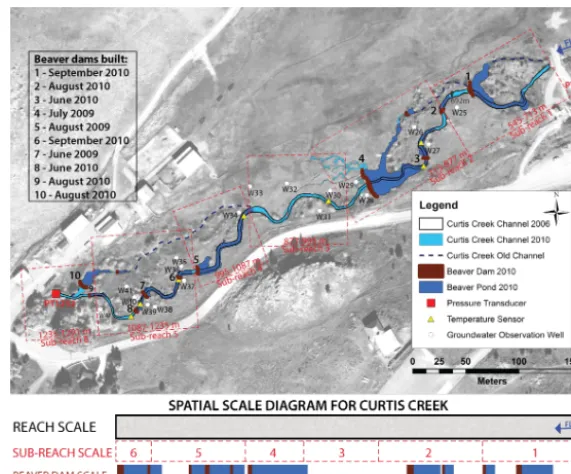
coloniza-Figure 1. Aerial image from 2006 (pre-beaver period) and beaver dams constructed between 2009 and 2010. The main beaver dams are
numbered 1–10 from upstream to downstream and the time of dam construction is noted in the table. The study reach was further divided into six sub-reaches. The spatial scales investigated are illustrated below the map. The most downstream beaver dam and beaver pond are located in the old channel but overlap in the beaver dam scale schematic in this figure. The 2006 channel is outlined in black, while the flowing and ponded water area from 2010 are represented by different shades of blue.
tion began with beaver dam 7 being constructed in the middle of the study reach (Fig. 1). Beaver dams 4 and 5 were also completed during the summer of 2009. New beaver dams (3 and 8) were established early summer 2010 and by the late summer–early fall, dams 2, 6, 9, and 10 were completed. By the end of fall 2010, beaver dam 1 was built at the upstream end of the study reach resulting in a total of 10 beaver dams with an average height of 1 m (measured at the downstream face of a dam as the difference between the channel bot-tom and the top of the dam crest). In addition, two small (less than 0.5 m in height) beaver dams were constructed in the old channel (Fig. 1; dams without numbers). Beaver built seven of their dams using the artificial restoration struc-tures as foundations. By the end of fall 2010, the channel consisted of sections with flowing water (main channel and side channels), ponded water (beaver ponds), and beaver dam structures (Fig. 1). The resulting dam density by 2010 was 13.3 dams km−1.
2 Methods
The field site was originally instrumented with pressure transducers, temperature sensors, and groundwater observa-tion wells to investigate groundwater–surface water interac-tions in the absence of beaver. After 1 year of data collection, beaver colonization occurred within the study reach, chang-ing the objectives of the study. In short, it produced the
per-fect accidental experiment and a unique opportunity to quan-tify fundamental hydrologic and thermal impacts of beaver dam construction on stream systems. In an effort to specifi-cally investigate these impacts, three primary data types were collected over a 3-year period spanning pre- and post-beaver colonization (Table 1; Fig. 1). Flow information was col-lected at the reach (∼750 m in length) and sub-reach scale (between 56 m and 185 m in length) to compare influences of individual beaver dams and cumulative impacts. In addi-tion, groundwater levels were observed within the floodplain of the study reach. To explore the corresponding impacts of dams on thermal regimes, stream temperature data were col-lected and analyzed at the reach, sub-reach, and beaver dam scales. Both the hydrologic and temperature data collection took place over different temporal scales and the frequency varied from instantaneous measurements to continuous data throughout the 3-year period.
2.1 Data collection
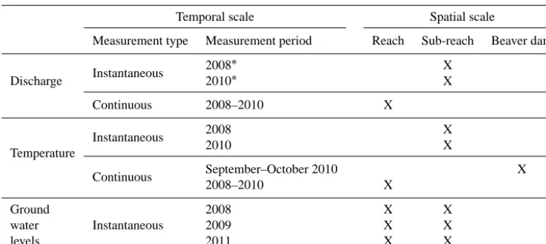
[image:3.612.155.441.65.302.2]Table 1. Discharge, temperature, and ground water level observations made at different spatial and temporal scales throughout the study
reach.
Temporal scale Spatial scale
Measurement type Measurement period Reach Sub-reach Beaver dam
Discharge Instantaneous
2008∗ X
2010∗ X
Continuous 2008–2010 X
Temperature
Instantaneous 2008 X
2010 X
Continuous September–October 2010 X 2008–2010 X
Ground
Instantaneous
2008 X X
water 2009 X X
levels 2011 X X
∗Based on flows calculated from dilution gaging.
upstream, inflow (PT515; Fig. 1) and downstream, outflow study reach limit (PT1252; Fig. 1). Both pressure transduc-ers were installed in the flowing water close to the bank with an average streambed slope of 0.017 and 0.024 for inflow (PT515) and outflow (PT1252), respectively. Water level and temperature were measured at 30 s intervals and 5 min aver-ages were recorded. Discharges were measured at each PT under the full range of flow conditions using the velocity-area method to establish rating curves. The flow velocity was recorded with a Marsh McBirney Inc.® Flo-Mate™ (Model 2000, Frederick, Maryland). The lowest flow measured was 157 L s−1 at PT1252 and the highest flow measured was 1510 L s−1, also at PT1252. To provide a local comparison of hydrologic responses due to beaver activity, continuous discharge data were similarly collected at the bounds of a control reach approximately 535 m long without any beaver activity, located immediately upstream from our study reach (PT0).
The study reach was further divided into six sub-reaches, ranging from 56 to 168 m and numbered sequentially down-stream (Fig. 1). The six sub-reaches spanned individual dams (e.g., sub-reach 4), multiple dams (e.g., sub-reaches 2 and 5), and a non-impounded sub-reach that received surface return flows via small side channels or overland flow from an up-stream beaver pond (sub-reach 3). The boundaries for the sub-reaches were chosen to ensure completely mixed con-ditions necessary for dilution gaging (Schmadel et al., 2010). Dilution gaging was conducted at the sub-reach scale on 16 July 2008 (pre-beaver) and 19 July 2010 (post-beaver) to provide a longitudinal understanding of flow variability. As described within Schmadel et al. (2010, 2014), chlo-ride (from NaCl) was used as a conservative tracer (Zell-weger, 1994) and rhodamine WT was used as a visual indi-cator for a qualitative assessment of mixing. Tracer injection
masses ranged from 600 to 3300 g as NaCl and were var-ied to achieve large enough responses in electrical conduc-tivity above background for dilution gaging and mass recov-ery purposes. Tracer responses were measured following an instantaneous tracer injection starting at the downstream end of the study reach and then moving upstream to individual sub-reach boundaries. Each response was measured with spe-cific conductance (SC) (electrical conductivity normalized to 25◦C as a surrogate to chloride concentrations) at 1 s inter-vals using YSI®sondes (models 600 LS and 600 XLM, Yel-low Springs, Ohio) calibrated in the field. The background SC was corrected to zero (Gooseff and McGlynn, 2005; Payn et al., 2009) and each corrected response was correlated to chloride concentrations with calibration regressions.
To capture changes in groundwater levels throughout the reach, groundwater observation wells were installed in June 2008 (Fig. 1). These wells were constructed of half-inch polyvinyl chloride (PVC), 2 m in length with 40 cm of per-foration covered with 2 mm flexible nylon screen to exclude soil. Elevations and horizontal coordinates were established for individual wells using differential rtkGPS (Trimble®R8, Global Navigation Satellite System, Dayton, Ohio). Ground-water levels were determined by measuring the distance from the top of each well to the groundwater surface level in each well using a Solinst®electronic well sounder (Model 101 Mini, Georgetown, Ontario, Canada). The groundwater levels were measured 4 times in 2008 (June, July (twice), August), 5 times in 2009 (June, July, August (twice), and November), and 4 times in 2011 (April, June, July, and November).
Mas-Table 2. Distance for temperature sensors located upstream and downstream of individual beaver dams (BD) during 2 September–15 October
2010 (Fig. 1).
Beaver Distance from beaver dam Description
dam (m) (period 2 September–15 October) Temperature Temperature
sensor sensor upstream downstream
3 15 9 Upstream sensor was initially in flowing water near the transition to the ponded area and later in slowly flowing water; downstream sensor is at the boundary of flowing and ponded water from BD4.
4 60 49 Upstream sensor is same as BD3 downstream; downstream sensor is in a flowing, well-mixed portion of the channel.
5 81 21 Upstream sensor is in flowing water near the transition to the ponded area; downstream sensor is same as BD7 above.
7 47 9 Upstream sensor is in flowing water near the transition to the ponded area; downstream sensor is same as BD8 above.
8 8 6 Upstream sensor is in flowing water near the transition to the ponded area; downstream sensor is in flowing, well-mixed portion of the channel.
sachusetts) deployed from 2 September to 15 October 2010 (Fig. 1; Tables 1, 2). The temperature sensors were placed in the thalweg of the flowing channel entering the pond to en-sure well-mixed conditions. The sensors downstream from the beaver dams were placed past the scour pool, but in the completely mixed portion of the channel. The temperature sensors were attached to metal stakes, placed in the channel, approximately halfway through the water column. Individ-ual sensors were wrapped in aluminum foil to reduce solar radiation influence in slower moving waters.
The air temperature, relative humidity, solar radiation, wind speed and precipitation data were collected with the meteorological station located within the study reach.
Aerial imagery was used to delineate and compare pre-and post-beaver colonization flowing pre-and ponded water area. Pre-beaver colonization conditions (2006) were cap-tured with high-resolution aerial imagery available through the Utah Automated Geographic Reference Center (AGRC). Post-colonization, NIR (near infrared) and RGB (red-green-blue) aerial imagery were collected using Aggie Air UAVs (Unmanned Aerial Vehicle) in 2010. Aggie Air flights that additionally included thermal aerial images were completed in 2011–2013.
2.2 Data analysis
At the reach scale, the 5 min continuous stage and tem-perature data recorded at the study reach boundaries were averaged to daily values to illustrate changes over the 3-year study period. Data from the winter months were ex-cluded from the analysis because they were influenced by ice buildup around the pressure transducers. Rating curves
were developed from the measured discharges and continu-ous stage in the form (Cey et al., 1998; Rantz, 1982):
Q=aZb, (1)
whereQis the predicted discharge (L s−1),a andb are the regression parameters, andZ is the stage measured by the pressure transducer (m). The parameters,aandb, were esti-mated through nonlinear regression where the minimum sum of squares occurred. Uncertainty in these parameters was as-sessed from values within the associated 95 % joint confi-dence region, which produced the 95 % conficonfi-dence bounds of the rating curve (Schmadel et al., 2010). The error (as 95 % confidence intervals) inQwas subsequently estimated directly from these bounds. The continuous discharge es-timates provided corresponding eses-timates of net change in stream discharge (1Q) at the reach scale (downstream dis-charge minus upstream disdis-charge). To illustrate percent net change (%1Q),1Qwas normalized by upstream discharge (Q at the upstream reach boundary). The net change in stream temperature (1T; downstream temperature minus up-stream temperature) and %1T were also calculated at the reach scale. To determine if meteorological conditions were influencing the water temperature differences between years, we first compared average daily air temperatures for each year through a one-way analysis of variance (ANOVA) (α= 0.05). We then compared daily1T values normalized by air temperature for the days when both water and air temperature were available within each year (α=0.01).
[image:5.612.66.517.97.314.2](Kil-patrick and Cobb, 1985)
Q= M
τ R
0
(C(t )−Cb(t ))dt
= M
τ R
0 C(t )dt
, (2)
whereQis the stream discharge (L s−1),M is the mass of solute tracer injected (mg),C(t )is the tracer concentration (mg L−1),Cb(t )is the background tracer concentration (cor-rected to zero) (mg L−1),tis time (s), andτ is the measure-ment time period from tracer injection to last detection (s). The net1Qwas also estimated from theQat the boundaries of each sub-reach (Fig. 1). The net1Qfor each sub-reach was again normalized by the discharge at the corresponding upstream sub-reach limit resulting in a net %1Qto allow for direct comparison between sub-reaches. Uncertainty in the estimates was quantified using the same technique presented in Schmadel et al. (2010) and provided the 95 % prediction interval around theQand1Qestimates. Tracer mass recov-ery (MR) through each sub-reach was quantified to provide information regarding flow diversions within and possible re-turns to some sub-reaches (Payn et al., 2009):
MR=QD Z
CD(t )dt, (3)
where QD is the discharge at the downstream sub-reach boundary (L s−1), and CD is the recovered tracer concen-tration at the downstream boundary from the injection just above the upstream boundary (mg L−1). In addition, mean residence times (µt) for individual sub-reaches were esti-mated from the first temporal moment or expected value of each recovered tracer response as
µt= τ R
0
t CD(t )dt τ
R
0
CD(t )dt
. (4)
To further understand hydrologic impacts of beaver dam con-struction and to illustrate the channel and groundwater eleva-tion gradient changes over time, these data were grouped by each sub-reach and were evaluated for 2008, 2009, and 2011. The groundwater elevation data collected in 2010 were lim-ited and, thus, the post-beaver colonization period was repre-sented by the 2011 data. Due to the placement of established groundwater observation wells, changes in groundwater over the study period were available for sub-reaches 2, 3, and 5.
The temperature impacts at the beaver dam scale were quantified from the data collected upstream of ponded wa-ters and downstream of individual beaver dams (3, 4, 5, 7, and 8) from fall 2010 (Fig. 1 and Table 2). In the case of beaver dams 7 and 8, the ponded water from beaver dam 8 extended to beaver dam 7. Therefore, we used data upstream of dam 7 and downstream of dam 8. A 24 h moving aver-age was calculated from the data to detect temporal trends
other than diurnal patterns. The net temperature change,1T, for each individual beaver dam was calculated by subtracting the temperature upstream of the beaver dam from the tem-perature downstream of the beaver dam. A positive change represented net warming, while a negative change repre-sented net cooling downstream from the beaver dams. The area of flowing water (represented by the stream channel) and ponded water from the beaver dams was digitized and calculated from the 2006 (pre-beaver conditions) and 2010 (post-beaver colonization conditions) imagery (Table 3). The main channel water volume for pre- and post-beaver dams were also estimated based on one-dimensional HEC-RAS hydraulic model built to replicate the two different states (Ta-ble 3).
3 Results
3.1 Reach-scale responses
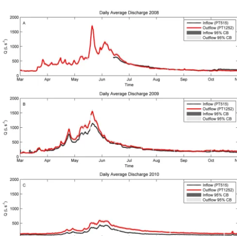
At the reach scale, the average daily discharge (Fig. 2) illus-trates the seasonal variations and changes in flow conditions at the inflow (PT515) and outflow PT1252 for 2008 through 2010. The 2008 and 2009 flows were fairly comparable with peak flows at PT1252 of 1698 and 1549 L s−1, respectively. The 2010 flows were, however, one-third of peak flow in comparison to previous years (592 L s−1 at PT1252). This difference is also illustrated with snow water equivalent and precipitation accumulation from a nearby SNOTEL (Snow Telemetry) site (Fig. S1 in the Supplement). The impacts of beaver dam building activities are directly reflected in the reach-scale flow conditions and in the year-to-year variabil-ity in net1Qand %1Q(Fig. 3). Negative changes indicate a net losing reach while positive values indicate net gains in flow. The daily average value for March–October of 2008 (pre-beaver) was−5.6 L s−1for1Qand−4.4 % for %1Q. As the beaver dams were built and increased in number, the average values of1Qand %1Qincreased to 51.2 L s−1and 13.2 % in 2009 and to 81.2 L s−1and 53.1 % in 2010, respec-tively.
Table 3. Annual change in flow (1Q) and annual percent net change ( %1Q) for the study reach impacted by beaver dams (shown in Fig. 1) and for an adjacent, upstream control reach with no beaver dams present. Change in stream temperature (1T), percent change ( %1T), and area of flowing water and ponded water area for the study reach impacted by beaver dams is listed as well. Change in flow and temperature and their percentages (1Q, %1Q,1T, %1T) were calculated as an average of daily1values for each year (Figs. 3, 5).
2008 2009 2010 Study reach 1Q(L s−1) −5.60 51.20 81.20 (with beaver dams) %1Q −4.40 13.20 53.10
1T (◦C) 0.22 0.17 0.43
%1T 2.10 1.10 4.40 Flowing water area (m2) 1776 – 1211 Ponded water area (m2) 0 – 2830 Water volume (m3) 636∗ – 2449∗ Control reach 1Q(L s−1) −24.30 −55.90 −92.50 (no beaver dams) %1Q −7.70 −19.80 −42.50
∗The water volume is an estimate from a one-dimensional model where pre- and post-beaver dams flow conditions were captured. The 2010 water volume was calculated using discharge of 930 L s−1and includes only main channel water without any side channels or off-channel beaver ponds.
Figure 2. Daily average discharge estimated from continuous
pres-sure transducer records spanning 2008–2010 (a–c). The black-dashed line represents upstream, inflow conditions at PT515 and the red-solid line represents downstream, outflow conditions at PT1252. The individual 95 % confidence intervals around discharge estimates are represented by grey shading. Note that the inflow bounds are very small and are, therefore, not visible in the figure.
The greatest %1Qoccurred at the end of June 2010 reaching approximately 80 % (Fig. 3). This drastic change may be par-tially affected by irrigation patterns in nearby fields during the summer months (mid-May through July), but the gains remain through to November.
Figure 3. (a) Change in discharge over the study reach calculated
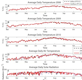
[image:7.612.46.290.303.545.2] [image:7.612.305.549.328.573.2]Figure 4. Average daily temperature (absolute) representing reach-scale responses at inflow (PT515, black-dashed line) and outflow (PT1252,
red-solid line) during (a) 2008, (b) 2009, and (c) 2010. (d) Average daily air temperature and (e) average daily solar radiation show similar weather patterns for all three years.
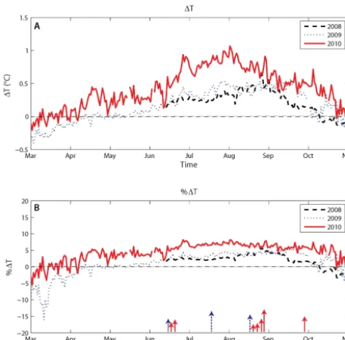
At the reach scale, stream temperatures consistently in-creased during the summer with peaks occurring at the end of July and beginning of August with some periods of cool-ing within the reach in the fall for all 3 years (Fig. 4). Net and percent changes in temperature (1T and %1T) show a warming trend from 2008 to 2010 corresponding to the increase in the number of dams (Fig. 5). In 2008, the aver-age daily1T was 0.22◦C and in 2010 the average1T was 0.43◦C. The average increase from 2008 to 2010, with differ-ences based on the daily1T (not on their yearly averages), was 0.38◦C (%1T =3.8 %). The maximum difference in 1T between these years was 0.77◦C (%1T =8.5 %) and occurred on 1 August (Fig. 5).
The one-way ANOVA for air temperature comparison showed no statistical difference between individual years (p >0.05). Further comparison of daily1T values normal-ized by air temperature showed a significant difference in the daily average values (p <0.01) between years. This suggests that the between year variability in air temperature is not con-trolling the observed1T patterns.
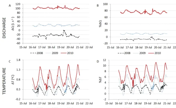
Reach-scale data from a smaller temporal scale (a 5-day period in July) illustrates the links between discharge and temperature patterns associated with beaver dam construc-tion (Fig. 6). Comparison of 1Qand %1Qshow similar trends to those in Fig. 3 (i.e., an increase in the amount of
water gained over the reach each year), but with diurnal pat-terns. The %1Qfor 2010 shows an approximate 80 % in-crease in discharge when compared to 2008 (Fig. 6b). The transformation from losing in 2008 to gaining in 2010 is also more pronounced at this shorter 5-day scale. Similarly, when comparing1T and %1T values there is an average increase of 0.6◦C and 4.6 % from 2008 to 2010, respectively. The data also contain a diurnal pattern with a maximum difference of 1.1◦C (8 %) between 2008 and 2010 (Fig. 6c–d). The1T
values show that the range of temperature differences dur-ing the day doubled in 2010. In 2008, the flowdur-ing water sur-face area was estimated to be 1776 m2with no ponded area (Fig. 1; Table 3). In 2010, the flowing water surface area decreased to 1211 m2with the ponded area covering about 2830 m2. The total water surface area in 2010 had more than doubled.
3.2 Sub-reach scale responses
Figure 5. (a) Reach-scale change in temperature (1T) calculated from temperatures at the reach outflow (PT1252) minus the temper-ature at the reach inflow (PT515). (b) %1T is the percent change relative to the temperature at the inflow location (PT515). Positive values represent warming throughout the reach and negative val-ues represent cooling relative to the upstream inflow temperature at PT515. Arrows represent time of individual beaver dam construc-tion. Blue and red arrows correspond with years 2009 and 2010, respectively, while the arrow size is proportional to size of the dam.
by another 0.34 m from 2009 to 2011. For sub-reaches 3 and 5, median groundwater levels increased by 0.02 and 0.12 m from 2008 to 2009, respectively. From 2009 to 2011, these levels increased further by 0.10 m in sub-reach 3 and by 0.15 m in sub-reach 5. Based on the positive head gradi-ent between groundwater and surface water, sub-reaches 2 and 3 are primarily gaining. However, sub-reach 5 is gener-ally neutral in 2008 and is more commonly losing surface water in 2009 and 2010 (Figs. 7; S2). The head gradients from the cross section of wells in sub-reach 5 show an in-crease in groundwater elevation over time and generally de-pict a positive gradient on one side of the channel and nega-tive gradient on the other (Fig. S2).
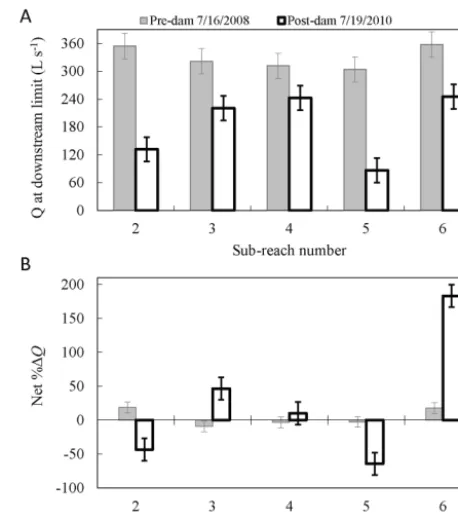
Groundwater–surface water exchanges throughout the study reach prior to beaver dam influences were documented in Schmadel et al. (2014). Discharge estimated at various lo-cations longitudinally illustrates the variability in flows prior to beaver dam influences (Fig. 8a) and the sub-reach-scale %1Qshowed some sub-reaches gaining while others losing (Fig. 8b). The 2010 discharge values showed greater variabil-ity after beaver dams were constructed in the reach (Fig. 8a). In contrast with the yearly average head gradient (Fig. 7), the net %1Qin sub-reach 2 shows a transition from gaining in 2008 to losing in 2010, sub-reach 3 from neutral to
gain-ing, and sub-reach 5 from neutral to losing in 2010 (Fig. 8b). In 2008, the error in flow estimates for the individual sub-reaches was about 8 % for bothQand %1Q. In 2010, the errors ranged from 6 to 28 % forQand from 8 to 29 % for %1Q. Most of the error was due to incomplete tracer mixing and larger errors in 2010 were attributed to higher variabil-ity in flow and flow paths. The mass recoveries showed that the percent of mass loss changed significantly from 2008 to 2010. In 2008, the mean percent mass losses for individual sub-reaches were sequentially−2.8,−12.9,−18.1,−18.8, and−4.7 %. In 2010, the mean percent mass losses were −69.0,−0.2,−8.3,−62.0,−7.6 % for the same sub-reaches. Mean residence times estimated from the 2008 and 2010 tracer studies show an increase for all sub-reaches containing beaver dams (Table 4). The biggest change was observed in sub-reach 2 where beaver dam 4, with the largest pond area, was located (Fig. 1). The second greatest increase occurred in sub-reach 5 where a series of dams and ponds covered approximately 50 % of the sub-reach length. The increase in sub-reach scale residence times translates into an overall reach scale increase of 62 min or 230 %.
3.3 Beaver dam scale responses
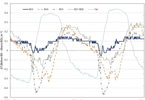
The spatial and temporal temperature differences observed between individual beaver dams from a 2-day period show that each dam influences the system differently throughout each day (Fig. 9). A comparison of absolute temperatures above and below individual beaver dams, where a positive change represents net warming and negative change repre-sents net cooling below the beaver dam, illustrates a gen-eral downstream warming trend which cumulatively propa-gated downstream below beaver dam 8 (Fig. S3). Although the temperature increase for each dam was generally within the accuracy of the temperature sensor (±0.2◦C), the cu-mulative impact of multiple dams showed more significant downstream warming.
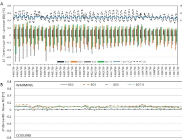
Based on the data shown within Fig. 10, daily ranges (daily maximum minus daily minimum values) of temperature dif-ferences below and above each beaver dam (1T) provide ad-ditional information regarding the spatial variability among individual dams within each day (Fig. 10a). However, when looking at 24 h moving averages (Fig. 10b),1T values fall within the accuracy of the sensors and highlight the impor-tance of the temporal scale (frequency) of measurements when determining the impacts of beaver dams on stream sys-tems.
4 Discussion
[image:9.612.46.289.65.304.2]Figure 6. Change in discharge (1Q) and temperature (1T) over the study reach from 2008 to 2010. This 5-day period in July illustrates variability over shorter temporal scales. The %1Qand %1T are relative to the discharge and temperature at the upstream inflow location (PT515). The %1Qwere averaged over a 1 h interval, while the %1T represents 5 min temperature values.
Table 4. Sub-reach-scale mean residence times for 2008 and 2010.
2008 2010
Sub-reach Stream distance Stream length Mean residence time Beaver dam Mean residence time
(m) (m) (min) (min)
2 692–877 185 8 3, 4 36
3 877–995 118 4 5
4 995–1087 92 4.5 5 15
5 1087–1235 148 6.5 7, 8 29
6 1235–1291 56 4 4
Total (min) 27 89
temporal scales (instantaneous to continuous over a period of years) to draw meaningful conclusions (Kemp et al., 2012; Gibson and Olden, 2014). Furthermore, the results are often inappropriately generalized beyond the scales of the obser-vations. Our observations provide an opportunity to quantify the influences of beaver dams on stream flow and tempera-tures, while demonstrating how beaver dams impact stream hydrologic and temperature regimes at different spatial and temporal scales.
The reach-scale results of our study suggest an overall in-crease in1Qfrom 2008 to 2010 based on changes in flow conditions due to beaver dam building activity (Fig. 2). The increases in gains during the spring can be attributed to sur-face and subsursur-face lateral inflows. However, the impacts of the beaver dams are more apparent during low-flow con-ditions when the study reach slowly transitions from los-ing in 2008 to gainlos-ing in 2010 (Fig. 3). As the number of
[image:10.612.92.506.363.488.2]communica-Figure 7. Groundwater elevations grouped by individual
sub-reaches and shown with channel water surface elevations. The groundwater elevations were measured 4 times in 2008, 5 times in 2009, and 4 times in 2011. The water surface elevation in the chan-nel represents the average yearly value for each sub-reach. There is a gradual increase in groundwater elevation and channel water surface elevation in all sub-reaches over the years.
tion, 2013). This suggests that the dominant hydrologic pro-cesses influencing the study reach changed over the period of 3 years as the trend of gaining conditions persisted past the irrigation season (Fig. 3). Groundwater elevations further illustrate the changes relative to channel surface water ele-vations over time. Although there is a potential for different flow paths in our study reach and head gradients do not nec-essarily translate into fluxes, there were notable increases in the groundwater table (Fig. 7). These changes were likely due to increased water surface elevations in the beaver ponds for consecutive years. The localized increases in groundwa-ter elevations are further elevated each spring due to high flows, inundation of the flood plain, and general high surface water elevations throughout the reach. As the flow and sur-face water elevations drop throughout each summer, there are positive groundwater gradients towards the stream through-out this season and, therefore, the reach gains water. To pro-vide a comparison, we can use baseline1Qand %1Qfrom the control reach just upstream for the same 3-year period (Table 3). These data show that the control reach was losing water for all 3 years except for summer of 2008. In contrast to the beaver impacted study reach, the losing trend in the control reach is more pronounced with each year and it is at its maximum in 2010.
When considering the smaller spatial scales (sub-reach, beaver dam) there is great variability in terms of losses and gains that are not fully understood from the reach-scale ob-servations in the study reach with beaver dams (Figs. 7, 8, Table 4). This variability is due to many different mech-anisms occurring in and around beaver dams, including groundwater–surface water exchanges (Lautz and Siegel, 2006; Janzen and Westbrook, 2011). However, the sub-reach-scale variability in this study (Fig. 8) was primarily due to high crest dams forcing year round overbank flow. Much of the overbank flow was either returned to the main
chan-Figure 8. Sub-reach stream discharge (Q) estimates for 2008 and 2010 representing longitudinal flow variability before and after beaver colonization. %1Qis calculated from flow at the end of the sub-reach minus the flow at the beginning of the sub-reach relative to the upstream value.
nel through side channels or was diverted to the off-channel beaver ponds. These changes in flow paths influenced the mass recovery in our tracer study in 2010 and the highest mass loss occurred in sub-reaches with big beaver dams and multiple side channels. Furthermore, the window of detec-tion inherent to tracer experiments (i.e., the elapsed time over which the tracer is observed) varies as a function of stream characteristics, such as transient storage volume, and stream velocity and discharge (Harvey and Wagner, 2000). In turn, any tracer mass not recovered within the window of detection will be considered a permanent loss even if some mass even-tually returns to the stream (e.g., Ward et al., 2013). Because the changes to the study reach between years influenced the window of detection and, therefore, the reported mass recov-eries, our conclusions are primarily based on the net changes to flow (%1Q) that are less sensitive to a changing window of detection.
[image:11.612.314.543.65.325.2] [image:11.612.48.290.67.185.2]Figure 9. Spatial variability in stream temperature throughout
indi-vidual beaver dams (BD). Temperature differences (1T) were cal-culated based on 10 min temperature records from locations down-stream and updown-stream of the beaver dam and pond. These data il-lustrate that there is a time lag between air temperature and stream temperature and that there can be measurable differences in temper-atures at the beaver dam spatial scale that vary diurnally. It further shows the variability in temperature differences between the dams.
the study period (Fig. 7). These differing results from dilu-tion gaging and groundwater levels highlight the importance of temporal scales and repeated measurements considered in this present work. They also indicate that without this con-sideration, the differences between measurement techniques can lead to contradicting conclusions as discussed within Schmadel et al. (2014). It is also important to note that the positive head gradients on river left (in a downstream direc-tion) illustrate why sub-reach 5 is gaining water (Figs. 7; S2). However, it is also likely losing water on river right. Sub-reach 6 is gaining water due to both the main and side chan-nels meeting again (Figs. 1, 8).
Our temperature results demonstrate the considerable spa-tial and temporal variability in stream temperature caused by beaver dams. We captured the warming effect at the reach scale over a period of 3 years (Figs. 4, 5). However, the data at this scale do not portray the thermal heterogeneity illus-trated by the beaver dam scale temperatures (Figs. 9, 10). Similarly, the temporal scale is of importance when deter-mining impacts of beaver dams. For example, the 5 min tem-perature data captured temtem-perature fluctuations during the day that may play an important role in fish habitat manage-ment and restoration (Fig. 6c–d). This daily variability would not be captured if only daily averages or instantaneous mea-surements were recorded. The lag times in peak temperatures from 2008 to 2010 (more apparent at shorter temporal scales (e.g., Fig. S4)) are likely due to different flow conditions, air temperatures, solar radiation, precipitation, and channel mor-phology.
To understand the significance of simultaneously consider-ing the spatial and temporal scale of measurements, Figs. 9–
10 illustrate the temperature variability for five beaver dams while providing a comparison between the dams. Individual beaver dams introduce more variability than that observed at the reach scale with warming and/or cooling effects dur-ing different times of the day. These individual responses are likely due to the diverse beaver dam morphology, size of the beaver dam, and size of the beaver pond (Fuller and Peckarsky, 2011; McGraw, 1987). However, considering a longer temporal scale, the temperature variability associated with a 24 h moving average falls within a measurement error (±0.2◦C) (Fig. 10b).
With the transition from a losing to gaining reach, one might expect a decrease in temperature during the summer due to the addition of colder groundwater. However, we observed increased warming over the study reach. Based on this expectation that a gaining reach should be cool-ing, it is important to discuss the different heat transfer mechanisms influencing instream temperature responses. It is well established that surface heat fluxes (shortwave radi-ation, incoming and outgoing long-wave radiradi-ation, conduc-tion/convection, and evaporation/condensation) and subsur-face processes (e.g., bed conduction, groundwater/hyporheic exchanges) are often the primary factors dictating stream temperature responses (e.g., Cardenas et al., 2014; Evans et al., 1998; Moore et al., 2005; Neilson et al., 2010a, b; Sinokrot and Stefan, 1993; Webb and Zhang, 1997; Westhoff et al., 2007; Younus et al., 2000). When considering the tran-sition between pre- and post-beaver colonization, the dou-bling of the channel surface area is critical because surface heat fluxes are scaled with the area (Neilson et al., 2010a). The influence of these fluxes on temperature is also depen-dent on the difference in the volume of water in the channel and the residence time within the study reach. Based on the observed temperature increases, the doubling of the surface area (Fig. 1; Table 3) and the tripling of the residence time (Table 4) negate the buffering effects of an almost quadrupled main channel water volume (Table 3) and the cooling effects associated with groundwater inflows. As found within other prior studies, the general downstream warming is due pri-marily to influences of solar radiation (Cook, 1940; Evans et al., 1998; Johnson, 2004; Webb and Zhang, 1997).
spa-Figure 10. (a) Daily range of temperature differences (1T )(downstream temperature minus upstream temperature) of each beaver dam (BD) based on 10 min temperature records. Beaver dams 7 and 8 were considered to be one complex. The air temperature (blue line) and stream temperature at the inflow (PT515, black-dashed line) illustrate the diurnal patterns; (b) 24 h moving average of1T.
tial scales (e.g., sub-reach, beaver dam, and even microhab-itat units) are key for understanding the influences on the aquatic ecosystem (e.g., Billman et al., 2013; Westbrook et al., 2011). Spatial heterogeneity (patchiness) and spatial pat-terns in heterogeneity change with spatial scale (Cooper et al., 1997). Since most of the ecological interactions in het-erogeneous streams happen in conditions that are different from mean conditions, they cannot be captured with point measurements, or with models that focus on understand-ing average conditions (Brentnall et al., 2003; Grünbaum, 2012). This highlights the need to concentrate on variables and processes that capture spatial patchiness at different spa-tial scales in stream ecosystems.
This study emphasizes the need to understand the variabil-ity in flow and temperatures at different spatial and temporal scales. Furthermore, these data begin to provide an expla-nation as to why the current literature provides inconsistent information regarding the influences of beaver colonization. Although it is difficult to make any generalizations about the hydrologic and thermal impacts of beaver dams (e.g., beaver dams increase temperature), we measured an increased vari-ability in flow and temperature that have been qualitatively discussed in previous studies. Our quantification of the vari-ability across different spatial and temporal scales provides a context for better interpreting the inconsistent information found in the literature. In a given locality or under specific
circumstances, we contend that the patterns of increasing variability in flows and temperatures should create and main-tain more heterogeneous habitat that has a greater probability of providing multiple niches and supporting greater biodi-versity. We believe that this observed hydrologic and thermal variability is an important and more generalizable attribute of beaver dams. Variability in temperature, flow properties, and the associated increase in microhabitat complexity are often restoration goals. However, if beaver are being considered as a restoration tool (e.g., Utah Beaver Management Plan), the importance of further understanding and predicting their impacts on stream systems at different spatial and temporal scales is a necessity. Based on these findings, future efforts in understanding the impacts of beaver dams on hydrologic and temperature regimes should begin by identifying the spatial and temporal scales of data required to address specific ques-tions and/or restoration goals. Ultimately, more quantitative field and modeling studies are needed to fully understand im-pacts of beaver on stream ecosystems for the potential use of beaver as a restoration tool.
5 Conclusion
[image:13.612.116.481.65.346.2]of understanding the spatial and temporal scales of those im-pacts. Based on the flow and temperature data collected over the period of pre- and post-beaver colonization, we found a general increase in stream discharge and stream tempera-tures at the reach scale. The reach transitioned from slightly losing in 2008 (pre-beaver colonization period) to gaining in 2010 (post-beaver, second year into beaver colonization). Similarly, we observed a downstream warming effect over the 3-year study period. We found that the reach-scale hy-drologic and temperature changes do not reflect the variabil-ity captured at smaller sub-reach and beaver dam scales. For example, temperature measurements at finer temporal scales (5–10 min records throughout each day) revealed significant within-day variability at smaller spatial scales that was not captured at the reach scale. Our most important and likely transferable findings are with regards to the increase in hy-drologic and thermal variability that beaver dams produce. We captured natural variability of hydrologic and thermal processes at the sub-reach scale prior to beaver dam influ-ences and show how this variability increased after beaver colonization. While some sub-reaches showed gaining trends from 2008 to 2010, some began losing due to flow being rerouted by dam construction. In addition, daily stream tem-perature variability increased from 2008 to 2010. Further-more, these data illustrate the influence of individual beaver dams that can cumulatively contribute to the downstream warming and/or cooling. Such hydrologic and temperature variability would be lost if only reach-scale measurements were collected. In the context of ecosystem impacts and po-tentially using beaver as a restoration tool, where habitat heterogeneity and increased system resilience is achieved through higher rates of biodiversity, we argue that quantify-ing the range and increase in variability may be far more im-portant than measuring a minor and often inconsistent change in mean conditions.
The Supplement related to this article is available online at doi:10.5194/hess-19-3541-2015-supplement.
Acknowledgements. This research was primarily funded by the
Utah Water Research Laboratory and partially supported by Na-tional Science Foundation EPSCoR grant IIA 1208732 awarded to Utah State University as part of the State of Utah EPSCoR Re-search Infrastructure Improvement Award. Any opinions, findings, and conclusions or recommendations expressed are those of the au-thors and do not necessarily reflect the views of the National Sci-ence Foundation. The authors would like to thank the Utah Division of Wildlife Resources for facilitating this research and the numer-ous field crew members for their help with data collection. In ad-dition, the authors would like to thank to Megan Klaar, Michael Pollock, and an anonymous reviewer for their thoughtful comments that greatly improved this manuscript.
Edited by: F. Pappenberger
References
Albert, S. and Trimble, T.: Beavers are partners in riparian restora-tion on the Zuni Indian Reservarestora-tion, Ecological Restorarestora-tion, 18, 87–92, doi:10.3368/er.18.2.87, 2000.
Andersen, D. C., Shafroth, P. B., Pritekel, C. M., and O’Neill, M. W.: Managed flood effects on beaver pond habitat in a desert riverine ecosystem, Bill Williams River, Arizona USA, Wetlands, 31, 195–206, doi:10.1007/s13157-011-0154-y, 2011.
Barrett, K. R.: Ecological Engineering in Water Resources, Water Int., 24, 182–188, doi:10.1080/02508069908692160, 1999. Beschta, L. R., Bilby, E. R., Brown, W. G., Holtby, L. B., and
Hofs-tra, D. T.: Stream temperature and aquatic habitat: fishersies and forestry interactions, in: Streamside Management: Forestry and Fishery Interactions, edited by: Salo, E. O. and Cundy, T. W., University of Washington, Institute of Forest Resources, Seattle, WA, Contribution No. 57, 191–232, 1987.
Billman, E., Kreitzer, J., Creighton, J. C., Habit, E., McMillan, B., and Belk, M.: Habitat enhancement and native fish conservation: can enhancement of channel complexity promote the coexistence of native and introduced fishes?, Environ. Biol. Fish., 96, 555– 566, doi:10.1007/s10641-012-0041-2, 2013.
Brentnall, S. J., Richards, K. J., Brindley, J., and Murphy, E.: ton patchiness and its effect on larger-scale productivity, J. Plank-ton Res., 25, 121–140, doi:10.1093/plankt/25.2.121, 2003. Briggs, M. A., Lautz, L. K., and McKenzie, J. M.: A comparison of
fibre-optic distributed temperature sensing to traditional methods of evaluating groundwater inflow to streams, Hydrol. Process., 26, 1277–1290, doi:10.1002/Hyp.8200, 2012.
Burns, D. A. and McDonnell, J. J.: Effects of a beaver pond on runoff processes: comparison of two headwater catchments, J. Hydrol., 205, 248–264, doi:10.1016/S0022-1694(98)00081-X, 1998.
Cardenas, M. B., Doering, M., Rivas, D. S., Galdeano, C., Neil-son, B. T., and RobinNeil-son, C. T.: Analysis of the temperature dynamics of a proglacial river using time-lapse thermal imag-ing and energy balance modelimag-ing, J. Hydrol., 519, 1963–1973, doi:10.1016/j.jhydrol.2014.09.079, 2014.
Cey, E. E., Rudolph, D. L., Parkin, G. W., and Aravena, R.: Quanti-fying groundwater discharge to a small perennial stream in south-ern Ontario, Canada, J. Hydrol., 210, 21–37, doi:10.1016/S0022-1694(98)00172-3, 1998.
Cook, D. B.: Beaver–trout relations, J. Mammal., 21, 397–401, doi:10.2307/1374874, 1940.
Cooper, S. D., Barmuta, L., Sarnelle, O., Kratz, K., and Diehl, S.: Quantifying spatial heterogeneity in streams, J. N. Am. Benthol. Soc., 16, 174–188, 1997.
Evans, E., McGregor, G. R., and Petts, G. E.: River energy budgets with special reference to river bed processes, Hydrol. Process., 12, 575–595, 1998.
Fanelli, R. M. and Lautz, L. K.: Patterns of water, heat, and solute flux through streambeds around small dams, Ground Water, 46, 671–687, doi:10.1111/j.1745-6584.2008.00461.x, 2008. Fuller, M. R. and Peckarsky, B. L.: Ecosystem engineering by
Gibson, P. P. and Olden, J. D.: Ecology, management, and conservation implications of North American beaver (Castor
canadensis) in dryland streams, Aquat. Conserv., 24, 391–409,
doi:10.1002/aqc.2432, 2014.
Gooseff, M. N. and McGlynn, B. L.: A stream tracer technique em-ploying ionic tracers and specific conductance data applied to the Maimai catchment, New Zealand, Hydrol. Process., 19, 2491– 2506, doi:10.1002/hyp.5685, 2005.
Grünbaum, D.: The logic of ecological patchiness, Interface Focus, 2, 150–155, doi:10.1098/rsfs.2011.0084, 2012.
Gurnell, A. M.: The hydrogeomorphological effects of beaver dam-building activity, Prog. Phys. Geog., 22, 167–189, 1998. Harvey, J. W. and Wagner, B. J.: 1 – Quantifying hydrologic
interac-tions between streams and their subsurface hyporheic zones, in: Streams and Ground Waters, edited by: Jones, J. B. and Mulhol-land, P. J., Academic Press, San Diego, California, A volume in Aquatic Ecology, 3–44, doi:10.1016/B978-012389845-6/50002-8, 2000.
Hill, A. R. and Duval, T. P.: Beaver dams along an agricultural stream in southern Ontario, Canada: their impact on riparian zone hydrology and nitrogen chemistry, Hydrol. Process., 23, 1324– 1336, doi:10.1002/Hyp.7249, 2009.
Janzen, K. and Westbrook, C. J.: Hyporheic flows along a chan-nelled peatland: influence of beaver dams, Can. Water Resour. J., 36, 331–347, doi:10.4296/cwrj3604846, 2011.
Johnson, S. L.: Factors influencing stream temperatures in small streams: substrate effects and a shading experiment, Can. J. Fish. Aquat. Sci., 61, 913–923, 2004.
Kemp, P. S., Worthington, T. A., Langford, T. E. L., Tree, A. R. J., and Gaywood, M. J.: Qualitative and quantitative effects of reintroduced beavers on stream fish, Fish Fish., 13, 158–181, doi:10.1111/j.1467-2979.2011.00421.x, 2012.
Kilpatrick, A. F. and Cobb, D. E.: Measurement of Discharge Using Tracers, Techniques of Water-Resources Investigations, Book 3, Chapter A16, 52 pp., US Geological Survey, Alexandria, VA, 1985.
Lautz, L. K. and Siegel, D. I.: Modeling surface and ground water mixing in the hyporheic zone using MOD-FLOW and MT3D, Adv. Water Resour., 29, 1618–1633, doi:10.1016/j.advwatres.2005.12.003, 2006.
Margolis, B. E., Castro, M. S., and Raesly, R. L.: The impact of beaver impoundments on the water chemistry of two Ap-palachian streams, Can. J. Fish. Aquat. Sci., 58, 2271–2283, doi:10.1139/cjfas-58-11-2271, 2001.
Merck, M. F. and Neilson, B. T.: Modeling in-pool temperature vari-ability in a beaded arctic stream, Hydrol. Proc., 26, 3921–3933, doi:10.1002/hyp.8419, 2012.
McGraw, M.: Effect of Beaver Dams on Hyporheos Patterns, in: Ecology of streams and rivers, edited by: Hendricks, W., Uni-versity of Michigan, Biological Station, UniUni-versity of Michigan, Ann Harbor, MI, 1987.
McRae, G. and Edwards, C. J.: Thermal characteristics of Wis-consin headwater streams occupied by beaver: implications for Brook Trout Habitat, Trans. Am. Fish. Soc., 123, 641–656, doi:10.1577/1548-8659(1994)123<0641:TCOWHS>2.3.CO;2, 1994.
Meentemeyer, R. K. and Butler, D. R.: Hydrogeomorphic effects of beaver dams in Glacier National Park, Montana, Phys. Geogr., 20, 436–446, doi:10.1080/02723646.1999.10642688, 1999.
Moore, R. D., Sutherland, P., Gomi, T., and Dhakal, A.: Ther-mal regime of a headwater stream within a clear-cut, coastal British Columbia, Canada, Hydrol. Process., 19, 2591–2608, doi:10.1002/hyp.5733, 2005.
Neilson, B. T., Stevens, D. K., Chapra, S. C., and Bandaragoda, C.: Data collection methodology for dynamic tmperature model testing and corroboration, Hydrol. Process., 23, 2902, doi:10.1002/hyp.7381, 2009.
Neilson, B. T., Chapra, S. C., Stevens, D. K., and Bandaragoda, C.: Two-zone transient storage modeling using temperature and so-lute data with multiobjective calibration: 1. Temperature, Water Resour. Res., 46, W12520, doi:10.1029/2009WR008756, 2010a. Neilson, B. T., Stevens, D. K., Chapra, S. C., and Ban-daragoda, C.: Two-zone transient storage modeling using temperature and solute data with multiobjective calibration: 2. Temperature and solute, Water Resour. Res., 46, W12521, doi:10.1029/2009WR008759, 2010b.
Nyssen, J., Pontzeele, J., and Billi, P.: Effect of beaver dams on the hydrology of small mountain streams: example from the Chevral in the Ourthe Orientale Basin, Ardennes, Belgium, J. Hydrol., 402, 92–102, doi:10.1016/j.jhydrol.2011.03.008, 2011. Payn, R. A., Gooseff, M. N., McGlynn, B. L., Bencala, K. E.,
and Wondzell, S. M.: Channel water balance and exchange with subsurface flow along a mountain headwater stream in Montana, United States, Water Resour. Res., 45, W11427, doi:10.1029/2008wr007644, 2009.
Pollock, M. M., Pess, G. R., Beechie, T. J., and Montgomery, D. R.: The importance of beaver ponds to coho salmon production in the Stillaguamish River Basin, Washington, USA, N. Am. J. Fish. Manage., 24, 749–760, doi:10.1577/M03-156.1, 2004.
Pollock, M. M., Beechie, T. J., and Jordan, C. E.: Geomorphic changes upstream of beaver dams in Bridge Creek, an in-cised stream channel in the interior Columbia River Basin, eastern Oregon, Earth Surf. Proc. Land., 32, 1174–1185, doi:10.1002/esp.1553, 2007.
Rantz, S. E.: Measurement and Computation of Streamflow: Com-putation of Discharge, Water Supply Paper, Report 2175, US Ge-ological Survey, Denver, 2, 285–631, 1982.
Rosell, F., Bozsér, O., Collen, P., and Parker, H.: Ecological im-pact of beavers Castor fiber and Castor canadensis and their ability to modify ecosystems, Mammal Rev., 35, 248–276, doi:10.1111/j.1365-2907.2005.00067.x, 2005.
Salyer, J. C.: Preliminary report on the beaver-trout investigation, American Game, 24, 6–15, 1935.
Schmadel, N. M., Neilson, B. T., and Stevens, D. K.: Approaches to estimate uncertainty in longitudinal channel water balances, J. Hydrol., 394, 357–369, doi:10.1016/j.jhydrol.2010.09.011, 2010.
Schmadel, N. M., Neilson, B. T., and Kasahara, T.: Deduc-ing the spatial variability of exchange within a longitudi-nal channel water balance, Hydrol. Process., 28, 3088–3103, doi:10.1002/hyp.9854, 2014.
Shetter, D. S. and Whalls, M. J.: Effect of impoundment on water temperatures of Fuller Creek, Montmorency County, Michigan, J. Wildlife Manage., 19, 47–54, doi:10.2307/3797551, 1955. Shields Jr., F., Cooper, C., and Knight, S.: Experiment in
Sinokrot, B. A. and Stefan, H. G.: Stream temperature dynam-ics: measurements and modeling, Water Resour. Res., 29, 2299– 2312, doi:10.1029/93WR00540, 1993.
Snow, C. J.: Impact of Beaver Ponds on Stream Temperature and on Solar Radiation Penetration in Water, PhD thesis, Utah State University, Logan, Utah, 2014.
Talabere, A. G.: Influence of water temperature and beaver ponds on Lahontan cutthroat trout in a high-desert stream, southeastern Oregon, Oregon State University, Corvallis, OR, 44 leaves, 2002. Ward, A. S., Payn, R. A., Gooseff, M. N., McGlynn, B. L., Bencala, K. E., Kelleher, C. A., Wondezell, S. M., and Wagener, T.: Vari-ations in surface water-ground water interactions along a head-water mountain stream: Comparison between transient storage and water balance analyses, Water Resour. Res., 49, 3359–3374, doi:10.1002/wrcr.20148, 2013.
Webb, B. and Zhang, Y.: Spatial and seasonal variability in the com-ponents of the river heat budget, Hydrol. Process., 11, 79–101, 1997.
Westbrook, C. J., Cooper, D. J., and Baker, B. W.: Beaver as-sisted river valley formation, River Res. Appl., 27, 247–256, doi:10.1002/Rra.1359, 2011.
Westhoff, M. C., Savenije, H. H. G., Luxemburg, W. M. J ., Stelling, G. S., van de Giesen, N. C., Selker, J. S., Pfister, L., and Uh-lenbrook, S.: A distributed stream temperature model using high resolution temperature observations, Hydrol. Earth Syst. Sci., 11, 1469–1480, doi:10.5194/hess-11-1469-2007, 2007.
White, D. S.: Biological relationships to convective flow pat-terns within stream beds, Hydrobiologia, 196, 149–158, doi:10.1007/Bf00006106, 1990.
Younus, M., Hondzo, M., and Engel, B.: Stream temperature dy-namics in upland agricultural watersheds, J. Environ. Eng., 126, 518–526, 2000.
Zellweger, G. W.: Testing and comparison of four ionic tracers to measure stream flow loss by multiple tracer injection, Hydrol. Process., 8, 155–165, doi:10.1002/hyp.3360080206, 1994. Utah Division of Wildlife Resources: Utah Beaver Management