Analysis of Support Vector Regression Model for Micrometeorological Data Prediction

(1)

Analysis of Support Vector Regression Model for

Micrometeorological Data Prediction

Yuya Suzuki

1

_{, Yukimasa Kaneda}

2

_{, Hiroshi Mineno}

1,*

1_{Graduate School of Informatics, Shizuoka University, Japan} 2_{Faculty of Informatics, Shizuoka University, Japan}

Abstract

This paper aims to reveal the appropriate amount of training data for accurately and quickly building a support vector regression (SVR) model for micrometeorological data prediction. SVR is derived from statistical learning theory and can be used to predict a quantity in the future based on training that uses past data. Although SVR is superior to traditional learning algorithms such as the artificial neural network (ANN), it is difficult to choose the most suitable amount of training data to build the appropriate SVR model for micrometeorological data prediction. The challenge of this paper is to reveal the periodic characteristics of micrometeorological data in Japan and determine the appropriate amount of training data to build the SVR model. By selecting the appropriate amount of training data, it is possible to improve both prediction accuracy and calculation time. When predicting air temperature in Sapporo, the prediction error was reduced by 0.1°C and the calculation time was reduced by 98.7% using the appropriate amount of training data.

Keywords

Support Vector Regression (SVR),

Micrometeorological Data Prediction, Agricultural Support Systems

1. Introduction

Some kinds of sensor network-based agricultural support systems that enable users to monitor and control the environment in greenhouse horticulture or fields have been studied and developed [1-6]. It is difficult for farmers to decide and set the control parameters properly and control equipment based on priority and symptom diagnosis to cultivate high-quality plants and also set the state of these plants in a changing environment. Although model predictive control (MPC) in industry is an effective means to deal with multivariable constrained control problems, a key issue for controlling the environment appropriately is how to develop a precise prediction model for micrometeorological data. Micrometeorological data is defined as meteorological data that is affected by the surface of the earth, for example,

air temperature, relative humidity, amount of CO2, and soil moisture.

Classical statistical procedures as well as artificial neural networks (ANNs) have already been applied for predicting micrometeorological data [7-14]. ANNs are useful alternatives to traditional statistical modeling in many scientific disciplines. They are composed of a large number of possible non-linear functions, or neurons, each with several parameters that are fitted to data through a computationally intensive training process. Although ANNs are effective for non-linear regression, they also have some drawbacks. The algorithms cannot avoid becoming stuck in a local optimum, which can lead to a sub-optimal solution [15]. Besides, it is difficult to obtain the structure of a network in advance. Therefore, the network has to be optimized by considering, for example, how many neurons and hidden layers would be necessary, what kind of activation functions would be appropriate, and how to connect the neurons with each other to form a network.

Another alternative learning method that has been applied for time series prediction is support vector regression (SVR). The SVR algorithm is an extension of the popular classification method, the support vector machine (SVM). The basic idea is to adjust the possible hypotheses with linear regression by considering the width of the margin of the regression plane. By applying implicit mapping via a kernel function, SVR redefines the dot product in the linear regression method. We need to choose a proper kernel function from a small set and maintain some additional parameters for the chosen kernel function. Although several papers suggest that SVR performs well in many time series prediction problems [16-20], it is difficult to choose the most suitable amount of training data to build the SVR model for micrometeorological data prediction.

The aim of this paper is to reveal the appropriate amount of training data for accurately and quickly building an SVR model for micrometeorological data prediction. Furthermore, this paper shows that it is possible to improve both the prediction accuracy and the calculation time by choosing the appropriate training period.

(2)

Section II showsrelated work in micrometeorological data prediction. Section III shows the experimental environment that reveals the periodic characteristics of micrometeorological data and the appropriate amount of training data to build the SVR model. Section IV shows the results of the evaluation experiment, and Section V shows the conclusion and future work.

2. Related Work

2.1. Overview

Researchers have investigated accurate environmental prediction using, for example, ANNs and SVR. The ANN is a popular data modeling algorithm that mimics the operation of neurons in the human brain. It is used to express complex functions that conduct nonlinear mapping from

_ℜ

J_to

_ℜ

k_,

where J and K are the dimensions of the input and output space, respectively [21].

The SVR algorithm is an extension of the popular classification algorithm, the support vector machine (SVM) [22-26]. The SVM is a machine learning algorithm developed by Vapnik and his co-workers [27]. In the SVM’s original form, the SVM was designed to be used as a classification tool. On its introduction, researchers applied it to classification problems such as optical character recognition and face detection [28-31]. Subsequently, this algorithm was extended to the case of regression or estimation and termed SVR.

The SVM avoids the local extreme value problem that occurs in the ANN. The SVM replaces traditional empirical risk with structure risk minimization and solves the quadratic optimization problem that can theoretically obtain the global optimal solution [17].

2.2. Artificial Neural Network

ANN models have been used for air prediction [9-14]. Kadu et al. [9] implemented air prediction in a project where they used Statistica software to provide the Statistica artificial neural network (SANN) (which was used here for air temperature prediction) and heavy weather software (which was used for data gathering). As a result, the ensemble networks could be trained effectively without excessively compromising the performance. The ensemble networks could achieve good learning performance because one of the ensemble’s members was able to learn from the correct learning pattern even though the patterns were statistically mixed with erroneous learning patterns.

The original ANN air temperature models of Jain et al. [11] were developed using NeuroShell [22]. This method was limited to 32,000 training patterns due to software constraints. Smith et al. [13] overcame this limitation by implementing a custom ANN suite in Java. In addition, several enhancements were made to the original approach, which included the addition of seasonal variables, extended duration of prior variables, and use of multiple instantiations for parameter selection.

2.3. Support Vector Regression

SVR models have also been used for various weather predictions [16-20]. Liu et al. [17] proposed the new wavelet-SVM model that can obtain more detailed information contained in the time series process and produce better prediction results. Therefore, it is not rigorous to predict a future trend using SVM regression in these processes. Regression on wavelet coefficients based on SVM on different scales on a time series that fully considers the impact of regularity for the time series on various scales and at various frequencies has been presented. The problem that was caused by continuous wavelet transform in the discrete time series has been solved through wavelet transform. This result indicates that the prediction accuracy of the SVM method based on wavelet transform is significantly higher than that based on SVM and neural network' back propagation (BP) models. Chevalier et al. [18] built an SVR short-term air temperature prediction model and proposed a method for reducing training data. This method offers a quick means of producing reduced training data from a large amount of training data. It works by repeatedly and randomly sampling from the complete training set. Candidate training sets are quickly evaluated by applying the SVR algorithm with relaxed parameter settings, which reduces training time. The more time-consuming SVR experiments are only performed after an appropriate reduced set has been produced. Even with computational limitations on the number of training patterns that the SVR algorithm was able to handle, it produced results that were comparable to and in some cases more accurate than those obtained with ANNs. Mori et al. [19] predicted the daily maximum air temperature. This method used SVR and reduced the average prediction error of the next day's maximum air temperature by 0.8% compared to that of the ANN.

3. Experimental Environment

3.1. Basic Theory of Support Vector Regression

Suppose that SVR is given training data

⊂

)}

,

(

),...,

,

{(

x

1

y

1

x

k

y

k X×ℜ, where

X

means the space

of the input patterns

(

_e

.

_g

.

_X

₌

_ℜ

d

)

_{. For example, these} might be exchange rates for a currency measured for subsequent days together with corresponding econometric indicators. In the case of ε-SVR, which is a typical SVR method, the goal is to ﬁnd the function

f

(

x

)

that has at most ε deviation from the actually obtained targets

y

_i for all the training data and at the same time is as ﬂat as possible. In other words, ε-SVR does not take errors into account as long as they are less than ε; ε-SVR will not accept any deviation larger than this. To explain the theory of SVR simply, a linear function

f

is used:

.

,

)

(

x

=

w

x

+

b

with

w

∈

X

b

∈

ℜ

(3)

where

⋅

,

⋅

means the dot production in

X

. Flatness in the case of expression (1) means that one is seeking a small

w

. One way to ensure this is to minimize the norm, i.e.

w

2

=

,

. Thus, this minimization problem can be expressed as a convex optimization problem:

   ≤ − + ≤ − − . , , to subject 2 1 minimize 2

e

i i i i y b x w b x w y w (2)

This expression assumes that such a function

f

actually exists that approximates all pairs

(

x

_i

,

y

_i

)

with

e

precision. In other words, the convex optimization problem is feasible. However, it does not support this case, and ε-SVR may be necessary to allow for some errors. Analogously, the “soft margin” loss function [7], which was adapted for SVM, can be used to introduce slack variables

ξ

_i and

ξ

_i*to cope with otherwise infeasible constraints of the optimization problem (2). Hence, it is expressed in expression (3).

(

)











≥

+

≤

−

+

≤

−

+

∑

=

.

0 ,

,

to

subject

2

1 minimize

* * 1 * 2 i i i i i i i i l

i i i

y

b

x

w

b

x

w

y

C

w

ξ

e

ξ

e

ξ

(3)

The constant

C

>

0

determines the trade-off between the fitness of f and the amount up to which deviations larger than

e

are tolerated. This corresponds to dealing with the so-called

e

−

Insensitive loss function

ξ

_e described by

   − ≤ = . 0 : otherwise if e ξ e ξ

ξ_e (4)

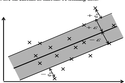
Figure 1 shows this situation. Only the points outside the shaded region contributed to the cost to the extent that the deviations were penalized in a linear fashion. It turns out that in most cases the optimization problem (3) could be solved more easily in its dual formulation.

To solve this problem, Lagrange multipliers were used [8]. Hence, the local solution obtained by Lagrange multipliers was always the global solution. Accordingly, SVR is superior to traditional learning algorithms, such as ANNs, that might fall into a local solution. On the other hand, SVR has the fault that the calculation time increases logarithmically when the quantity of learning data increases. Thus, to avoid increasing the calculation time, you should

[image:3.595.321.538.85.230.2]

not use an enormous amount of training data.

Figure 1. Soft margin loss setting for linear SVM

3.2. Assumed Environment

To analyze the periodic characteristics of micrometeorological data in Japan and determine the appropriate amount of training data needed to build the SVR model, we hypothesize that the characteristics of micrometeorological data change in accordance with time because of four seasons, rainy season, and dry season. In our experiment, we used the micrometeorological data of Japan for the past three years and for four areas where climate conditions are different.

In the experiment, we used the open micrometeorological data of Japan that was provided by the automated meteorological data acquisition system (AMeDAS). AMeDAS is managed by the meteorological agency in Japan. This system provides micrometeorological data: air temperature, relative humidity, station pressure, precipitation, mean wind, maximum wind, and sunshine duration. The measurement cycle is every ten minutes. Micrometeorological data of four Japanese areas, Sapporo, Tokyo, Hamamatsu, and Naha, were used as evaluation data to be evaluated objectively by using the typical weather characteristics of each different area. Micrometeorological data of the northernmost area (Sapporo), southernmost area (Naha), center area (Hamamatsu), and capital of Japan (Tokyo) were analyzed.

Figure 2 shows the micrometeorological characteristics of the four regions in Japan. Since Japan has four seasons, the characteristics of the climate change depending on the time of year. In addition, the weather characteristics change by region. This figure describes the climatic conditions of each region: maximum air temperature, mean air temperature, minimum air temperature, and precipitation. Sapporo is the coldest region in Japan, and the difference between the high and low air temperatures is large. On the other hand, Naha is the warmest, and the difference is small. The Tokyo and Hamamatsu areas have typical weather characteristics for Japan. Since the micrometeorological data was time series data and the changes in annual climate characteristics were the same, enough evaluations could be obtained by preparing training data for the past three years.

(4)

[image:4.808.68.743.81.403.2]

Figure 2. Meteorological characteristics of four regions

0 100 200 300 400 500 600

-10 0 10 20 30 40

pr

ec

ipi

tat

ion [

m

]

tem

per

at

ur

e [

℃

]

precipitation maximum temperature

mean temperature minimum temperature

0 100 200 300 400 500 600

-10-5 0 5 10 15 20 25 30

pre

ci

pi

ta

tio

n [

mm]

te

mp

era

tu

re

[

℃

]

precipitation maximum temperature mean temperature minimum temperature

0 100 200 300 400 500 600

-10-5 0 5 10 15 20 25 30 35

pre

ci

pi

ta

tio

n [

mm]

te

mp

era

tu

re

[

℃

]

precipitation maximum temperature mean temperature minimum temperature

0 100 200 300 400 500 600

-10 0 10 20 30 40

pr

ec

ipi

tat

ion [

m

]

tem

per

at

ur

e [

℃

]

precipitation maximum temperature

mean temperature minimum temperature

Jan Feb Mar Apr MayJun July Aug Sep Oct Nov Dec Hamamatsu

Jan Feb MarApr May Jun July Aug Sep Oct Nov Dec Sapporo

Jan Feb MarApr May Jun July Aug Sep Oct Nov Dec Tokyo

(5)

The experiments were conducted on the micrometeorological data up to January 2, 2014, and a deficit period was removed from January 1, 2011. A deficit period means the period where a value is partially lost owing to AMeDAS sensor trouble.

3.3. Experiment

In micrometeorological data prediction, it is difficult to model the appropriate SVR model. We think one of the reasons for this is seasonal and secular variation of micrometeorological data. To investigate the transitions of the prediction accuracy of the SVR model depending on the amount of training data, the micrometeorological data for the past three years were divided into 36 months. 36 prediction models were built, and each model’s prediction accuracy was compared.

Micrometeorological data were sorted in ascending order based on time. A row consists of various micrometeorological data, such as air temperature, relative humidity, and dependent variables. Figure 3 shows how the micrometeorological data was divided. Each block represents one month in the past up to January 1, 2014. By dividing the data in this way, a predictive model of every month could be evaluated. It is possible to examine the change in the prediction accuracy in accordance with the amount of training data by evaluating the prediction accuracy of the model, which consisted of the data for each month.

The dependent variables are the air temperature and relative humidity after one hour. The data from January 1, 2011 to January 1, 2014 were used for training data. Meanwhile, the data from January 2, 2014 were used for evaluation data. The SVR model was evaluated by two kinds of experiments: open test and closed test. The open test evaluated the prediction accuracy of the model by using the evaluation data, which is different from the training data used to build the prediction model. Meanwhile, the closed test evaluated the prediction accuracy of the model using

k-fold cross-validation. In this evaluation, micrometeorological data (January 1, 2011 to January 1, 2014) is randomly partitioned into 10 equal-sized sub-data sets. Using k sub-data, sub-data set is used as evaluation data, and the others are used as training data. The closed test repeats 10 times, with each sub-data set used once as the evaluation data. Then, the validation results of each prediction accuracy evaluated k times are averaged, and this value is used as the closed test result. Since the calculation will take a lot of time if the value of k is enlarged, this experiment set the value of k to 10. Both the result of the open test and the closed test were defined by the root mean square error (RMSE) obtained from the difference between the regression curve and the measured curve.

RMSE is expressed in formula (5), where N is the number of test items and

e

_i is the error of the ensemble mean for each test item i averaged over the required spatial region. In addition, the mean of the squared error in formulation (5) is the mean square error (MSE). The RMSE or MSE is the most popular kind of indicator used for evaluating regression models [10, 16-17, 20]. This paper used RMSE as the evaluation indicator.

N

e

RMSE

N

i i

∑

=

1

2

(5)

[image:5.595.103.510.562.749.2]

In this paper, SVR was implemented by LIBSVM [32] for R supported by the e1071 package [33] and Java. It used Rserve [34] for R and the transmission and reception of Java. Rserve is a TCP/IP server that allows other programs to use the facilities of R from various languages without the need to initialize R or link to an R library. Every connection has a separate workspace and working directory. Client side implementations are available for popular languages such as C/C++ and Java. Rserve supports remote connection, authentication, and file transfer.

Figure 3. How meteorological data was divided

Training Data: Meteorological data for past 3 years

(January 1, 2011 – January 1, 2014)

・・・

Past 1 month

Past 2 months

Past 35 months

Past 36 months

1/

2,

2014

Test Data:

Meteorological data in

January2, 2014

1/1, 2014 ~ 12/1, 2013 11/30, 2013

~ 11/1, 2013 1/31, 2011

~ 1/1, 2011

(6)

4. Result and Discussion

4.1. Overview

We evaluated SVR models using the result of the open test and the closed test on the prediction accuracy of one hour later for air temperature and relative humidity. The result of the closed test depended on k-fold cross-validation. Conversely, the result of the open test depended on the difference between the predicted curve and measured curve of January 2, 2014. Since the total amount of data for three years was large (more than 158,000 items), a huge calculation time to tune SVM parameters was required. Thus, this experiment set each parameter (cost parameter C, tube parameter ε, and hyperparameter of RBF γ) to a constant value and tested without parameter tuning using, for example, a grid search. Table 1 shows the SVR parameters.

Table 1. SVR Conditions

Items Contents

Method Epsilon-SVR

Kernel function Radial basis function (RBF)

Cost parameter (C) 1.0

Tube parameter (ε) 0.1

Hyper parameter of RBF(γ₎ _0.2

This experiment was conducted to focus on the change in the prediction accuracy and the change in the dispersion value of the dependent variable. As a result, this experiment showed that there was a relationship between the dispersion value of the dependent variable and the prediction accuracy in air temperature prediction.

[image:6.595.59.299.287.381.2]

4.2. Air Temperature

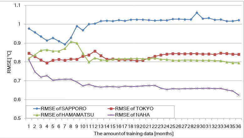
Figure 4 shows the RMSE transitions of the four areas for

air temperature in the open test. It shows that the prediction accuracy of the SVR model that predicts air temperature of Sapporo is the lowest, and that of Naha is the highest. In addition, for the SVR models of Sapporo and Tokyo, prediction models built with all data for the past three years did not have the best prediction accuracy. This experiment revealed that the lowest RMSE of Sapporo was 0.89°C when the model was built using micrometeorological data for the past seven months, and the lowest RMSE of Tokyo was 0.79°C when the model was built using micrometeorological data for the past four months. In addition, although the SVR models that predicted air temperature in Hamamatsu and Naha were based on all data for the past three years and had the lowest RMSE (0.79°C for Hamamatsu and 0.62°C for Naha), it turned out that there was almost no difference in the prediction accuracy of the model based on data that was older than one year. In particular, in Hamamatsu, the difference between the RMSE of models built based on data for the past 11 months and the model based on data for all the past three years is only 0.0048°C.

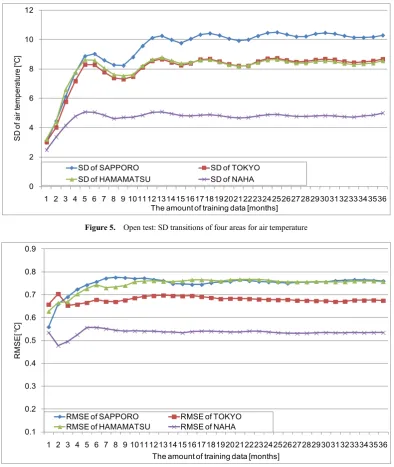
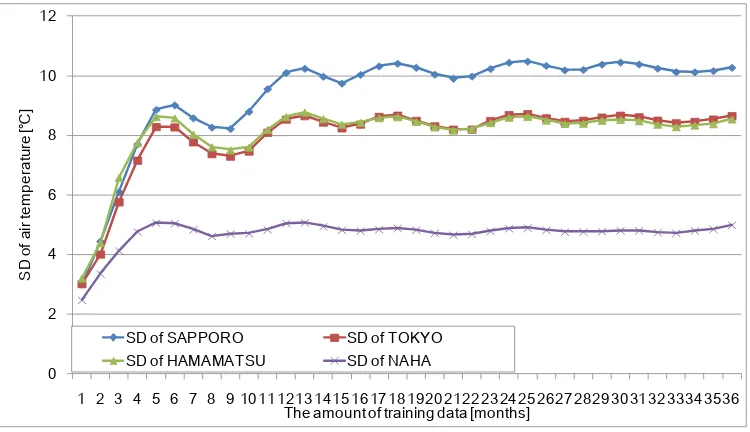
[image:6.595.111.500.513.734.2]

Figure 5 shows the transitions of RMSE and transitions of the standard deviation (SD) of the air temperature in each area. This figure shows that the SD of the air temperature tends to converge in all areas depending on the progress of time. In addition, since the air temperature difference is large, the value for Sapporo is the highest. On the other hand, the value for Naha is the lowest because the air temperature difference is small. When changes of RMSE were observed compared to the characteristic changes of the SD, each graph also shows the convergence of the value of RMSE corresponding to the convergence of the SD. In particular, it shows that three areas other than Naha have distinctive characteristics. The transitions of RMSE in Sapporo, Tokyo, and Hamamatsu hardly changed when the prediction model was built using more than one year of training data.

Figure 4. Open test: RMSE transitions of four areas for air temperature

0.5 0.6 0.7 0.8 0.9 1 1.1

1 2 3 4 5 6 7 8 9 101112131415161718192021222324252627282930313233343536

R

M

SE[

℃

]

The amount of training data [months]

RMSE of SAPPORO RMSE of TOKYO

(7)

[image:7.595.108.503.73.541.2] [image:7.595.109.504.76.283.2]

Figure 5. Open test: SD transitions of four areas for air temperature

Figure 6. Closed test: RMSE transitions of four areas for air temperature

Figures 4 and 5 show that the best performance of the prediction model is not apparent when all the training data is used, and the value of the prediction accuracy converges in accordance with the convergence of SD. The reason is the training data had a different feature that decreased in accordance with the progress of time, and the SVR model did not train new feature values. Thus, it is not necessary for the prediction model to continue training after the dispersion of the air temperature has converged as the calculation time increased.

Figure 6 shows the RMSE transition of the four areas for air temperature in the closed test. The result showed that the prediction accuracy of the model was not improved by increasing the amount of training data as shown by the result of the open test. In particular, the prediction accuracy of the

models tended to be low as the quantity of training data increased. In the case of the models for Sapporo and Hamamatsu, it turned out that the lowest RMSE of Sapporo and Hamamatsu were 0.55°C and 0.62°C, respectively, when models were built using data for the past one month. In addition, the lowest RMSE of Tokyo was 0.65°C when the model was built using data for the past three months; the lowest RMSE of Naha was 0.477°C when the model was built using data for the past two months. The reason there is a difference between the open test result and the closed test result is the open test only evaluated data from January 2, 2014 and the open test result did not assume that there was another period such as the summer duration. However, these results showed the same tendency for magnitude correlation of the prediction accuracy in each area.

0 2 4 6 8 10 12

1 2 3 4 5 6 7 8 9 101112131415161718192021222324252627282930313233343536

SD

of

ai

r t

em

per

at

ur

e [

℃

]

SD of SAPPORO SD of TOKYO

SD of HAMAMATSU SD of NAHA

0.1 0.2 0.3 0.4 0.5 0.6 0.7 0.8 0.9

1 2 3 4 5 6 7 8 9 101112131415161718192021222324252627282930313233343536

R

M

SE[

℃

]

(8)

[image:8.595.119.494.76.292.2]

Figure 7. Closed test: SD transitions of four areas for air temperature

Figure 7 shows the transition of the SD of the four areas for air temperature in the closed test. This shows that the transition of the prediction accuracy of the model tends to converge depending on the convergence of the dispersion of the air temperature like the result of the open test.

These experiments on air temperature prediction revealed that there are two features that affect the prediction accuracy of the model from the result of the open test and the closed test. The first feature is it is not possible to improve the prediction accuracy by increasing the amount of training data in many areas because the data of a different season from the time that air temperature is predicted causes noise, so the weather characteristics change in accordance with seasonal changes.

The second feature is the transition of the prediction accuracy converges in response to the convergence of the air temperature. The air temperature change in Japan is an annual change. Since the data after four seasons has almost the same characteristics as the data before the four seasons, the dispersion of the air temperature tends to converge. Therefore, since past data and characteristics do not change much, it has been suggested that the prediction accuracy of the model will not change much even if the prediction model is trained with new input data. Hence, to select the amount of training data, it is important to determine it before the variance of air temperature converges.

4.3. Relative Humidity

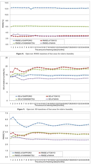
Figure 8 shows the RMSE transitions of the four areas for relative humidity in the open test. It shows that the prediction accuracy of the SVR model predicting the relative humidity of Sapporo is the lowest and the prediction accuracy of the SVR model of Naha is the highest. Meanwhile, the relative humidity prediction model of Tokyo also showed almost the same prediction accuracy as the model of Naha. In addition, in the case of all SVR models that predicted relative humidity, the prediction model built with all data for the past three years did not have the best prediction accuracy. The lowest RMSE of Sapporo was 12.4% when the model was built using the micrometeorological data for the past ten months, and the lowest RMSE of Tokyo was 3.21% when the model was built using data for the past four months. The SVR models of Hamamatsu and Naha had the lowest RMSE (6.54% for Hamamatsu and 3.21% for Naha) when the model was built using micrometeorological data for the past one month. However, unlike the case of air temperature, the increase in the amount of training data did not change the prediction accuracy much.

Figure 9 shows the transitions of SD of the relative humidity in each area. This experiment showed that the transition characteristics of the dispersion values were different depending on the area. As the relative humidity, it fluctuates approximately 50 % a day. On the other hand, the SD of relative humidity only fluctuates by less than 5 %. Thus, it appears that the relative humidity does not change through the year. Therefore, regardless of the amount of training data, regression curves show almost the same value.

0 2 4 6 8 10 12

1 2 3 4 5 6 7 8 9 101112131415161718192021222324252627282930313233343536

SD

of

ai

r t

em

per

at

ur

e [

℃

]

(9)

[image:9.595.119.494.71.741.2]

Figure 8. Open test: RMSE transition of four areas for relative humidity

Figure 9. Open test: SD transitions of four areas for relative humidity

Figure 10. Closed test: RMSE transitions of four areas for relative humidity

0.5 2.5 4.5 6.5 8.5 10.5 12.5 14.5

1 2 3 4 5 6 7 8 9 101112131415161718192021222324252627282930313233343536

R

M

SE[

%

]

RMSE of HAMAMATSU RMSE of NAHA

0 5 10 15 20 25

1 2 3 4 5 6 7 8 9 101112131415161718192021222324252627282930313233343536

SD

of

rel

at

iv

e hum

idi

ty

[%

]

0.5 1.5 2.5 3.5 4.5 5.5 6.5 7.5

1 2 3 4 5 6 7 8 9 101112131415161718192021222324252627282930313233343536

R

M

SE[

%

]

(10)

[image:10.595.115.496.80.513.2] [image:10.595.117.494.299.510.2]

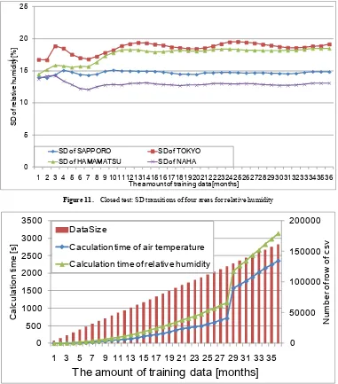
Figure 11. Closed test: SD transitions of four areas for relative humidity

Figure 12. Data size and calculation time every period

Figure 10 shows the RMSE transitions of the four areas in the relative humidity in the closed test. As well as the result of air temperature, the result of the closed test showed that the prediction accuracy of the model was not improved by increasing the amount of training data. In particular, the transition of the prediction accuracy hardly changed the predictive model except for Sapporo. In the case of Sapporo, when the amount of training data was more than eight months, the RMSE converged to approximately 5.5%. In addition, the lowest RMSE of Sapporo was 5.26% when the model was built using data for the past eight months.

The lowest RMSE of Tokyo was 3.89% when the model used data for the past seven months, the lowest RMSE of Hamamatsu was 3.49% when the model used data for the past one month, and the lowest RMSE of Naha was 3.22% when the model used data for the past 35 months. Although Naha's model needed large amounts of data to show the lowest RMSE, there was only a difference of 0.069%

between the RMSE of the model built using data for the past 11 months and the RMSE of the model built using the data for the past 35 months. Therefore, even if it builds a prediction model using a period shorter than 35 months, sufficient predictive accuracy can be maintained. In addition, the reason there is a difference between the result of the open test and the result of the closed test is the same as the reason for the difference for air temperature.

Figure 11 shows the SD transitions of the relative humidity in each area. The figure shows that the transitions of the prediction accuracy of the model tend to converge depending on the convergence of the dispersion of the relative humidity like the result of the open test. Although there was a tendency of the prediction accuracy to converge, generally a change in the prediction accuracy did not result in a big change. Since there was hardly a change in the transition of the prediction accuracy of the relative humidity like the result of the open test, it was difficult to show

0 5 10 15 20 25

1 2 3 4 5 6 7 8 9 101112131415161718192021222324252627282930313233343536

SD

of

rel

at

iv

e hum

idi

ty

[%

]

0 50000 100000 150000 200000

0 500 1000 1500 2000 2500 3000 3500

1 3 5 7 9 11 13 15 17 19 21 23 25 27 29 31 33 35

N

um

ber

of

row

of

c

sv

C

al

cul

at

ion

ti

m

e [

s]

The amount of training data [months]

DataSize

(11)

correlation with the dispersion of the relative humidity.

4.4. Discussion

The computational complexity of SVR is O(n2₎_～_O(n3_).

For SVR in particular, it is important to reduce the amount of training data used for decreasing the calculation time. In many cases, the result of the prediction experiments for air temperature and relative humidity showed that it is better to choose a suitable amount of training data rather than using the data of all parts for 36 months when building an SVR model. Figure 12 shows the transition of the increase in prediction model construction time and the increase of the quantity of training data. It shows that the calculation time for air temperature and relative humidity increased depending on the increase of training data. Thus, it is important to choose the quantity of training data carefully to reduce the calculation time.

For example, in the case of predicting the air temperature for Sapporo on January 2, 2014, it is possible to improve the value of 0.1°C of RMSE by selecting the appropriate amount of training data, which was the past seven months. In addition, the calculation time for building a model using the data for 36 months could be reduced by 98.7%. On the other hand, in the case of predicting the relative humidity for Tokyo on January 2, 2014, the RMSE could be improved by 0.27%, and the calculation time was reduced by 99.3% if the past one month was selected.

In these cases, it is important to select a suitable amount of training data before the convergence of the SD of micrometeorological data occurs. The appropriate period of training data used could be explored by monitoring the change of a differentiation value of the SD. In time series prediction, it is possible to compare a prediction value with a measured value by time course. A prediction value and a measured value are compared sequentially, and if a difference between them exceeds a threshold, we can rebuilds the SVR model at an appropriate time. In addition, it is possible to reduce the total calculation time substantially. As a result, the appropriate amount of training data for accurately and quickly building an SVR model could be determined.

5. Conclusion and Future Work

In this paper, experiments on predicting air temperature and relative humidity revealed the relationship between the prediction accuracy of the model and the amount of training data and showed the appropriate SVR model for each situation. When predicting air temperature, prediction accuracy and calculation time can be improved by determining the quantity of training data in the period before the convergence of SD of air temperature has occurred. In the case of relative humidity, when the data volume was increased per month, there was almost no change in the prediction accuracy. Thus, even if the model is built by using

only the data for the past one month, the model can show enough prediction accuracy though it depends on the assumed application. For example, in the case of predicting the air temperature of Sapporo, it is possible to improve the value by 0.1°C of the RMSE by selecting the appropriate amount of training data. In addition, the calculation time for building a model using the data for 36 months was reduced by 98.7%.

Currently, we are constructing a new machine learning algorithm using the results of this experiment. This experimental result showed that choosing the appropriate data volume out of a vast quantity of training data can improve both prediction accuracy and calculation time. A new machine learning algorithm that can determine a suitable amount of data automatically out of a vast quantity of training data can be built using these results based on detecting the characteristic changes of the SD.

Acknowledgements

This work was partially supported by the budgets for 2013-2014 Strategic Information and Communications R&D Promotion Programme (SCOPE), Ministry of Internal Affairs and Communications, and JSPS Grant-in-Aid for Challenging Exploratory Research (26660198), Japan.

REFERENCES

[1] Kang, B., Park, D., Cho, K., Shin, C., Cho, S., and Park, J. "A study on the greenhouse auto control system based on wireless sensor network," IEEE International Conference on Security Technology (SECTECH), pp.41-44, 2008.

[2] Pierce, F. J., and Elliott T. V. "Regional and on-farm wireless sensor networks for agricultural systems in Eastern Washington," Computers and electronics in agriculture, Vol. 61, pp.32-43, 2008.

[3] Gonda, L., and Cugnasca C. E., "A proposal of greenhouse control using wireless sensor networks," Proceedings of 4th world congress conference on Computers in Agriculture and Natural Resources, 2006.

[4] Ahonen, T., Virrankoski, R., and Elmusrati, M., "Greenhouse monitoring with wireless sensor network," IEEE/ASME International Conference on Mechtronic and Embedded Systems and Applications (MESA), pp.403-408, 2008. [5] Hori, M., Kawashima, E., and Yamazaki, T., "Application of

cloud computing to agriculture and prospects in other fields," Fujitsu Sci, Tech, J. Vol.46, No.4, pp.446-454, 2010. [6] Wang, N., Zhang, N., and Wang, M., "Wireless sensors in

agriculture and food industry -Recent development and future perspective," Computers and electronics in agriculture, Vol.50, pp.1-14, 2006.

(12)

[8] Fletcher, R., "Practical methods of optimization, 2nd ed.," John Wiley & Sons, 2013.

[9] Kadu, P., Wagh, K., and Chatur, P., "Analysis and prediction of air temperature using statistical artificial neural network," IJCSMS, Vol.12, pp.117-122, 2012.

[10] Roebber, P.J., Butt, M.R., Reinke, S.J., and Grafenauer, T.J. "Real-time forecasting of snowfall using a neural network," Weather Forecasting, Vol.22, pp.676-684, 2007.

[11] Jain, A, McClendon, R.W.,, and Hoogenboom, G., "Freeze prediction for specific locations using artificial neural networks," Transactions of the ASABE, Vol.49, Issue.6, pp.1955-1962, 2006.

[12] Smith, B.A., McClendon R.W., and Hoogenboom, G., "Improving air temperature prediction with artificial neural networks," International Journal of Computational Intelligence, Vol.3, Issue.3, pp.179-186, 2006.

[13] Smith, B.A, Hoogenboom, G. and McClendon, R.W. "Artificial neural networks for automated year-round air temperature prediction," Computers and Electronics in Agriculture, Vol.68. Issue.1, pp.52-61, 2009.

[14] Chen, R., and Liu, J., "The area rainfall prediction of up-river valleys in Yangtze River Basin on artificial neural network modes," Scientia Meteorologica Sinica, 24(4), pp.483-486, 2009.

[15] Gori, M. and Tesi, A., "On the problem of local minima in backpropagation," IEEE Transactions on Pattem Analysis and Machine Intelligence, Vol.14, pp.76-86, 1992.

[16] Gill, M.K., Asefa, T., Kemblowski, M.W., and McKee, M., "Soil moisture prediction using support vector machines," Journal of the American Water Resources Association, Vol.42, Issue.4, pp.1033-1046, 2006.

[17] Liu, X., Yuan, S., and Li, L., "Prediction of temperature time series based on wavelet transform and support vector machine," Journal of Computers, Vol.7, pp.1911-1918, 2012. [18] Chevalier, R. F, Hoogenboom, G, McClendon, R. W, and Paz,

J. A, "Support vector regression with reduced training sets for air temperature prediction: a comparison with artificial neural networks," Journal of Neural Computing and Applications, Vol.20, Issue.1, pp.151-159, 2011.

[19] Mori, H., and Kanaoka, D., "Application of support vector regression to temperature forecasting for short-term load forecasting," IEEE International Joint Conference on Neural Networks (IJCNN), 2007.

[20] Hua, X. G, Ni, Y. Q, Ko, J. M, and Wong, K. Y, "Modeling of temperature -frequency correlation using combined principal

component analysis and support vector regression technique," Journal of Computing in Civil Engineering, Vol.21, No.2, pp.122-135, 2007.

[21] Engelbrecht, A.P, "Computational intelligence: an introduction, 2nd Edition," Wiley, 2007.

[22] Frederick, M. D, "Neuroshell 2 user's manual," 1996. [23] Smola, A.J, and Scholkopf, B., "A tutorial on support vector

regression," Statistics and computing, Vol.14, pp.199-222, 2004.

[24] Mattera, D., and Haykin, S., "Support vector machines for dynamic reconstruction of a chaotic system," Advances in kernel methods, MIT Press, pp.211-241, 1999.

[25] Vapnik, V., Golowich, S.E., and Smola, A., "Support vector method for function approximation, regression estimation, and signal processing," Advances in neural information processing systems, Vol.9, pp. 281-287, 1996.

[26] Thissen, U., Brakel, R., Weijer A.P, Melssen, W.J., and Buydens, L.M.C, "Using support vector machines for time series prediction," Chemometrics and intelligent laboratory systems, Vol.69, pp.35-49, 2003.

[27] Cortes, C., and Vapnik, V., "Support-vector networks," Journal of Machine learning, Vol.20(3), pp.273-297, 1995. [28] Osuna, E., Freund, R., and Girosi, F., "Training support

vector machines: an application to face detection," IEEE Computer Society Conference on Computer Vision and Pattern Recognition, 1997.

[29] Ravi, S, and Wilson, S. "Face detection with facial features and gender classification based on support vector machine," IEEE International Conference on Computational Intelligence and Computing Research, 2010.

[30] Scholkopf, B., Burges, C., and Vapnik, V., "Incorporating invariances in support vector learning machines," Artificial Neural Networks (ICANN), LNCS.1112, pp.47-52, 1996. [31] Sun, A., Lim, E., and Liu, Y., "On strategies for imbalanced

text classification using SVM: a comparative study," Decision Support Systems, Vol.48, pp.191-201, 2009. [32] Chang, C.C., and Lin, C.J., "LIBSVM: a library for support

vector machines," ACM Transactions on Intelligent Systems and Technology (TIST), Vol.2, Issue.3, No.27, 2011. [33] Meyer, D., "Support vector machines: The interface to libsvm

in package e1071," 2004.