Modified LLMS Algorithm for Channel Estimation in Noisy Environment

(1)

Modified LLMS Algorithm for Channel Estimation in

Noisy Environment

Dinesh B.Bhoyar

1,*

_{, C.G.Dethe}

2

_{, M.M.Mushrif}

1

1_{Yeshwantrao Chavan College of Engineering, Nagpur, India} 2_{Priyadarshini college of Engineering,Nagpur,India}

*Corresponding Author: [email protected]

Abstract

Intersymbol interference caused by multipath in band limited frequency selective time dispersive channels distorts the transmitted signal, causing bit error at receiver. ISI is the major obstacle to high speed data transmission over wireless channels. Channel estimation is a technique used to combat the intersymbol interference. The objective of this paper is to improve channel estimation accuracy in MIMO-OFDM system by using modified variable step size leaky Least Mean Square (MLLMS) algorithm proposed for MIMO OFDM System. So we are going to analyze Bit Error Rate for different signal to noise ratio, also compare the proposed scheme with standard LMS channel estimation method

Keywords

MIMO, OFDM, MLLMS, ISI

1. Introduction

Due to the development of wireless systems will require a high data rate capable technology. MIMO-OFDM is the best choice for high data rate transmission, because is a widely used modulation and multiplexing technology. In addition improve channel estimation accuracy in MIMO-OFDM system urgent demand. Orthogonal frequency division multiplexing (OFDM)[8] is a widely used modulation and multiplexing technology, which has become the basis of many telecommunications standards including wireless local area networks (LANs), digital terrestrial television (DTT) and digital radio broadcasting. The OFDM divides the available spectrum into a number of overlapping and orthogonal narrowband sub channels. The carriers are made orthogonal to each other by appropriately choosing the frequency spacing between them. The orthogonality will ensure the subcarrier separation at the receiver. It gives better spectral efficiency. It has the advantage of spreading out a frequency selective fade over many symbols. This effectively randomizes burst errors caused by fading or impulse interference. Because of dividing an entire signal bandwidth into many narrow sub bands, the frequency

response over individual sub bands is relatively flat. Multiple Input Multiple Output (MIMO) technology transmit different data streams on different transmit antennas simultaneously. An appropriate processing architecture handles these parallel streams of data. The data rate and the Signal-to-Noise Ratio (SNR) performance can be increased.

Over the year, various computational techniques have been adopted for channel estimation in wireless communication. Least square (LS)[9], Least mean square (LMS),normalized NLMS[15], variable step size LMS(VSS-LMS)[5,16,17] Recursive least square (RLS), Kalman filter, orthogonal Frequency response filtering are some of the well known techniques employed for the purpose of channel estimation[14]more accurately and efficiently. At the same time soft computing approaches such as fuzzy logic, neural network, genetic algorithm and simulated annealing [6] have also been used for channel estimation. However such computing approaches suffer from poor convergence rate and computational complexity is more.

The problem of filter design for estimating the desired signal based on another signal formulated from the deterministic point of view .Channel estimation is usually refers to estimation of the frequency response of the path between the transmitter and receiver, also this is used to optimize performance and maximize the transmission rate [12]. The channel estimation in MIMO-OFDM system is more complicated in comparison with SISO system due to simultaneous transmission of signal from different antennas that cause co-channel interference [13].

(2)

Universal Journal of Communications and Network 1(2): 60-67, 2013 61

efficient and robust with respect to the dynamic variation in the system also the computational complexity of the proposed technique is less as compare to the VLLMS and RLS.MMLLMS gives better performance in the noisy environment.The remainder of the paper is organized as follows. Section 2 represents the system model of MIMO-OFDM system. Section 3 presents the proposed algorithm and formulation of the equations. Section 4 discusses the comparative simulation results of the proposed algorithm with the existing ones. Section 5 concludes the paper.

2. System Model

2.1 MIMO-OFDM System

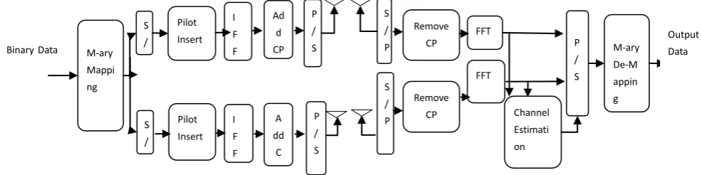
In this paper, we considered MIMO-OFDM system with two transmitting antennas and two receiving antennas. The total number of subcarriers is N. MIMO-OFDM transmitter has parallel transmitter paths which are very similar to the single antenna OFDM system. Each branch performing serial to parallel conversion, pilot insertion, N-point IFFT,

cyclic extension and up-converted to RF before the final data transmission. The channel encoder and the digital modulation can also be done in some spatial modulation system. At the receiver, the cyclic prefix is removed and N-point FFT is performed per received branch. Next, the transmitted symbol per TX antenna is combined and outputted for the subsequent operations like digital demodulation and decoding. Finally all the input binary data are recovered with certain BER [1].Fig.1 shows the MIMO system. The technique develop in this paper can be directly applied to any MIMO-OFDM system. The data block is {b[n,k]:k=0,1---}transmitted into two different signals, {ti[n,k]: k=0,1,...K-1 and i=1,2} at the transmit diversity processor,[2] where, K, k, and i are the number of sub-channels of the OFDM systems, sub-channel index, and antenna index, respectively. This OFDM signal is modulated by using the ti[n,k] where i=1,2. At the receiver, the discrete Fourier transform (DFT or FFT) of the received signal at each receive antenna is the superposition of two distorted transmitted signals. The received signal at the jth_receive

[image:2.595.61.554.355.478.2]

antenna can be expressed as

Figure 1. Block Diagram of MIMO OFDM system

(3)

[ , ] [ , ] [ , ] [ , ]

j ij i j

i

r n k =

∑

w

n k x n k +n n k ₍₁₎

Where, the channel frequency response W n kij[ , ] at

th

k _the

tone of the nthOFDM block, corresponding to the

i

th transmit and jth receive antenna.

n n k

_j

[ , ]

denotes the additive complex Gaussian noise on the

j

th receive antenna and is assumed to be zero mean with variance

σ

2n_.

The noise is uncorrelated for different n’s, k’s or j’s [7]. Above equation can be expressed in matrix form as,

[ ]

1

[ ] n n [ ] [ ]

ij i

n n n

j j j

r

w x

n

=

_∑

+

(2)

[ ]

[ [ , 0], [ ,1],..., [ , 1]]

n T

j j j j

r = r n r n r n N− (3)

[ ]

[ [ , 0], [ ,1],..., [ , 1]]

n T

j j j j

[image:3.595.57.555.66.490.2]

t = t n t n t n N− (4)

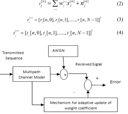
Figure 2. Adaptive Channel Estimator

2.1. Adaptive Channel Estimator

Fig.2 shows, the discrete time model of adaptive linear[2] channel estimation using LMS –like algorithms. The baseband equivalent channel impulse response is modeled as a transversal filter with M weights given in the vector

W(n) =[w0(n),w1(n)………wN-1]T (5)

Where the subscript n indicate the time index

We assume that the intersymbol interference is due solely to the propagation medium, which is modeled as an AWGN channel with discrete multipath intensity profile and delays spaced by the symbol duration. So the channel tap weights wi

(n)=0,1...,.M-1 are modelled as mutually uncorrelated complex Gaussian process with zero mean and variance and identical Doppler spectrum shape given in multipath intensity profile is the input vector composed of statistically independent and equiprobable complex modulation symbol with zero mean and variance σ2

Let d (n) be the desired response of the adaptive filter d(n) = xT_{(n)w(n) +n(n) (6)}

Where, x(n)=[x(n),x(n-1),...x(n-M+1]T

is the input vector composed of statistically independent and equiprobable complex modulation symbol with zero mean and variance σ2_.

The adaptive filter output is

y(n) = w(n) xT_{(n) (7)}

n(n) is the system noise that is independent of x(n) We express the estimation error as

e(n) = d(n) – y(n) (8) There are various algorithms are available for minimizing the weight w (n).The updating of µ(n) is required to use the autocorrelation of the error rather than the square of the error value.

2.1.1. LMS

In the LMS, the updatation is in such a way that the instantiation cost function

Jn = (e)2 ₍₉₎

The weight is updated by the steepest decent rule.

W(n+1) = w(n) -µ∂Jn/∂w(n) (10) The final weight will be

W(n+1) = w(n) -µe(n)x(n) (11) 2.1.2. RLS

The RLS channel estimation algorithm requires all the past samples of the input and the desired output is available at each iteration. The updating equation is

k = λ-1p.u/(1 + λ-1p x(n)' p x(n)) (12) w = w + k *conj(e(n)) (13) p = λ-1p - λ-1 p k x(n) (14) 2.1.3. VLLLMS

In VSLLMS[18]adaptive channel estimator the cost function Jn is the square of the estimated error.

Jn = (e)2 _{+ γ(n) + x(n) W(n) W}T_{(n) (15)}

Where γ(n) is the variable leakage factor which is defined as γ (n+1)= γ (n) - 2µ(n) ρ e(n) xT_{(n)w(n-1) (16)}

Constant ρ and whose value is greater than 1 The equation of the adaptive step size is

µ(n+1) = λµ(n) + γ(n)p2_{(n) (17)}

the autocorrelation of e(n) is

p(n) = βp(n-1) + (1-β)e(n)e(n-1) (18) where, 0<β<1

and finally weight is updated as

[image:3.595.62.308.255.474.2]

(4)

2.1.4. Derivation of the proposed modified LLMS algorithm The error signal at time n is given by

e(n) = d(n)- y(n) (20) Where d(n) is the desired signal

The output of the linear filter is given by

y(n) = wT_{(n)x(n) (21)}

Where x(n) is the input to the filter which is

x(n) =[x(n) x(n-1) x(n-2)……. x(n-L+2) x(n-L-1)]T

and w (n) is the filter gain

w(n) = [w(0) w(1) w(2)….. ……..w(n-L+2) w(L-1)]T

In adaptive filtering, the Wiener solution is found through an iterative procedure,

W(n+1) = w(n) + ∆w(n) (22) where ∆w(n) is an incrementing vector.

The instaneous cosy function defined as

Jn = e2_{(n) (23)}

w(n+1) = w(n)- µ∇ (e2_{(n)) (24)}

∇ is the gradient operator

∇ = [∂/∂w0 ∂/∂w1 ∂/∂w2 ... ∂/∂wN-1]T

∂e2_{(n)/∂wi = 2e(n) ∂ e(n)/∂wi}

= -2e(n) ∂ y(n)/∂wi = -2e(n)x(n) So Equ. (21) becomes

w(n+1) = w(n) +2e(n)x(n) (25) The cost function of the modified leaky LMS algorithm is defined by the following equation

Jn = e2_{(n) + γw}T_{(n)w(n) (26)}

Where 0 ≤ γ < 1 so as to avoid parameter drifting γwT_{(n) w(n) is a regularization component}

Selecting a constant γ may lead to over/under parameterization of this regularization component. One way to avoid this use variable γ.

Jn = e2_{(n) + γ(n)w}T_{(n)w(n) (27)}

Then the equation of weight updatation becomes

W(n+1) = e2_{(n) - µ∂Jn/∂w(n) (28)}

Where µ > 0 is a step size parameter to be chosen by the designer. Choosing a constant µ puts some weights on the correlation term throughout the estimation process that may suffer the convergence of the algorithm.

This feature may be incorporated using a variable step size updatation scheme for µ that yield a faster convergence.

W(n+1) = e2_{(n) - µ(n)∂Jn/∂w(n) (29)}

Where µ(n) is a variable step size parameter and may be updated as

µ(n+1) = γµ(n) + γ(n)e2_{(n) (30)}

In leaky LMS we are considering non stationary noise field, low SNR.Updating of µ(n) is required to use the autocorrelation of the error rather than the square of the error value to take care of the effect of the external disturbances in the step size update.

So equ.(11) modified as

µ(n+1) = λµ(n) + γ(n)P2_{(n) (31)}

where P(n) is the autocorrelation of e(n) and can be computed for an ergodic process by using a time average of it.

P(n+1) = βP(n) + (1- βe(n)e(n-1) (32) Where 0 < β < 1 is a forgotten parameter to be chosen by the designer. Choosing a constant β puts some weights on the convergence of the algorithm. and gives larger BER.To overcome this we use variable β(n) ,

β(n+1) = β(n) – logβ(n)/M (33) So equ.(13) modified as

P(n+1) = β(n)P(n) + (1- β(n)e(n)e(n-1) (34) Now we are ready to obtain the final update equation for w(n) and Now update the λ(n) and γ(n).

γ(n+1) = γ(n) – 4µ(n)ρ e(n) xT_{(n)w(n-1) (35)}

where ρ>1And finally weight is updated as

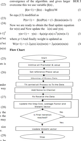
[image:4.595.279.546.270.736.2]

W(n+1) = (1-2µ(n) λ(n))w(n) + 2µ(n)e(n)x(n) (36) Flow Chart

(5)

64 Modified LLMS Algorithm for Channel Estimation in Noisy Environment

This flow chart fig 3 contents the total process step by step done in Modified Least Mean Square (MLMS) Algorithm for Channel Estimation in MIMO-OFDM System.

3. Computational Complexity

The evaluation of the inner products x(n)w(n) requires N complex multiplication and N complex additions for each iteration[4]. The multiplying the scalar by a vector requires N complex multiplications. We can compute the complexity of the LMS, VLLMS and Modified MLLMS algorithms. The following table summarizes the complexity cost in each iteration.

Table 1. Computational Complexity

Algorithms Multiplication Addition Division

LMS 2N+1 2N -

RLS N2_+5N+1 _N2_+3N ₁

VLLMS 4N 6N+3

MLLMS 5N 5N+3

4. Simulation Result

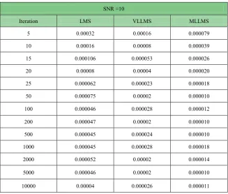
[image:5.595.141.469.365.643.2]

In this section we consider 2x2 MIMO-OFDM system. Simulate MLLMS algorithm for different SNR and iterations. Also compare the result with the standard LMS and RLS algorithm. For implementing the proposed MLMS algorithm, first requires setting the parameter µ, α and w and the initial values for µ, α, ρ and w. In the present work, we chosen µ, α, ρ, w=0 .BPSK signal with Gaussian noise is used to study the performance of the algorithms in presence of noise. Seven different cases of noises with signal-to-noise ratio (SNR) of 1 to 20 dB and iterations of 5 to 10000 are considered for the study shown in table 2 and 3. The corresponding results are shown in fig.4, fig.5 and fig.6.It can be observed that the BER reduces as the SNR increases from 1 to 20 dB .In MLLMS the forgetting factor β is adaptive in nature and whose value is adapt as per equation 33.by using the logarithmic we can overcome the problem of parameter drifting in the LMS algorithm.

Table 2. BER Comparison of algorithms for SNR=10

SNR =10

Iteration LMS VLLMS MLLMS

5 0.00032 0.00016 0.000079

10 0.00016 0.00008 0.000039

15 0.000106 0.000053 0.000026

20 0.00008 0.00004 0.000020

25 0.000062 0.000023 0.000018

50 0.000075 0.00002 0.000010

100 0.000046 0.000028 0.000012

200 0.000047 0.00002 0.000010

500 0.000045 0.000024 0.000010

1000 0.000045 0.000028 0.000018

2000 0.000052 0.00002 0.000014

5000 0.000046 0.00002 0.000010

(6)

[image:6.595.176.433.83.474.2]

Figure 4. BER Comparison of MLLMS with RLS for SNR=10

Figure 5. BER Comparison of LMS,VLLMS and MLLMS for SNR=10

[image:6.595.183.430.522.729.2]

(7)

[image:7.595.158.452.86.346.2]

Table 3. BER Comparison of algorithm for SNR=20

SNR =20

Iteration LMS VLLMS MLLMS

5 0.000200 0.000100 0.000049

10 0.000100 0.000050 0.000024

15 0.000067 0.000033 0.000016

20 0.000050 0.000025 0.000012

25 0.000039 0.000015 0.000011

50 0.000047 0.000013 0.000007

100 0.000030 0.000018 0.000008

200 0.000030 0.000013 0.000007

500 0.000028 0.000015 0.000007

1000 0.000028 0.000017 0.000011

2000 0.000032 0.000013 0.000009

5000 0.000029 0.000013 0.000006

10000 0.000026 0.000016 0.000007

5. Conclusion

A MLLMS algorithm has been used to estimate the channel in pilot aided MIMO-OFDM system. The BER performance of channel estimation was improved because the received data were subtracted from the desired signals. It has been shown using several simulations and experimental studies that this algorithm is superior to LMS,VLLMS and RLS for channel estimation. Although the proposed algorithm is slightly computationally complex compare to LMS. It has been observed that it is faster in convergence, more accurate and consistent with respect to several irregularities that are encountered in channel estimation schemes. Based on these observations use of MLMS is suggested for channel estimation in high data rate wireless communication.

6. Future Work

We will extend the work to compare with other algorithm by using other modulation techniques with different fading channels such as Rayleigh, recian. And furthermore reduces Symbol Error Rate or Bit Error Rate.

REFERENCES

[1] Kala Praveen Bagadi And Prof. Susmita Das,

“MIMO-OFDM Channel Estimation Using Pilot Carries”, International Journal of Computer

[2] Pei-Sheng Pan And Bao-Yu Zheng, “Adaptive Channel

Estimation Technique In MIMO OFDM Systems”, Journal Of Electronic Science And Technology Of China, Vol. 6, No. 3, September 2008.

[3] Sung won Jo, Jihoon Choi and Yong H. Lee,” Modified Leaky LMS Algorithm for Channel Estimation In DS-CDMA Systems”, IEEE Communications Letters, Vol. 6, No. 5, May 2002.

[4] Md. Kamal Hosain and Md.Masud Rana,”Adaptive Channel Estimation Techniques for MIMO OFDM Systems”, (IJACSA) International Journal of Advanced Computer Science and Applications, Vol. 1, No.6, December 2010 [5] Max Kamenetsky and Bernard Widrow, “A Variable Leaky

square algorithm-based power system frequency estimation”,IET Sci, Meas, Technol.,2012,

[7] Ye (Geoffrey) Li,”Simplified Channel Estimation For OFDM Systems With Multiple Transmit Antennas”, IEEE Transactions On Wireless Communications, Vol. 1, No. 1, January 2002

[8] Yushi Shen and Ed Martine, “Channel Estimation in OFDM Systems”, Freescale Semiconductor, Inc., 2006.

[9] E. Karami,“Tracking performance of least squares MIMO channel estimation algorithm”, IEEE Trans. On Wireless Comm. vol. 55, no.11,pp. 2201-2209

[10] Sinem Coleri, Mustafa Ergen, Anuj Puri, And Ahmad Bahai, “Channel Estimation Techniques Based On Pilot Arrangement In OFDM Systems”, IEEE Transactions On Broadcasting, Vol. 48, No. 3, September 2002.

(8)

2001

[12] S. Haykin, “Adaptive Filter Theory”, 4th Ed. Upper Saddle River, Nj: Prentice Hall, 2002.

[13] Thomos Hesketh,Rodrigo C,de Lamare “Adaptive MMSE channel estimation algorithm for MIMO systems” European Wireless 2012,April 18-20 2012 Poznan Poland.

[14] Mehmet Kemal Ozdemir logus,Huseyin “Channel Estimation for wireless OFDM systems”IEEE communication surveys 2007, volume 9,No2

[15] Junghsi Lee,Jia-Wei Chen and Hsu-Chang Huang

“Performance comparison of variable step size NLMS

algorithms”World congress on Engineering and Computer Science 2009 Vol 1 San Francisco,USA.

[16] K.Mayyas and Tyseer Aboulnasr “Leaky LMS algorithm : Analysis for Gaussion data” IEEE transaction on signal Processing Vol.45,No 4 April 1997

[17] William A. Sethares, Dale A. Lawrence C. Richard Johnson, Robert R. Bitmead.” Parameter Drift in LMS Adaptive Filter” IEEE transactions on Acoustic, speech and signal processing,Vol ASSP 34 No 4 August 1986