Probabilistic Classification from a
K-Nearest-Neighbour Classifier
Charles D Mallah
∗,
James Orwell
Kingston University, Kingston upon Thames, London, United Kingdom
∗Corresponding Author: [email protected]
Copyright c2013 Horizon Research Publishing All rights reserved.
Abstract
K-nearest-neighbours is a simple classifier, and with increasing size of training set, the accuracy of its class predictions can be made asymptotic to the upper bound. Probabilistic classifications can also be generated: the accuracy of a simple proportional scheme will also be asymptotic to the upper bound, in the case of large training sets. Outside this limit, this and other existing schemes make ineffective use of the available information: this paper proposes a more accurate method, that improves the state-of-the-art performance, evaluated on several public data sets. Criteria such as the degree of unanimity among the neighbours, the observed rank of the correct class, and the intra-class confusion matrix can be used to tabulate the observed classification accuracy within the (cross-validated) training set. These tables can then be used to make probabilistic class predictions for the previously unseen test set, used to evaluate the novel and previous methods in two ways: i) mean a posteriori probability and ii) accuracy of the discrete prediction obtained from integrating the probabilistic estimates from independent sources. The proposed method performs particularly well in the limit of small training set sizes.Keywords
Pattern Recognition, Plant Leaves Clas-sification, k-Nearest Neighbours, Density Estimators, Combining Features1
Introduction
The ‘K-nearest neighbour’ (K-NN) classifier is a
fun-damental tool for pattern analysis, providing a straight-forward means of estimating to which class a previously unseen sample vector belongs, given a finite training set. It naturally generalises to problems with multiple classes; for a ‘test’ set of unseen vectors, the resulting precision and recall statistics provide an insight into the separability of the problem. Moreover, its performance can be improved using metric learning approaches [14], and accelerated with enhanced implementations [9]. In this paper, methods are examined for using the training set to estimate the class membershipprobabilities for a
test vector. A novel approach is proposed, which has the dual advantages of a fast, non-iterative implementation, and also providing significantly more accurate estimates than the state-of-the-art, over a range of test sets. One challenging set comprises images of leaf specimens from one-hundred species; a sample of which is shown in Fig-ure 1.
The standardK-NNclassifier requires a single
param-eter,K, to select theKnearest elements in the training set: the single most popular class label in this subset is output as thediscreteestimate. There are some possible variations of a nearest neighbours system in the type of distance measure used and in the tie-break mechanism. With increasing size of training set, the accuracy of the
K-NNdiscrete estimate tends towards the lowest
possi-ble – the Bayes error rate – if Kcan be increased along with the training set size, or twice this rate otherwise [3]. However, the focus of the current work is with small training set sizes: the objective is to use the limited data available as efficiently as possible.
(a) (b) (c) (d) (e) (f)
[image:1.595.312.554.513.620.2](g) (h) (i) (j) (k) (l)
Figure 1. A small variety of plant species that are part of the challenging one-hundred species leaves data set: (a) Acer Campestre. (b) Acer Circinatum. (c) Acer Mono. (d) Acer Pal-matum. (e) Alnus Rubra. (f) Alnus Sieboldiana. (g) Betula Aus-trosinensis. (h) Eucalyptus Urnigera. (i) Ilex Aquifolium. (j) Ilex Cornuta. (k) Liquidambar Styraciflua. (l) Liriodendron Tulip-ifera.
A probabilistic estimate of class label is not part of the standard output of the K-NN. However, the
use-ful development [1] is to allocate a weight to each mem-ber of the training set, and then optimise these weights to maximise the likelihood of this training data. These methods are further described in Section 2. There are also other approaches to density estimation: parametric methods such as Expectation-Maximization of Gaussian Mixture models [12], and non-parametric Kernel-based methods [2, 8] that generalise the histogram-based ac-cumulation of samples. These are not included in this investigation because they are not suitable at the op-erating range of interest, i.e. problems with scores of classes in hundreds of dimensions, with only a handful of data points per class.
For discrete estimates, the evaluation of a classifier’s performance is straightforward: precision and recall can be combined into a single ‘mean accuracy’ characteris-tic. The most appropriate evaluation of probabilistic es-timates is to report the mean log likelihood of the unseen test data: this is maximised when the Bayes estimate of the p.d.f. is used, and in general its expectation will differ by the Kullback-Leibler distance from the p.d.f. Most importantly, probabilistic estimates from different sources can be combined together much more effectively than discrete estimates. If the sources are conditionally independent then this is a straightforward multiplica-tion: this enables evidence to be combined with prior probabilities, or the separate available channels of evi-dence to be combined together.
A framework is proposed to tabulate statistical prop-erties of the neighbours from within the training set, and how these characterize the classification performance. These properties can be combined in a robust and straightforward (non-iterative) approach. Within the framework, theK-NNclassifier is used to provide
statis-tics about its expected performance within the training set, which are then used to provide estimates for the unseen test set process. The proposed approach is com-pared against the standard [6] and the recent extension [1].
The paper is organized as following: Section 2 de-scribes the notation and evaluation of the state-of-the-art of probabilistic estimators in aK-NNsystem.
There-after, in Section 3, the novel work is described to define a series of estimators based on tabulation of statistics. Section 4 describes the public data sets used to evaluate the estimators, in addition to the experimental results per data set. The paper is concluded in Section 5, which includes comments on further work.
2
Probabilistic Estimators
Let the training set of n vectors, Y, be denoted by
{y1, . . . , yn}and the test setX is formed bymvectors
{x1, . . . ,xm}. Both sets are labelled using {y1, . . . , yn} and{x1, . . . , xm}, respectively, where each label one of theC discrete classes (or categories) 1, . . . , C. For con-venience, an identity operatorI(·) is defined to obtain a vector’s label, i.e. label, i.e. I(xi)≡xi, and in particu-larp(I( xi)=j)≡p(xi=j).
Formally, the objective is to calculate the estimator ˆ
p(·) to be as close as possible to the Bayes estimate
p∗(xi=j), i.e. the probability that a given test vector
has labelj, where 1≤j≤C.
This can be factored into a likelihood term and a prior probability that sampleiis of labelj:
ˆ
p xi=j
| {z }
posterior
= ˆL xi=j
xi,Y
| {z }
likelihood
π(xi=j)
| {z }
prior
(1)
Typically, for experimental purposes, the prior terms are often all set to be equal; though naturally, in prac-tical applications they may have specific values deter-mined by the circumstances. The posterior estimator is an estimate of the unknown, optimal, Bayes estimate
p∗(·).
Note that, firstly by assuming an exhaustive and ex-clusive labelling, both ˆp(·) and p∗(·) will sum to unity over theCclasses. Secondly, the Bayes estimatep∗(·) is optimal in the sense that it minimises the posterior ex-pected loss over the unseen test set{xi}, across all pos-sible estimates ˆp. Thirdly, the appropriate evaluation measure for any given estimate, is the Kullback-Leibler distance D(p∗(·),pˆ(·)). However, since in general p∗(·) is unknown, one way to report the accuracy of a partic-ular estimator ˆpAis by evaluating its mean log posterior
LPA, using a sufficiently large unseen test setX:
LPA= m
X
i=1
log ˆpA I(xi)=xi (2)
This expression quantifies the extent to which this es-timator ‘picked the right horse to win the race’, i.e. the value of ˆp(x)i for the correct labelxi . This quantity is maximised for the Bayes estimatorp∗, and it can be used to compare the relative accuracies of any two methods
AandB, with estimators ˆpAand ˆpB. One aspect of this metric is that it diverges to−∞if∃i: ˆp I(xi) =xi) = 0. As a consequence, the estimator fails to assign a finite probability to an event that did indeed transpire. To address this problem, an estimator should assign finite probabilities to all possible label assignments.
Alternatively, the accuracy of the estimates can be evaluated by combining evidence from S multiple sources, i.e. the set of training sets{Y1, . . . ,YS}, where the vectors in each set have their own associated fea-ture space. If these sources are independent, then the combined estimate ˆq(·), using these estimators for these features is:
ˆ
q(xi=j|Y1. . .YS) = S
Y
s=1 ˆ
p(xsi=j|Ys) C X c=1 S Y s=1 ˆ
p(xsi=c|Ys) (3)
2.1
The Proportional (Prop) EstimatorThe standard approach [6] is to define a proportional estimator, ˆpProp(·), as follows. For any given input vec-tor xi, the subset ofK nearest training set neighbours is ordered according to their ascending distance to the considered sample {yi
1, . . . ,yki, . . . ,y i
estimate ˆp0 of the probability that xi belongs to
cate-goryj, is constructed proportionally to Ki(j)/K. It is shown that in the case of large training set size, Equa-tion 4 converges to the definiEqua-tion of probability density. Figure 2 illustrates the Prop estimator and the Bayes
Risk.
Furthermore, the estimator is not very efficient at making use of the available information. For instance, it assigns zero probability to those outcomes forxilacking any ‘precedent’ in the training set, i.e. for which, among the K members of the training set nearest to xi, none have a matching category, so Ki(j) = 0. To overcome this problem, a constant proportion of the probability mass, ∆, is allocated to account for this chance of ‘model failure’, shared out equally among theC classes:
ˆ
pProp(xi=j) =
(1−∆)Ki(j)
K +
∆
C (4)
A similar approach is integrated into all types of esti-mator investigated here. While it is possible to optimise the value assigned to ∆, it would take very large, sta-tionary data sets to get any meaningful results, since it is effectively insurance against rare outcomes.
2.2
The Weighted Proportional (wProp) Esti-matorAtiya [1] generalises this idea by proposing the assign-ment of an unconstrained weightwk to each member of the training set yk, using a sigmoid function to trans-form this intogk, which always lies in the unit interval. As a result, an estimate is given by the following equa-tion:
ˆ
pwProp(xi=j) =
(1−∆)Ki(j)
K
K
X
k=1
gkδ(yk=j) + ∆
C
(5) where theδ(·) picks out only those neighbours of cate-goryj, and ∆ is once again the term to guard against model failure.
The key advantage is that, within the training set, the set of unconstrained weights{wk}can be optimised to maximise the likelihood of the training set given this estimator: the cost function can be shown to be con-vex with the appropriate stationary point. Thanks to this, the efficient search approach by gradient-ascent is applied to find the optimal set of weights.
3
Tabulation of Prior Statistics
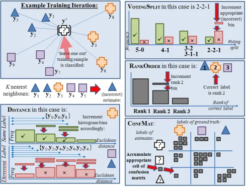
To construct an accurate estimate of the posterior probability, it is proposed to investigate various defini-tions of table that can be used to accumulate statistics from the training set. These tables can be combined and used to record the varying degrees of certainty that have been encountered across the sections of the input space. Hence, for an unseen test vector, its relation to its near-est neighbours in the training set can be used to identify similar sections of the input space, and simply look up the probability that has been measured from the cross-validated statistics. Figure 3 illustrates the proposed framework.
To tabulate these statistics from the training set, a ‘leave-one-out’ cross validation is applied. This means that features are extracted and accumulated, leaving out a single member of the training set. These features are used to predict the label of the left-out sample: the sult is stored as a prior statistic. This process is re-peated n times, to assemble a table of the prediction performance, conditioned upon the different values that the extracted features can assume. In general, discrete features were chosen, in preference to continuous ones: this allows a tabulation as opposed to a regression. An important design decision is the number of possible fea-ture values, i.e. the number of elements in the condi-tional tables: a fine-grained model can provide more de-tail, while a course-grained model allows more statistics to accumulate per element which provides more reliable predictions.
We propose to use four different features of the train-ing set to generate the prior statistics: VoteSplittable, Rank table, Dist feature, and ConfMat (confusion
ma-trix). These are presented in the subsequent sections (3.1 to 3.4). These tables are then combined together in various ways to generate several estimators that can be evaluated on test sets alongside the PropandwProp
methods. The methods for combining the tables are de-scribed in section 3.5.
3.1
The VoteSplitTableIt is hypothesised that the degree of agreement be-tween the K nearest neighbours to xi provides a use-ful indication about the certainty of the classification result. Intuitively, a unanimous verdict from the K
nearest neighbours is a more certain result, than some equivocation between two or more labels. This degree of agreement can be simply modelled by a histogram with
K bins: each element k of the histogram is used for those cases in the training set in whichk of the nearest neighbours have the same label as the predicted result. The histogram is used to accumulate and then calcu-late the proportion of these cases in which the predicted result is correct. This is achieved using the ‘leave-one-out’ methodology to fabricate mtest cases from within the training set, in each case omitting it from the list of neighbours used to determine its result.
An example of the accumulation of the VoteSplit
ta-ble, in addition to the remaining three features, is shown in figure 4.
3.2
The RankOrder of Correct Labelshis-Figure 2. Supposing estimates of posterior probability density functions for two classes are required: thePropestimator uses the proportion of theKneighbours found to have that class label in each case. As the overall density (number) of available neighbours increases, this estimate will converge on the true p.d.f. However, it makes inefficient use of the available information. Also shown is the ‘Bayes Risk’; which is the expectation of minimum risk due to some inevitable errors.
togram is normalised to provide an indication of relative frequency.
3.3
Conditional Dependence on DistThe accumulation of statistics to measure the recorded (Euclidean) distance between samples that are either the same label or different labels, is well estab-lished in the literature [15]. In this context, the set
{|y0 −yk|} denote the distances between the
cross-validation probey0 and itsK nearest neighbours{yk}.
The distances are quantised into the histogram bins; for those distances for which the neighbour and the probe have the same label, i.e. y0=yk, histogramH1is incre-mented. Otherwise, histogramH2 is incremented.
To obtain a probability that is conditioned upon a given quantised distance (and histogram bin) b, the histograms are normalised to their respective priors and then the conditional probability is H1(b)/(H1(b) +
H2(b)).
3.4
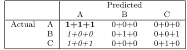
The ConfMat Confusion MatrixThe confusion matrix [13], ConfMat, is a standard
methodology for cross-validation; whereby a matrix of relative performance of a classifier per class is visualised in a specific table layout. Each column of the matrix represents the instances in a predicted class, while each row represents the instances in an actual class; for each associated correct or incorrect prediction, a 1 value is tallied to the respective row and column of the table. This represents the frequency over the training set that
categoryj1is classified as categoryj2. An example con-fusion matrix is shown in table 1. The ConfMat table
[image:4.595.58.533.52.350.2]uses the classifier precision from each class in the confu-sion matrix as the direct probabilistic estimate for any future prediction of that specific class.
Table 1. Example confusion matrix with three class labels: A, B, and C, and three samples of each class. The relative tallies can be evaluated in various ways to provide estimates of the classification accuracy. In the case of class A there are three true positives, where A was correctly predicted; three false positives, where one B sample and two C samples were confused to be as class A; no false negatives; and lastly three true negatives. The respective classification accuracy (precision) for class A would therefore be equal to: 3+33 = 0.50 (where the true positives for class A are shown in bold, and the false positives shown in italics).
Predicted
A B C
Actual A 1+1+1 0+0+0 0+0+0 B 1+0+0 0+1+0 0+0+1 C 1+0+1 0+0+0 0+1+0
3.5
Combination of TablesCombinations of the various feature tables can be im-plemented to create additional novel estimators. In the simplest combination, an additional column is added to the table, which provides more discrimination between various values in the table. Some of the combinations are documented as the following:
1. The Dist&VoteSplit estimator: This combined
[image:4.595.322.510.612.662.2]frame-Figure 3. The proposed novel density estimator framework using tabulated statistics calculated from an internal data-set. A posterior estimate for the unseen query sample can then be calculated using the prior estimates. The evaluation method is also illustrated, whereby each probabilistic estimate per feature can be combined to produce various class predictions. The selected classifier features used to build the estimator, in addition to the test sample feature combinations, can thus be evaluated like-for-like, (allowing a selection of the preferred classification solution).
work. For additional granularity, the table contains two columns: the first remains as distance with the second adding the range of categories from the
VoteSplittable.
2. The Rank&VoteSplit matrix estimator: Similar to
the above method, however instead of using the dis-tance feature uses theRankfeature as the first
col-umn of the table, and the VoteSplit table as the
second.
3. The ConfMat&Rankestimator: Whereby
probabil-ity mass is accumulated into the confusion matrix instead of the discrete 1 assigned if the prediction matches the ground truth. In this case, the proba-bility mass from theRanklookup table is calculated
and accumulated in the relevant row and column of the confusion matrix (see section 3.4). This new confusion matrix requires normalisations so that the total probability mass across each row of the matrix sums to one; this also means that there are no zero-value elements in this table (to avoid model failure), therefore all elements have a constant value added to them (such as +1). TheConfMat&Rankmatrix is
then used in the same way as the standardConfMat
table. An example is shown in table 2.
4. The ConfMat&Rank&VoteSplit estimator:
Simi-lar to the above method, however instead uses the additional information from the combined
Rank&VoteSplit table to estimate the probability
mass which, again, in turn is accumulated into the
ConfMatmatrix instead of discrete 1 values.
Table 2. Example confusion matrix, aggregating probability mass instead of discrete values. In this example, the results are roughly equivalent to table 2 The respective classification accu-racy (precision) for each class is readily available after adding a constant value to each element (such as 1), then normalise each row by the total of that row (so the sum becomes equal to 1).
Predicted
A B C
Actual A 0.9 + 0.85 + .78 0 + 0 + 0 0 + 0 + 0 B 0.4 + 0 + 0 0 + 0.75 + 0 0 + 0 + 0.43 C 0.85 + 0 + 0.7 0 + 0 + 0 0 + 0.8 + 0
4
Experimental Evaluation
The following estimators are tested in this paper:
[image:5.595.57.553.49.411.2]Figure 4. An example iteration of the accumulation of the tabulated statistics: VoteSplit,Rank,Dist, and ConfMatfeatures. These features would eventually be tabulated over all of the training iterations, using each training sample as a new leave-one-out test sample.
statistics (Section 3). The eight estimators are evalu-ated using unseen test sets. Results are accumulevalu-ated using ten-fold evaluation (for Iris and Wheat data sets) and sixteen-fold evaluation of the leaves data set. In each of these iterations, the estimator is rebuilt com-pletely, thus ensuring that a sample used as a test vec-tor in one iteration, can be used as a training vecvec-tor in another iteration, without compromising the integrity of the experiments. In all cases there are an equal number of samples used from each class, effectively setting the priors to be equal. The performance results reported consist of the mean log posterior (LP), i.e. expected log likelihood, of the density estimates and the mean classifi-cation accuracy (Acc) of the estimators. For the results
concerning the Leave data set, we additionally report the mean precision and mean recall accuracies (due to the number of classes and complexity of the data set).
For each estimator, the number of separate features to be included in the classification can be varied. Each feature has its own separateK-NNsystem that is trained
on the respective training data. There are two, three and four separate K-NN systems created, for the Iris,
Leaves and Wheat data sets; the Leaves features are multivariate (64-dimensions each); the Iris and Wheat features are univariate. In the current investigation, the
K-NN system is configured with a Euclidean distance
measure and the first-nearest neighbour is used as the tie-break mechanism. Additionally, the ‘model failure’ value of ∆ = 0.01 is used for all experiments, i.e. 1% of the probability mass is reassigned to all classes thus removing zero valued elements (Section 2.1).
In each case, the evaluation reports two measures of performance: the log posterior of the probabilistic es-timate, and the accuracy of the final discrete estimate. The main objective of the experiments is to understand which of the available estimators provides the most ac-curate classification results. Subsequently, the perfor-mance as a function of training size is investigated, using the high-dimensional (Leaves) data set.
4.1
Test Data setsTwo public benchmark data sets are employed to vali-date the performance of considered methods: Iris Flower and Wheat Seed Kernel (Section 4.1.1). The experimen-tal design restricts the processing of these data sets to a single variable perK-NNclassifier, to examine the
4.1.1 Iris Flowers & Wheat Seed Kernels
A well-known data set in the pattern recognition liter-ature is Fisher’s iris data [5, 4]. It consists of 50 samples from 3 varieties of Iris plant. The features of the iris data consist of four scalar values; these refer to the Length and Width of the Petal (PL and PW), and the Length
and Width of the Sepal (SL and SW). Guvenir et al,
[7], use the iris data set (amongst others) to validate the performance of their own weighted K-NN classifier. In
the case ofK= 3, using a ten-fold cross-validation eval-uation, the mean classification accuracy was reported to be 90.7% for the standard classifier definition. The authors report an accuracy of 94% using their weighted
K-NNmetric (with the sameK= 3 parameter). We
cre-ate four separcre-ate feature vectors per iris sample, which relate to each of the petal and sepal dimensions (rather than use all values in one feature vector).
Another publicly available data set consists of seven attributes of wheat seed kernels [10]. The data set con-sists of 70 samples from 3 different varieties of wheat. The attributes refer to the Area (AR), Perimeter (PE),
Compactness (CO), Length of Kernel (LK), Width of
Kernel (WK), Asymmetry Coefficient (AS) and Length of
Kernel Groove (LKG). The authors report a mean
clas-sification accuracy of 92% using a clustering algorithm technique. Similarly to the Iris data set, we create sepa-rate feature vectors using each of these attributes within the test framework.
4.1.2 Plant Leaves
The ‘leaves’ data set comprises one-hundred species of leaves [11]. For each species, there are sixteen distinct specimens, photographed as a colour image on a white background. Figure 1 contains a sample set of silhouette images. From these samples, three distinct features were extracted: a Centroid Contour Distance Curve shape signature (Sha), an interior texture feature histogram
(Tex), and a fine-scale margin feature histogram (Mar).
Each feature is represented by a 64 element vector. The data set inherently consists of having a wide set of classes with a low number of samples. Additionally, many sub species resemble the appearance of other ma-jor species, as well as many sub species with a mama-jor species can resemble a radically different appearance. As such, this data set provides the main classification challenge from the three data sets described in this pa-per.
4.2
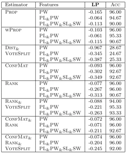
Iris Flower & Wheat Seed ResultsThe experimental results using the Iris Flower data set is shown in Table 3. All described density estimation methods were tested in this case withK= 3. Note, no significant differences were observed when experiments were conducted with K = 5 and K = 7. The results using the Wheat Seeds data set is shown in Table 4. Some minor differences were noted when experimenting withK= 5 andK= 7, however we include results using
[image:7.595.329.534.80.327.2]K= 3. For both cases, results of three different feature combinations are shown for comparative purposes.
Table 3. Experimental results using the Iris Flower data set.
Estimator Features LP Acc
Prop PW -0.165 96.00
PL&PW -0.064 94.67
PL&PW&SL&SW -0.113 90.00
wProp PW -0.103 96.00
PL&PW -0.061 95.33
PL&PW&SL&SW -0.115 90.67
Dist& PW -0.967 28.67
VoteSplit PL&PW -0.345 24.67
PL&PW&SL&SW -0.387 25.33
ConfMat PW -0.093 96.00
PL&PW -0.302 92.67
PL&PW&SL&SW -0.349 92.67
Rank PW -0.077 96.00
PL&PW -0.267 96.00 PL&PW&SL&SW -0.313 90.67
Rank& PW -0.088 94.00 VoteSplit PL&PW -0.221 95.33
PL&PW&SL&SW -0.263 93.33
ConfMat& PW -0.072 96.00
Rank PL&PW -0.071 96.00
PL&PW&SL&SW -0.211 92.67
ConfMat& PW -0.074 96.00
Rank& PL&PW -0.204 96.00
[image:7.595.310.556.375.624.2]VoteSplit PL&PW&SL&SW -0.245 92.00
Table 4. Experimental results using the Wheat Seed data set.
Estimator Features LP Acc
Prop AR&AS&LKG -0.182 88.10
PE&WK&AS&LKG -0.133 88.57
AR&PE&CO&LK&AS&LKG -0.137 88.57
wProp AR&AS&LKG -0.171 87.62
PE&WK&AS&LKG -0.134 88.57
AR&PE&CO&LK&AS&LKG -0.169 87.62 Dist& AR&AS&LKG -0.177 78.57
VoteSplit PE&WK&AS&LKG -0.192 81.43 AR&PE&CO&LK&AS&LKG -0.162 86.19
ConfMat AR&AS&LKG -0.172 86.67 PE&WK&AS&LKG -0.163 88.57
AR&PE&CO&LK&AS&LKG -0.183 89.05
Rank AR&AS&LKG -0.163 90.48
PE&WK&AS&LKG -0.154 88.57
AR&PE&CO&LK&AS&LKG -0.184 88.10
Rank& AR&AS&LKG -0.159 90.48
VoteSplit PE&WK&AS&LKG -0.148 87.14
AR&PE&CO&LK&AS&LKG -0.181 87.14
ConfMat& AR&AS&LKG -0.152 92.38
Rank PE&WK&AS&LKG -0.143 90.00
AR&PE&CO&LK&AS&LKG -0.183 89.52 ConfMat& AR&AS&LKG -0.151 90.00
Rank& PE&WK&AS&LKG -0.143 87.14 VoteSplit AR&PE&CO&LK&AS&LKG -0.185 87.62
4.3
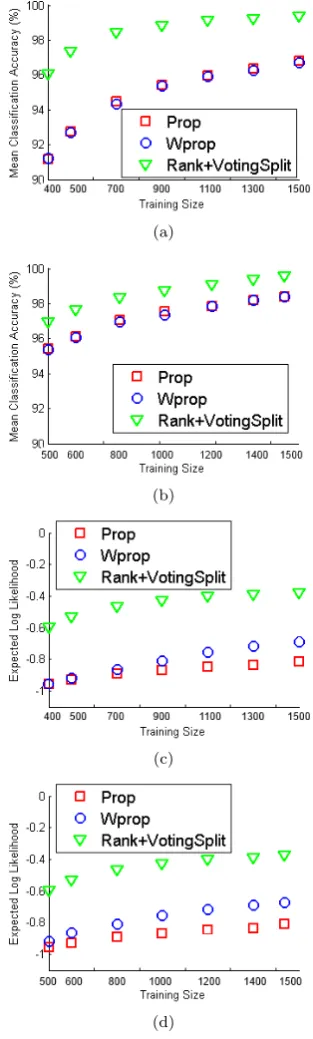
Plant Leaves ResultsThe experimental results using the plant leaves data set is shown in Table 5. All described density estimation methods were tested in this case withK= 3 andK= 5. The results shown consist of the combinedSha&Tex&Mar
classified features (unanimously, the best feature combi-nation across all estimators for the leaves data set). In addition to the mean classification accuracy, we report the mean precision and mean recall metrics in order to provide more detail on the performance of the estimators using this more complex data set.
metric. The respective plots are shown in Figure 5.
Table 5. Results of the sixteen-fold evaluation of the leaves data set using only theSha&Tex&Marfeatures combination.
Estimator K LP Acc Pre Rec
Prop 3 -0.814 96.81 96.98 96.81
5 -0.569 98.19 98.33 98.19
wProp 3 -0.554 96.69 96.87 96.69
5 -0.368 98.19 98.31 98.19
Dist& 3 -0.394 97.75 97.88 97.75
VoteSplit 5 -0.282 97.81 97.97 97.81
ConfMat 3 -0.327 92.25 92.96 92.25
5 -0.251 90.13 91.22 90.13
Rank 3 -0.263 99.25 99.31 99.25
5 -0.202 99.31 99.36 99.31
Rank& 3 -0.221 99.38 99.42 99.38
VoteSplit 5 -0.170 99.38 99.42 99.38
ConfMat& 3 -0.197 97.69 97.88 97.69
Rank 5 -0.155 97.19 97.31 97.19
ConfMat&Rank& 3 -0.189 94.63 94.75 94.56
VoteSplit 5 -0.158 91.81 92.29 91.81
4.4
Algorithm Computation SpeedThe experiments introduced in this paper were con-ducted on a workstation using the Microsoft Windows XP operating system with a 3.2 GHz processor and 3 GB of RAM; the algorithm was implemented in the MAT-LAB programming environment. We report the mean experiment time taken to classify one trial of the one-hundred species leaves data set, i.e. the average time to compute one-fold of 100 test samples using 1500 train-ing samples. Note that one trial comprises of buildtrain-ing a separateK-NNdensity estimator foreach feature vector
i.e. the classification timings noted here indicate timing of the entire experiment using all features. Our imple-mentation of thePropestimator had completed this task
in 21.8 seconds, whereas thewPropestimator was
com-pleted in 31.7 seconds. The Dist&VoteSplit estimator
performs slowest with 41 seconds processing time, and the remaining estimators all completed within 33 sec-onds.
4.5
DiscussionThePropandwPropestimators perform similarly with
respect to mean classification accuracy over the ten-fold cross-validation evaluation. Using the Iris Flower data set, a 96% mean accuracy with thePWfeature alone and
90% with all four of thePL&PW&SL&SWfeatures. With
regards to the expected log likelihood using thePW
fea-ture alone: -0.165 to -0.103 forPropandwProp,
respec-tively. For all estimators the single PWfeature worked
better than any combination of thePL,PW,SL, andSW
features. Comparatively, Guvenir et al [7] reported an accuracy of 94% using their proposed weighted K-NN
metric using all four values. All of the tested estimators performed less than this, however the Rank&VoteSplit
method was closest with 93.33% mean accuracy using the four features.
Similarly to the Iris Flower data set, results using Wheat Seeds show that many of the features combined together from the seven available did not give the op-timal solution. Generally, the framework worked
opti-(a)
(b)
(c)
(d)
Figure 5. Estimator performance as a function of training size using the leaves data set: UsingK= 3, (a) and (c) show the mean classification accuracy and expected log likelihood, respectively. Similarly, (b) and (d) show the results usingK= 5.
mally with the AR, AS, and LKG features. We observe
that of all estimators, the ConfMat&VoteSplitmethod
performs the strongest with a mean classification accu-racy of 92.38% and expected log likelihood of -0.152, us-ing the combination of AR&AS&LKGfeatures.
Compar-atively, Charytanowicz et al [10] reported a mean clas-sification accuracy of 92% using a proposed clustering algorithm on the same data set using all seven features. TheRank&VoteSplitestimator performed next best with
90.48% mean accuracy and mean log posterior of -1.159 (also using theAR&AS&LKGfeatures).
Leaves have further supported the performance of the
Rank&VoteSplitestimator. The mean classification
ac-curacy for the sixteen-fold evaluation was 99.38%, with an expected log likelihood of -0.17 (usingK= 5). Com-paratively, thePropandwPropmethods performed well
with a mean classification accuracy of 98.19%, respec-tively. The expected log likelihood for these methods were -0.569 and -0.368, respectively.
The K parameter selection from K = 3 to K = 5 had shown a 1.38% and 1.5% boost in classification ac-curacy for the Prop and wProp methods. However the Rank&VoteSplitmethod worked consistently across the
two tested K values. The remaining estimator meth-ods performed with varying success, most notably the
ConfMat based methods worked worse for the plant
leaves data set.
5
Conclusion and Further Work
This paper has introduced a novel framework for esti-mating the posterior probability density, using informa-tion available to a K-nearest neighbour classifier. Four different types of statistics were tabulated from within the training set, and various ways of combining these tables were investigated. Experiments on several data sets indicated that the best performing estimator is the joint table that conditions the estimate on theVoteSplit
and theRankof the hypothesis provided byK-NN.
For the one-hundred species leaf data set, integrat-ing all three Sha, Tex and Mar features, the novel Rank&VoteSplit method was the best performing
esti-mator. This was inferred from the standard discrete metric (99.38% mean classification accuracy). For the standard probabilistic metric (mean log likelihood of the test set), the values obtained from the combinations of
Rank,VoteSplitandConfMatwere in the range of -0.155
to -0.21, compared to the values obtained from the con-ventional estimators of -0.814 and -0.368. Thus these represent very sizeable improvements in the accuracy with which an unseen test set’s classification probabili-ties are estimated.
As a function of the training set size, the dis-crete classification performance is readily interpreted: at low values of available samples, and especially for low values of K (number of nearest neighbours), the
Rank&VoteSplit estimator provides significantly better
performance. Thus, the effectiveness of the framework is shown when combining the probabilistic estimates from individually processed features. For the leaves data set, the optimal configuration used all available features; however, this may not always be the case as shown with the iris flower and wheat seeds data sets. It has been shown to be effective in the particular task of classifi-cation with low training samples and a relatively large variety of categories.
There are several avenues of future work. For leaf recognition, it will be useful to validate the framework with noisy and missing data, e.g. missing parts of the sample leaf or focus errors. More generally, there are other areas of probabilistic estimation for which the pro-posed framework may be useful, e.g. correct estimation of face or vehicle registration plate details apparently permit a similar analysis. The evaluation of probability density will extend to check that kernel-based methods
and Parzen windows do not offer any advantage under these conditions. Finally, it will be useful to investigate the extent to which properties of the training set statis-tics can predict the out-of-sample performance on the test set, to enable the most appropriate combination of tabulated data to be automatically selected and used.
REFERENCES
[1] A. F. Atiya. Estimating the posterior probabilities using the k-nearest neighbor rule. Neural computation, 17(3): 731–740, 2005.
[2] A. W. Bowman. A comparative study of some kernel-based nonparametric density estimators.Journal of Sta-tistical Computation and Simulation, 21(3-4):313–327, 1985.
[3] T. M. Cover, J. A. Thomas, and J. Wiley. Elements of information theory, volume 6. Wiley Online Library, 1991.
[4] R. O. Duda and P. E. Hart. Pattern recognition and scene analysis. 1973.
[5] R. A. Fisher. The use of multiple measurements in tax-onomic problems.Annals of Human Genetics, 7(2):179– 188, 1936.
[6] K. Fukunaga and L. Hostetler. K-nearest-neighbor bayes-risk estimation. Information Theory, IEEE Transactions on, 21(3):285–293, 1975.
[7] H. A. Guvenir and A. Akkus. Weighted k nearest neigh-bor classification on feature projections 1. 1997.
[8] J. N. Hwang, S. R. Lay, and A. Lippman. Nonpara-metric multivariate density estimation: a comparative study.Signal Processing, IEEE Transactions on, 42(10): 2795–2810, 1994.
[9] W. J. Hwang and K. W. Wen. Fast knn classification algorithm based on partial distance search. Electronics Letters, 34(21):2062–2063, 1998.
[10] P. Kulczycki and M. Charytanowicz. A complete gra-dient clustering algorithm. Artificial Intelligence and Computational Intelligence, pages 497–504, 2011.
[11] Charles Mallah, James Cope, and James Orwell. Plant leaf classification using probabilistic integration of shape, texture and margin features. Signal Processing, Pattern Recognition and Applications, 2013.
[12] T. K. Moon. The expectation-maximization algorithm.
Signal Processing Magazine, IEEE, 13(6):47–60, 1996.
[13] Stephen V Stehman. Selecting and interpreting mea-sures of thematic classification accuracy. Remote sens-ing of Environment, 62(1):77–89, 1997.
[14] K. Q. Weinberger and L. K. Saul. Distance metric learning for large margin nearest neighbor classification.
The Journal of Machine Learning Research, 10:207–244, 2009.