Munich Personal RePEc Archive
Changes in Environmentally Sensitive
Productivity and Technological
Modernization in China’s Iron and Steel
Industry in the 1990s
Fujii, Hidemichi and Kaneko, Shinji and Managi, Shunsuke
2009
Changes in Environmentally Sensitive Productivity and Technological
Modernization in China’s
Iron and Steel Industry in the 1990s.
Abstract. Technological modernization is widely believed to contribute positively both to
economic development and to environmental and resource conservation, through productivity
improvements and strengthening of business competitiveness. However, this may not always
be true, particularly in the short term, as it requires substantial investments and may impose
financial burdens on firms undertaking such investments. This study empirically examines the
effects of technological modernization in China’s iron and steel industry in the 1990s on conventional economic productivity (CEP) and environmentally sensitive productivities
(ESPs). We employ a directional distance function that can handle multiple inputs and outputs
to compute relative production efficiencies. We apply these models to the data covering 27
iron and steel firms in China between 1990 and 1999—a period when the Chinese iron and steel industry modernized rapidly. We find that ESPs have continuously improved, even in the
1 Introduction
China’s economic growth has been extremely rapid, with an annual growth rate of approximately 10% over the last two decades (Asian Development Bank, 2007). The resulting
economic development has created environmental and resource problems that threaten China’s sustainability (De Groot et al., 2004)1. The annual economic cost of environmental degradation
and pollution has been estimated to be equivalent to 5.8% of China’s annual gross domestic product in 2003 (World Bank, 2007). Economic expansion in China lead to a rapid increase in
consumption of natural resources, which limit resources available not only domestically but
also internationally. The government of China is targeting a 20% reduction in energy
consumption per unit of GDP during the eleventh five-year plan that covers the periods over
2006 and 2010. The large literature on energy and the environment has empirically analyzed
and reported energy efficiencies of various production sectors and/or China’s entire economy, as measured by energy input per unit of production output (e.g., Fisher-Vanden et al., 2004).
The apparent drastic increase in energy consumption in China has raised global concerns in
various academic and policy arenas.
In order to alleviate the stresses on energy resources and environmental concerns while
expanding production, technological modernization is widely believed to contribute
positively not only to economic development but also to environmental and resource
conservation, through productivity improvements and strengthening of business
competitiveness. However, this may not always be true, particularly in the short term, as it
requires substantial investments and may impose a financial burden on the firms. This study
uses data on China’s iron and steel industry in the 1990s to examine empirically, and to compare the effects of, technological modernization on conventional economic productivity
(CEP) and environmentally sensitive productivities (ESPs). The CEP are defined as
productivity based on the conventional production theory that measures the ratio between
desirable outputs and production inputs such as labor and capital stock. The ESPs define
productivity in terms of the balance between resource inputs and undesirable outputs in
addition to the usual input–output combinations of the CEP.
China became the world’s largest crude steel producer in 1996, having been only fifth in 1980. Its steel production reached 123 million tons in 1999, which was more than three times
its 1980 production, resulting in an average annual growth rate of 6.5% for the 16 years.
Although China’s steel production since 2000 has shown even more rapid growth, the period
between 1990 and 1999 can be characterized as being based on significant progress in
technological modernization. Specifically, the proportion of crude steel produced by the
continuous casting process increased from approximately 20% in 1990 to 90% in 1999, and
this technological modernization brought large benefits to the iron and steel industry via
improved energy efficiency2.
On the other hand, the iron and steel industry was one of the largest users of fresh water in
China, accounting for 16% of total fresh water consumption in the industrial sector in 2004
(China Environmental Yearbook, 2005). In addition, the water pollution intensity of the iron
and steel industry is also higher than other industrial sectors. Unlike energy resources—such as coal, crude oil, and natural gas—that are global commodities, water is a local commodity
subject to domestic policies. In China, particularly in the north, water scarcity due to
decreasing precipitation and rapidly increasing water consumption threatens people and
industries (World Bank, 2008). Considering that steel production is taking place throughout
the country, water efficiency improvement in the iron and steel industry is another important
policy concern for resource management in China.
Moreover, this is not confined to the iron and steel industry, because both energy and
water shortages appear to pose the most urgent environmental risks for China’s continued high growth in the long run (Woo, 2007), energy and water resource efficiency improvements in
manufacturing production have emerged as formidable challenges. Because the government
treats energy and water policies differently, past achievements in efficiency improvements may
differ when comparing the two.
Physical efficiencies, defined as energy or water input in quantity per unit of output,
improved between 1990 and 19993. However, physical efficiency measurement does not
incorporate the economic value of products. In order to reflect it, an alternative measurement
is energy or water input in quantity per monetary value of output. Many articles have
computed the energy efficiency of China’s iron and steel industry (e.g. Worrell et al., 1997; Kim et al., 2002; Price et al., 2002). However, this alternative measurement still does not fully
reflect the dimensions of productivity such as capital and labor productivities derived in
economic production theory.
We apply a nonparametric production frontier approach to measure productivity, using a set
of mathematical programming techniques to estimate the relative efficiency of production units,
and identifying best practice frontiers (see, for example, Färe et al., 1994; Zhang, 2002). One of
those methods, Data Envelopment Analysis (DEA), is a particularly useful technique when the
technological efficiency assumption of all firms in all periods might be suspect. According to
Zhou et al. (2008), DEA has gained great popularity in energy and environmental modeling in
recent years. We use a DEA directional distance function model that can model multiple inputs
and outputs to compute relative production efficiencies of firms. Using annual scores of the
efficiency for each firm, we derive Luenberger Productivity Indicators (LPIs) over the study
period to measure Total Factor Productivity (TFP) changes. LPIs measured using
conventional production inputs such as capital stock and labor and good outputs changes in
CEP. On the other hand, when we add inputs of natural resources and outputs of
environmental emissions to the CEP model, the derived LPI defines and measures changes in
ESP. We apply the models to data covering 27 iron and steel firms in China between 1990 and
1999—a period when the Chinese iron and steel industry modernized rapidly.
The above-mentioned methodology applies to three ESP models with different directional
vectors for input-output variables to evaluate environmentally sensitive productivities, in
addition to the CEP (market) model. The first ESP model (Energy model)—specifies energy as an input and carbon dioxide emissions (CO2) as an bad output—typifies and evaluates environmentally sensitive productivity for global environmental and resources issues,
whereas the second ESP model (Water model)—treats fresh water as an input and wastewater
discharge as a bad output—typifies and evaluates productivity with respect to local environmental and resource issues. The Last ESP model (Joint model), by combine the first
and second ESP models, evaluating both global and local environmental and resource issues.
2 Literature Reviews
2.1 Iron and Steel Industry in China
political factors, limited technology transfer from developed countries contributed to this lag,
and China was restricted to introduce aging technologies and equipment from the former
Soviet Union and Eastern Europe. China’s iron and steel industry was eventually modernized
following economic reform and liberalization policies.
In 1980, by which time Japan had ceased production in open-hearth furnaces, 35% of
production in China was still from open-hearth furnaces (see Figure 1). In the early 1990s,
they still accounted for approximately 20% of total iron and steel production. China’s slow
process in phasing out its open-hearth furnaces in the 1980s and early 1990s occurred for two
reasons. First, converter furnace technology requires a significant monetary investment, and
second, the iron and steel industry was running at full capacity to meet China’s rapidly growing demand, making the rapid phasing out of open-hearth furnace production very difficult.
<Figure 1 about here>
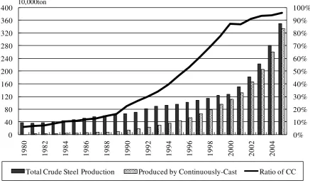
Casting processes are also important in improving energy resource efficiency. The
continuous casting share of the steel production in China increased rapidly during the 1990s,
rising from 20% in 1990 to almost 90% in 1999 (see Figure 2). Adapting modern production
processes led to productivity and energy efficiency improvements. Energy consumption per
unit of crude steel production dramatically improved when open-hearth furnaces were phased
out and the continuous casting method came into general use during the 1990s.
An increase in the water-recycling rate during the 1990s was another important
achievement resulting from technological modernization of China’s iron and steel industry. Three major factors improved water usage efficiency (China Industrial Water Conservation
Report (CIWCR), 2004). First, technological improvements in blast furnaces reduced water
usage. Second, two new drying methods for removing furnace dust required less water usage
than conventional methods and facilitated water conservation. The third factor was simplifying
production processes by installing electric arc furnaces and using the continuous casting
method. These improvements reduced the amount of water required, and the water-recycling
rate also increased because of wastewater quality improvement. The water recycling rate of
China’s iron and steel industry rose from only 57% in 1980 to 75% in 1990, and to 85% in 1999 (CIWCR). From 1990 to 1999, the volume of fresh water inputs and industrial wastewater per
ton of crude steel dropped by more than half.
Changes in policy and regulations affecting the iron and steel industry played an important
role in improving the business environment underlying the technological modernization.
China imposed price controls on steel product prices until 1992. Price deregulation affected
the performance in China’s iron and steel industry. The price of steel rapidly increased after price deregulation. Wire rod, for example, was 1,600 Yuan per ton in February 1992 before the
policy change, but immediately after the change in April 1992, the price increased to 1,750
than doubled within a year. Although the price of steel continued to increase during 1993, it
started declining in late 1993 and bottomed at 2,000 Yuan per ton in December 1993
(Yearbook of Iron and Steel Industry of China, 1994, 1995).
These rising prices enabled firms to make large profits in a short period. However, another
market reform also provided stable foundations for the iron and steel industry to ensure larger
profits during the same period. Under the contract management system, which was the sales
system introduced in the 1980s, the enterprise was permitted to sell steel products only to
customers designated by the government (Sugimoto, 1993; Ye, 2000). However, after the price
and market reforms in 1992, firms were allowed to have direct contracts with their customers.
In subsequent years, this new market system gained popularity throughout China. As a result,
the proportion of steel products sold in the new market system rapidly increased from 27% in
1988 to 91.8% in 1995 (Yearbook of Iron and Steel Industry of China, 1989, 1996).
Iron and steel firms greatly increased their profits because of increasing prices and market
reforms. These high returns encouraged technological advancements in iron and steel
production. Higher profits enabled firms to invest in new technologies such as continuous
casting equipment and basic oxygen furnaces and to build new manufacturing factories.
Additionally, the demand for high valued-added steel products, such as seamless pipe and thin
expansion, which required advanced technologies (Sugimoto, 1993). The demand push factors
further enhanced the acceleration of investments into advanced technologies.
2.2 Productivity Measurement
Many productivity evaluation techniques are based on the frontier efficiency concept
originally proposed by Farrell (1957): to evaluate inefficiency by specifying the production
frontier with the best performing observations, and measuring the distance of inefficient
samples from the frontier. The empirical specification methods of frontier efficiency divide
into two types: parametric and nonparametric. The parametric method uses Stochastic Frontier
Analysis (SFA) with production frontiers like those of the Cobb–Douglas and Translog functions (see Schmidt (1986) for survey). The nonparametric method uses the DEA developed
by Charnes et al. (1978), where nonparametric linear programming techniques are applied.
Previous studies empirically analyzing productivity in the Chinese iron and steel industry have
used both SFA and DEA.
Wu (1995) used SFA to measure the efficiency of 61 iron and steel firms in China from
1984 to 1992. Data variables are value added, fixed capital and number of workers, and the
production function was assumed to fit the Cobb–Douglas function. Wu found that productivity efficiency could increase by more than 7.0% if inefficiently performing firms
were shut down and their resources transferred to efficient firms. Movshuk (2004) measured
of value added, fixed capital, number of workers, and vintage years. He found productivity
increased at an annual rate of 6.4% using the Translog function and 4.4% using Cobb–Douglas for the period between 1988 and 2000. These two studies did not consider resource efficiency
and pollution abatement; therefore, we interpret the derived productivities as CEP. On the
other hand, Zhang et al. (2008) applied the Cobb–Douglas production function in a SFA to estimate the effects of energy-saving technologies and investments in innovation on the
productive efficiency of 19 Chinese iron and steel firms for the period from 1990 to 2000.
They found that a part of productive efficiency growth is attributable to the adoption and
amelioration of energy-saving measures (pulverized coal injection technology and continuous
casting technology). They also noted that large firms possess a substantial efficiency advantage
over small and medium steel makers.
In contrast, Ma et al. (2002) analyzed the productivity of China’s iron and steel firms by applying DEA between 1987 and 1997. They used energy consumption as an input variable in
addition to the other variables of total production value, pig iron production, crude steel
production, volume of steel products, number of workers, fixed assets, liquid assets and years
since establishment. They found that productivity improved by 3% per year.
Wei et al. (2007) investigate the energy efficiency changes in China’s iron and steel sector during the period from 1994 to 2003 using the Malmquist Index. They employed DEA model
efficiency improvement is decomposed into two components, technical change (production
frontier shifting effect), and technical efficiency change (catching-up effect) over time. The
study reported that energy efficiency in the iron and steel sector increased by 60% between
1994 and 2003. Furthermore, this increase is mainly attributable to technical progress rather
than technical efficiency improvement.
Even though many articles have already used DEA and SFA, it is not simple and easy to
expand these to consider pollution issues, partly because of the methodological difficulty
when incorporating undesirable outputs into production measurements. To address this issue,
Färe (1989) developed the Hyperbolic Distance Function (HDF), which can consistently
identify undesirable output as an extension of nonparametric approaches. However, the HDF
imposes the strong assumption of the same multiplier and divisor for increases in desirable
output and decreases in undesirable output while maintaining inputs constant. Chambers et al.
(1996) and Chung et al. (1997) developed the directional distance function (DDF) approach to
ease the restriction. There is a growing literature on methodologies for measuring productivity
efficiency with DDF incorporating environmental pollution (Hailu and Veeman, 2000; Managi
et al., 2005; Zhou, 2008; Managi et al., 2009). We examine explicitly the relative importance
of multiple environmental pollution such as both global and local pollution.
3 Methods and Data
Let 𝑥 ∈ ℜ+L, 𝑏 ∈ ℜ+R, 𝑦 ∈ ℜ+M be vectors of inputs, environmental output (or undesirable
output) and market outputs (or desirable output), respectively, and then define the production
technology as:
𝑃(𝑥) = {(𝑥, 𝑦, 𝑏): 𝑥 𝑐𝑎𝑛 𝑝𝑟𝑜𝑑𝑢𝑐𝑒 (𝑦, 𝑏)}. (1)
We assume that the good and bad outputs are null joint; a company cannot produce desirable
output without producing undesirable outputs (Shephard et al., 1974):
(𝑦, 𝑏) ∈ 𝑃(𝑥); 𝑏 = 0 ⇒ y = 0. (2)
Before defining the directional vectors in a productivity analysis that considers undesirable
outputs, either strong disposability or weak disposability needs to be assumed. The difference
between the strong and weak disposability of undesirable outputs is attributed to the
opportunity cost of pollution abatement (see Färe et al. 1986 and 1989). The strong
disposability assumes that the undesirable output is not regulated and a firm can freely
dispose it. Otherwise, regulation on the undesirable output should potentially incur the cost
for the firm to dispose. This conceptual clarification was translated into modeling framework
of frontier productivity analysis in a way that weak disposability applies when an undesirable
output is disposed of in proportion to the reduction of desirable outputs, holding the input
Considering that the pollutants in this study are CO2 emission and wastewater discharge,
CO2 emission is assumed under strong disposability and wastewater discharge is assumed
under weak disposability, respectively, since wastewater is regulated in China. Here, the
possibility that CO2 emission reduction achieved through energy and resource saving with
technological modernization, while maintaining the level of desirable outputs, is specifically
treated by setting directional vectors. If resource inputs potentially causing pollution are not
considered in the model, there is the possibility of bias in the productivity measurements
under the strong disposability assumption. Therefore, we include energy inputs in the models
and assume CO2 emission can be reduced without changing the production level of the
desirable output, but reducing energy inputs.
Weak disposability can be mathematically expressed as below (Färe et al., 1989):
(𝑦, 𝑏) ∈ 𝑃(𝑥) and 0 ≤≤ 1 ⇒ (y,b) ∈ 𝑃(𝑥). (3)
Under the null-joint hypothesis and weak disposability, this directional distance function
can be computed for firm k by solving the following optimization problem:
D⃗⃗ (x𝑘𝑙, y𝑘𝑚, b𝑘𝑟, g𝑥𝑙, g𝑦𝑚, g𝑏𝑟) = 𝑀𝑎𝑥𝑖𝑚𝑖𝑧𝑒 𝑘,
(4)
s.t. ∑𝑁𝑖=1𝜆𝑖𝑥𝑖𝑙 ≤ 𝑥𝑘𝑙 + 𝛽𝑘g𝑥𝑙 𝑙 = 1, ⋯ , 𝐿, (5)
∑𝑁𝑖=1𝜆𝑖𝑏𝑖𝑟 = 𝑏𝑘𝑟+ 𝛽𝑘g𝑏𝑟 𝑟 = 1, ⋯ , 𝑅, (7)
𝜆𝑖 ≥ 0 (𝑖 = 1, ⋯ , 𝑁), (8)
where l, m, r represent types of input, desirable output, and undesirable output, respectively. x
is an input matrix with dimensions L N, y is a desirable-output matrix with dimensions M N,
and b is an undesirable-output matrix with dimensions R N. Furthermore, gx is the directional
vector of the input matrix, gy is thedirectional vector of the desirable-output matrix and gb is
the directional vector of the undesirable-output matrix, k is the inefficiency score of the firm k,
and i is the weight variable. To estimate the inefficiency score of all firms, the model needs to
be applied independently to each of the N firms.
3.2 The Luenberger Productivity Indicator
In order to analyze changes in efficiency over time, aggregated indices such as the Malmquist
Index and Luenberger Productivity Indicator have been developed (Luenberger, 1992;
Chambers et al., 1996; Chambers, 2002). They are derived from the efficiency scores of
production frontier models. These productivity indices are measures of total factor productivity
(TFP), when the efficiency score comes from economic production frontier models. TFP
includes all categories of productivity changes and can be decomposed further to provide a
better understanding of the relative importance of various components, including Technical
production frontier, so-called frontier shift. Efficiency change measures changes in the position
of a production unit relative to the frontier, the so-called catching-up factor.
We employ the Luenberger Productivity Indicator (LPI) (Chambers et al., 1998) as a TFP
measure because the LPI is believed to be more robust than the widely used Malmquist
Indicator (Luenberger, 1992; Chambers et al., 1998). Change in the LPI is further decomposed
into technical change and efficiency change.
The Luenberger Productivity Indicator is computed with the results of the DDF model and
derived as follows (Luenberger, 1992; Chambers et al., 1998):
LPItt+1= TECHCHtt+1+ EFFCHtt+1, (9)
TECHCHtt+1= 12{D⃗⃗ t+1(𝑥
t, 𝑦t, 𝑏t) + D⃗⃗ t+1(𝑥t+1, 𝑦t+1, 𝑏t+1)
−D⃗⃗ t(𝑥
t, 𝑦t, 𝑏t) − D⃗⃗ t(𝑥t+1, 𝑦t+1, 𝑏t+1) }
, (10)
EFFCHtt+1 = D⃗⃗ t(𝑥t, 𝑦t, 𝑏t) − D⃗⃗ t+1(𝑥t+1, 𝑦t+1, 𝑏t+1), (11)
where 𝑥t represents input for year t, 𝑥t+1 is input for year t+1, 𝑦t is desirable output for year
t, and 𝑦t+1 is desirable output for year t+1. 𝑏t represents undesirable output for year t, and
𝑏t+1 is undesirable output for year t+1. The LPI score is computed based on inefficiency
scores derived from the different combinations of observations and frontiers between t and
t+1. D⃗⃗ t(𝑥t, 𝑦t, 𝑏t) denotes the inefficiency score of year t based on the frontier in year t, while
D⃗⃗ t+1(𝑥
𝐿𝑃𝐼𝑡𝑡+1+𝐿𝑃𝐼𝑡+1𝑡+2+ ⋯ + 𝐿𝑃𝐼𝑡+𝑛−1𝑡+𝑛 = 𝐿𝑃𝐼𝑡𝑡+𝑛. (12)
The DDF model commonly assumes either constant return to scale (CRS) or variable return
to scale (VRS). In this study, we apply CRS to avoid an infeasible calculation in time series
analysis. We note that imposing CRS does not eliminate the possibility of infeasible LP
problems when weak disposability is imposed on bad outputs4. When we model bad outputs in
LP, the potential for infeasible LP problems results from imposing weak disposability on the
undesirable outputs and specifying an LP problem that uses a period t reference technology
with observations from period t+15. Based on Färe (1994) and Färe et al. (1996), the VRS
model tends to have infeasible results more often than the CRS model when computing
productivity change because the VRS has stronger restrictions for solving a linear program6.
We confirmed with our models that the calculation of productivity changes under the VRS
is infeasible7. Therefore, we apply the CRS model in this study.
4 If weak disposability is imposed, the only procedure that guarantees avoiding infeasible LPs is combining a
windows technology with using only period t+1 as the reference technology for all mix-period LP problems (see
Färe et al., 2007).
5 We apply a contemporaneous frontier in our study. An alternative approach is window analysis, which is a
compromise between the contemporaneous and sequential approaches (see Shestalova, 2003; Asmild et al., 2004). Färe et al. (2001) also provided an alternative specification that combines a windows technology with using only
period t+1 as the reference technology for all mix-period LP problems to solve an infeasible LP program.
6 Färe et al. (1986) pointed out that incorporating VRS with weak disposability requires solving a nonlinear
programming problem.
7 Under VRS assumption, 41 Infeasible LP problems were found in water model, 17 infeasible LP problems
3.3 Data
Most of our dataset comes from the China Iron and Steel Industry Fifty-Year Summary
(CISIFS) and CIWCR. Data for the 27 firms covers the decade from 1990 to 1999. The
selected firms account for 68% of the crude steel production in China, based on fiscal year
2000. Mostly they are the larger firms in the industry (see Table 1). These 27 firms account for
approximately 65% of the fresh water input and industrial wastewater discharge and 45% of
total energy consumption of the iron and steel industry in 1999.
<Table 1 about here>
Profits (in real value added) and crude steel production (tonnes) are both used as the
desirable outputs, whereas fixed capital stock and gross wages are input data for productivity
estimation. Because the existence of high volatility and extreme hikes in prices of steel
products cause disturbance in, and instability of, the computation of productivity
measurements, we employ both physical outputs and value of outputs as our desirable outputs.
We admit that these two measures correlate when the price is stable. However, the correlation
does not cause problems in computation of DDF models when the price and/or value of
products are significantly changing over time in our study. However, during the 1990s, as
China’s industry strove to improve energy efficiency in crude steel production, it was also expanding into processing steel products and increasing the production of high-value-added
products, such as steel plates and steel pipes. This manufacturing process necessitates the
input of additional energy to generate the same output. Firms that followed the strategy of
developing and manufacturing high-value-added products during the 1990s may display
lower efficiency if efficiency is evaluated as the ratio of total energy consumption to crude
steel production. Therefore, developing new and high-value-added products may actually
increase energy use.
We use gross wages to reflect the quality of engineers and managers because the number of
employees or working hours does not reflect the quality of the work. We assume that the
salaries of the employees managing the modern equipment would change during the
technological modernization period.
Other variables used in the models are CO2 emissions and wastewater discharge as
undesirable outputs with energy consumption and fresh water consumption as inputs. Energy
consumption is aggregated by inputs in physical units such as electricity, coal, coke, oil, and
natural gas (CISIFS) and net calorific value coefficient (IPCC, 2006). We specially consider
double counting of the energy consumption between coal consumption and the coke-making
process (CISIFS) when the firm operates the coke-making process, and the induced energy
consumption for purchased coke otherwise. Similarly, energy for power generation is
properly treated by the national average conversion factor for electricity (China Energy
coefficients (IPCC, 2006). All monetary values of fixed capital stocks, gross wages, and value
added are deflated to fiscal year 1990 levels using the ex price indicator for the iron and steel
industry in the China Statistical Yearbook 2000.
3.4 Application of Models
This study applies the DDF to four models; namely, the Market model, the Water model, the
Energy model and the Joint model. Only the Market model has combinations of input and
output variables different from those in the other three. In the Market model, profits and
crude steel production are the desirable outputs, and capital stock and wage are the inputs. On
the other hand, in the other three models, profits and crude steel production are the desirable
outputs, and CO2 emission and wastewater discharge are the undesirable outputs.
Furthermore, energy and fresh water consumption are used as inputs in addition to capital
stock and wages. The difference between the three models is found in the directional vector
combinations as summarized in Table 28. The Water, Energy and Joint models seek to capture
environmentally sensitive productivity relating to water, energy and joint effects on water and
energy, whereas the Market model is set for reference.
<Table 2 about here>
The directional vector specifies for inefficient firms the way to improve productivity
towards the frontier production line. In the Joint, Water and Energy models, we set the
directional vector as (gy, gx, gb) = (y, –x, –b), while in the Market model, we set it as (gy, gx) = (y, –x). This type of directional vector assumes that an inefficient firm can improve productivity while increasing desirable outputs and decreasing undesirable outputs and/or
inputs in proportion to the initial combination of actual inputs and outputs.
For further analysis of the results, we separate the firms by company scale and regional
characteristics. First, we divided the sample into three groups by size of production: large,
medium and small. Companies that produced more than 5 million tons of crude steel annually
during the 1990s are categorized as large, firms with production ranging between 1 and 5
million tons as medium and firms with production of less than 1 million tons as small. The
sample sizes for large, medium and small are 4, 14 and 9 firms, respectively. Second, for
regional characteristics, we divided the sample into north and south groups by location of the
firms9. Particular attention is paid to the northern part of China, which experienced water
scarcity in the 1990s, and hence we hypothesize that firms in the north use water resources
more efficiently than those in the south. The northern group consists of 11 firms (2 large, 7
medium and 2 small) located in Beijing, Gansu, Hebei, Henan, Inner Mongolia, Jilin, Liaoning,
Shangdong and Shanxi provinces. The southern group consists of 16 firms (2 large, 7 medium
and 7 small) located in Anhui, Chongqing, Guangdong, Guizhou, Hunan, Hubei, Jiangsu,
Jiangxi, Shanghai, Sichuan, Yunnan and Zhejiang provinces.
Large and medium firms are equally located in the north and the south, but more small firms
are located in the south. Large firms started to set up continuous casting earlier than small and
medium firms in the early 1990s, but steel production in open-hearth furnaces was still
widespread even in the large firms. This can be explained by two major reasons: the rapid
increase in China’s domestic steel demand and the extremely high costs of replacing and updating equipment in large firms.
4 Results
The important results are illustrated in Figures 3 to 7 and Tables 3 and 4. The figures show the
average productivity changes derived from LPIs over the 1990s for all firms in the analysis.
The tables show the average inefficiency scores over the 1990s by size and region.
Productivity by LPIs is normalized as zero at initial productivity in 1990, while efficient
firms in the frontier line have zero in the efficiency score.
4.1 Discussion of Results for 27 Firms
Figure 3 compares the productivity changes for four models. The productivities in all models
in Figure 3 increased rapidly from 1992 to 1993, affected by the price liberalization policy in
1992. Almost all iron and steel firms experienced record profits in 1993 thanks to the price
increases. However, the productivities declined from 1993 until 1996 because steel price
decline and large investments in capital accumulation reduced capital productivity.
As the CEP in the Market model is close to zero in 1999, one can infer that market
productivity has changed little during the 1990s. The ESPs in the Water, Energy and Joint
models had trends similar to the Market model from 1990 to 1996. In contrast to the Market
model, after 1996, the ESPs gradually increased, from which it can be inferred that advances
in technology contributed to firms’ improved environmental performance. From the Joint model result, we find that water and energy efficiency improved in tandem in China’s iron and steel firms in the 1990s.
Comparison of the LPI, TECHCH, and EFFCH indicators allows us to examine how the
gaps in productivity changed. The EFFCH indicator in Figure 4 was negative in 1993 and
1994, while the TECHCH indicator in Figure 5 achieved a maximum in the same period. These
results demonstrate that the inefficient-firm group had efficiency gaps from the firms on the
frontier in 1993 and 1994 compared with 1990, but the efficiency gaps narrowed from 1994 to
1999, especially in the Water models. The EFFCH indicator in all models rose sharply after
1994, demonstrating that inefficient firms reduced their efficiency gap during this period. Most
efficient firms used continuous casting and discontinued open-hearth furnaces before 1994, but
some small and inefficient companies only introduced such equipment and process
enhancements after 1994 (CISIFS). As a result, the gap began decreasing from 1994.
<Figure 4 and Figure 5 about here>
conventional products to high-value-added products such as seamless pipe and thin steel plate
requiring more advanced technology and larger investments. Capital productivity temporarily
declined for large companies, which is consistent with the declining TECHCH indicator in the
Market model in the late 1990s. These results show the major changes in China’s production facilities during the 1990s driven by two modernization factors; namely, the rising demand for
steel products and the liberalization of the steel market.
4.2 Productivity and Firm Size
One objective of this study is to examine the differences in the efficiency gap and productivity
change among the three groups defined by firm size. From Table 3, four large firms were
efficient from 1990 to 1997 in all models even though some firms used open-hearth furnaces.
One could interpret this as the result of economies of scale. Small and medium firms improved
their efficiency from 1994 in all models, especially medium scale firms in the Water model.
These results show that the efficiency gap between efficient and inefficient firms decreased in
the 1990s.
<Table 3 and Figure 6 about here>
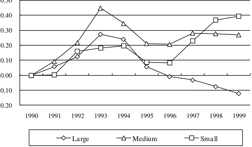
From Figure 6, medium and small firms achieved greater productivity improvements in the
1990s than large firms. The LPI of large firms from 1997 to 1999 declined in the Joint model.
Substantial investments in new equipment caused this decline, which temporarily decreased
potential to improve efficiency in the 1990s. Therefore, small firms could more easily change
production plants than large and medium firms could.
4.3 Productivity and Region
Comparing the efficiency gap by region is another objective in this study, especially because
the water shortage in northern China may affect the results in the Water model. During the
1990s, the Yellow River stopped flowing at times because of lack of water. In response, the
Yellow River Conservancy Commission of the Ministry of Water Resources restricted water
use in the industrial sector (Shao et al., 2009), forcing many firms in this region to improve
their water use efficiency to maintain production volume. Firms in the north should thus be
more water resource efficient than those in the south.
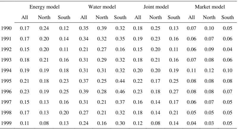
Table 4 shows the average inefficiency score by region. According to this table, northern
firms had less productive efficiency than southern firms in the early 1990s, but after 1994,
northern firms rapidly improved their efficiency in all ESP models. The Water model had
notably big regional differences between north and south. However, from Figure 7, there is
no much difference of the productivity change from 1990 to 1999 between northern firms and
southern firms. One interpretation might be that larger firms, especially Shanghai Baosteel
Group Corporation, in the south tended to introduce latest facilities from Japan and German.
Therefore, they do not require large additional investment compared to large firms in north.
addition, there are seven small firms in the south while only two in the north. Since smaller
firms often have potential productivity improvement potential, there are rather small
difference between north and south.
<Table 4 and Figure 7 about here>
5. Conclusions
This study analyzes the effect on the environmental performance of firms caused by the rapid
modernization of production facilities in the 1990s in China’s iron and steel industry. The conclusions can be summarized as follows.
First, the environmentally sensitive productivity in the Water, Energy and Joint models
shifted similarly to productivity in the Market model from 1990 to 1996. After 1996,
environmentally sensitive productivity gradually increased even as CEP decreased. From the
Joint model result, water and energy efficiency improved in tandem in Chinese iron and steel
firms in the 1990s. These results also indicate that the capital productivity of the iron and steel
sector temporarily declined in the late 1990s because of large investments in equipment
modernization. This modernization enabled steel companies to save resources and to reduce
environmental damage.
Second, the environmentally sensitive productivity of large firms was relatively low in 1999,
while that of small and medium firms improved rapidly in the 1990s. One could interpret this
firms were relatively inefficient in 1990, which provided them with potential to improve
efficiency in the 1990s.
Third, both northern and southern firms caught up to the frontier in the late 1990s. In
particular, environmentally sensitive productivity of southern firms improved more rapidly
than that of northern firms in the Water model. One could interpret this improvement as a
function of firm size distribution because the south had a higher proportion of small firms.
Small firms rapidly improved their productivity, especially in the Water model. The
environmentally sensitive productivity of northern firms improved more rapidly than that of
southern firms in the Energy model.
From a traditional viewpoint, equipment modernization is achieved by capital investment,
and this capital input decreases productivity in the short term. However, if we consider
environmental output and resource efficiency together, productivity increased even though
conventional productivity, which does not consider environmental factors, decreased in the
Chinese iron and steel sector in the 1990s. Economic and environmental concerns are
substitutes on average and on the frontier. Managers might be considering the trade-off of
resource/environmental factors and economic performance. This trade-off is evident in our
results. These aspects, especially including water usage in the data, have not been analyzed in
previous studies. Our results provide evidence to explain sustainable development by
Acknowledgements
The authors thank two anonymous referees for their helpful comments. This research was funded by
the Grant-in-Aid for Scientific Research (B) (19310023), The Ministry of Education, Culture, Sports,
Science and Technology (MEXT), Japan.
References
Asmild, M., J.C. Paradi, V. Aggarwall and C. Schaffnit (2004), ‘Combining DEA Window Analysis
with the Malmquist Index Approach in a Study of the Canadian Banking Industry’, Journal of
Productivity Analysis21: 67-89.
Asian Development Bank (2007), ‘Asian Development Outlook 2007’, Manila, Asian Development
Bank.
Chambers, R.G. (2002), ‘Exact nonradial input, output, and productivity measurement’, Economic
Theory20 (4): 751–765.
Chambers, R.G. and R.D. Pope (1996), ‘Aggregate productivity measures’, American Journal of
Agricultural Economics78 (5): 1360–1365.
Chambers, R.G., Y.H. Chung and R. Färe (1998), ‘Profit, directional distance functions, and Nerlovian
efficiency’, Journal of Optimization Theory and Applications98 (2): 351–364.
Charnes, A., C.C. Cooper and E. Rhodes (1978), ‘Measuring the efficiency of decision making units’,
European Journal of Operational Research2(6): 429–444.
China Water Power Press (2004), ‘China Industrial Water Conservation Report’, China Water Power
Press, Beijing.
China Environmental Yearbook Committee (eds) (1992–2005). ‘China Environmental Yearbook’,
China Environmental Yearbook Press, Beijing.
Chung, Y.H., R. Färe and S. Grosskopf (1997), ‘Productivity and undesirable output: A directional
distance function approach’, Journal of Environmental Management51: 229–240.
De Groot, H.L.F., C.A. Withagen and Z. Minliang (2004), ‘Dynamics of China’s regional development
and pollution: An investigation into the Environmental Kuznets Curve’, Environment and
Development Economics9: 507–537.
Färe, R., S. Grosskopf and C.A. Pasurka (1986), ‘Effects on relative efficiency in electric power
generation due to environmental controls’, Resources and Energy Economics8(2): 167–184.
Färe, R., S. Grosskopf, C.A.K. Lovell and C.A. Pasurka (1989), ‘Multilateral productivity comparisons
when some outputs are undesirable: A nonparametric approach’, The Review of Economics and
Statistics71: 90–98.
Färe, R., S. Grosskopf, M. Norris and Z. Zhang (1994), ‘Productivity growth, technical progress and
efficiency change in industrialized countries’, American Economic Review84(1): 66–83.
Färe, R., and D. Primont (1995), Multi-Output Production and Duality: Theory and Applications,
Kluwer Academic Publishers, Boston.
Färe, R., S. Grosskopf and C.A. Pasurka (2001), ‘Accounting for air pollution emissions in measures
of state manufacturing productivity growth’, Journal of Regional Science41(3): 381–409. Färe, R., S. Grosskopf and C. Pasurka (2007), ‘Pollution abatement activities and traditional
productivity’, Ecological Economics62(3-4): 673–682.
Farrell, M.J. (1957), ‘The measurement of productive efficiency’, Journal of the Royal Statistical
Society. Series A (General) 120(3): 253–290.
Fisher-Vanden, K., G. Jefferson, H. Liu and Q. Tao (2004), ‘What is driving China’s decline in energy
intensity? ’, Resource and Energy Economics26(1): 77–97.
Hailu, A. and T.S. Veeman (2000), ‘Environmentally sensitive productivity analysis of the Canadian pulp and paper industry, 1959–1994: An input distance function approach’, Journal of
Environmental Economics and Management 40: 251–274.
Intergovernmental Panel on Climate Change (IPCC) (2006), ‘2006 IPCC Guidelines for National
Greenhouse Gas Inventories: Volume 1 General Guidance and Reporting’, IPCC, Japan.
International Iron and Steel Institute (2005a) ‘Steel Statistical Yearbook 2005’, International Iron and
Steel Institute, Brussels.
International Iron and Steel Institute (2005b), ‘World Steel in Figures 2005’, International Iron and
Steel Institute, Brussels.
Jiang, T. and W.J. McKibbin (2002), ‘Assessment of China’s pollution levy system: An equilibrium
pollution approach’, Environment and Development Economics7: 75–105.
Kim, Y. and E. Worrell (2002), ‘International comparison of CO2 emission trends in the iron and steel
industry’, Energy Policy30: 827–838.
Kaneko, S., A. Yonamine and T.Y. Jung (2006), ‘Technology choice and CDM projects in China: Case
study of a small steel company in Shandong province’, Energy Policy34(10): 1139–1151. Luenberger, D.G. (1992), ‘Benefit function and duality’, Journal of Mathematical Economics
21:461–481.
Ma, J., D.G. Evans, R.J. Fuller and D.G. Stewart (2002), ‘Technical efficiency and productivity change
of China’s iron and steel industry’, International Journal of Production Economics76: 293–312.
Managi, S. and S. Kaneko (2009), 'Environmental performance and returns to pollution abatement in
China', Ecological Economics68(6): 1643-1651.
Managi, S., J.J. Opaluch, D. Jin and T.A. Grigalunas (2005) ‘Environmental Regulations and Technological Change in the Offshore Oil and Gas Industry’, Land Economics81(2): 303-319. Ministry of Metallurgical Industry (2003), ‘China Iron and Steel Industry Fifty-Year Summary
(Volumes 1 and 2)’, Metallurgical Industry Press, Beijing.
Ministry of Metallurgical Industry (eds) (1989–2003), ‘Yearbook of Iron and Steel Industry of China’,
Metallurgical Industry Press, Beijing.
Movshuk, O. (2004), ‘Restructuring, productivity and technical efficiency in China’s iron and steel
industry, 1988–2000’, Journal of Asian Economics15: 135–151.
Schmidt, P. (1986), ‘Frontier production functions’, Econometric Reviews4: 289–328.
Shao, W., D. Yang, H. Hu and K. Sanbongi (2009), ‘Water resources allocation considering the water
use flexible limit to water shortage—A case study in the Yellow River Basin of China’, Water
Resources Management23(5): 869–880.
Shephard, R.W. and R. Färe (1974), ‘The law of diminishing returns’, Journal of Economics 34(1):
69–90.
Shestalova, V (2003),’Sequential Malmquist Indices of Productivity Growth: An Application to OECD Industrial Activities’, Journal of Productivity Analysis19: 211-226.
State Statistical Bureau (eds) (1991–1996, 1997–1999, 2005). ‘China Energy Statistical Yearbook’,
China Statistical Press, Beijing.
State Statistical Bureau (eds) (1986–2006). ‘China Statistical Yearbook’, China Statistical Press,
Beijing.
Sugimoto, T. (1993), ‘The Chinese steel industry’, Resource Policy19(4): 264–286.
Vardanyan, M. and D.-W. Noh (2006), ‘Approximating pollution abatement costs via alternative
specifications of a multi-output production technology: A case of the US electric utility industry’,
Journal of Environmental Management, 80, No. 2 (July), 177–190.
Wang, H. and D. Wheeler (2003), ‘Equilibrium pollution and economic development in China’,
Environment and Development Economics8: 451–466.
Woo, W. T. (2007), ‘What are the high-probability challenges to continued high growth in China?’
Working Paper, The Brookings Institution, Washington, DC.
Wu, Y. (1995), ‘The productive efficiency of Chinese iron and steel firms: A stochastic frontier
analysis’, Resource Policy21: 215–222.
World Bank (2007), ‘Cost of Pollution in China: Economic Estimates of Physical Damages’, World
Bank, Washington, DC.
World Bank (2008), ‘Water Supply Pricing in China: Economic Efficiency, Environment, and Social Affordability’, World Bank, Washington, DC.
Worrell, E., L. Price, N. Martin, J. Farla and R. Schaeffer (1997), ‘Energy intensity in the iron and steel
industry: A comparison of physical and economic indicators’, Energy Policy25: 727–744.
Ye, G. (2000), The Growth of Iron and Steel Industry in China, Yotsuya Round Publishers, Tokyo. Wei, Y.M., H. Liao and Y. Fan (2007), ‘An empirical analysis of energy efficiency in China’s iron and
steel sector’, Energy32(12): 2262–2270.
Zhang, Y. (2002), ‘The impacts of economic reform on the efficiency of silviculture: A non-parametric
approach’, Environment and Development Economics7: 107–122.
Zhang, J. and Wang, G. (2008), ‘Energy saving technology and productivity efficiency in the Chinese
iron and steel sector’, Energy33(4): 525–537.
Zhou, P., B.W. Ang and K.L. Poh (2008), ‘A survey of data envelopment analysis in energy and
Table 1 Size breakdown of firms in China’s iron and steel industry
Total crude steel production
(million tons)
Number of iron and steel firms
Overall China Samples in this study
In 1990:
0.50 to 0.99 12 9
1.00 to 4.99 16 12
5.00 or greater 0 0
Total numbers of firms 1,589 27
In 2000:
0.50 to 0.99 13 0
1.00 to 4.99 37 23
5.00 or greater 4 4
Total numbers of firms 2,997 27
Source: Yearbook of Iron and Steel Industry of China 2003
Table 2 Combinations of directional vector in each model for calculating inefficiency of firm k
Water model Energy model Joint model Market model
Directional vector of
desirable output (gy)
Crude steel 𝑦𝑘𝑠𝑡𝑒𝑒𝑙 𝑦𝑘𝑠𝑡𝑒𝑒𝑙 𝑦𝑘𝑠𝑡𝑒𝑒𝑙 𝑦𝑘𝑠𝑡𝑒𝑒𝑙
Value added 𝑦𝑘𝑣𝑎𝑙𝑢𝑒 𝑦𝑘𝑣𝑎𝑙𝑢𝑒 𝑦𝑘𝑣𝑎𝑙𝑢𝑒 𝑦𝑘𝑣𝑎𝑙𝑢𝑒
Directional vector of
undesirable output (gb)
Waste water 𝑏𝑘𝑤𝑎𝑠𝑡𝑒 0 𝑏𝑘𝑤𝑎𝑠𝑡𝑒 Unused
CO2 0 𝑏
𝑘
𝐶𝑂2 𝑏
𝑘
𝐶𝑂2 Unused
Directional vector of
input (gx)
Labor 0 0 0 𝑥𝑘𝑙𝑎𝑏𝑜𝑟
Capital stock 0 0 0 𝑥𝑘𝑐𝑎𝑝𝑖𝑡𝑎𝑙
Fresh water 𝑥 𝑘
𝑓𝑟𝑒𝑠ℎ 0 𝑥
𝑘
𝑓𝑟𝑒𝑠ℎ Unused
Energy 0 𝑥𝑘𝑒𝑛𝑒𝑟𝑔𝑦 𝑥𝑘𝑒𝑛𝑒𝑟𝑔𝑦 Unused
Note: All of these variables are used as data in three ESP models. The nonzero value indicates the variable is
also used as directional vector. The value of zero indicates that the variable is not used as a directional vector but
[image:32.595.91.506.412.584.2]Table 3 Average inefficiency score by company scale
Energy model Water model Joint model Market model
Large Medium Small Large Medium Small Large Medium Small Large Medium Small
1990 0.00 0.25 0.14 0.00 0.47 0.35 0.00 0.27 0.15 0.00 0.06 0.11
1991 0.01 0.19 0.16 0.02 0.39 0.39 0.01 0.20 0.21 0.00 0.05 0.12
1992 0.00 0.17 0.16 0.00 0.21 0.29 0.00 0.16 0.17 0.00 0.05 0.12
1993 0.00 0.15 0.35 0.00 0.26 0.59 0.00 0.13 0.36 0.00 0.06 0.11
1994 0.00 0.15 0.30 0.00 0.22 0.61 0.00 0.15 0.34 0.00 0.12 0.14
1995 0.00 0.18 0.34 0.00 0.29 0.66 0.00 0.17 0.38 0.00 0.08 0.12
1996 0.00 0.19 0.35 0.00 0.31 0.69 0.00 0.19 0.39 0.00 0.08 0.11
1997 0.00 0.15 0.24 0.00 0.26 0.58 0.00 0.15 0.26 0.00 0.07 0.07
1998 0.01 0.15 0.24 0.01 0.24 0.42 0.01 0.16 0.26 0.02 0.05 0.07
1999 0.00 0.08 0.17 0.00 0.15 0.49 0.00 0.08 0.19 0.03 0.05 0.03
Table 4 Average inefficiency score in 27 firms, North and South group
Energy model Water model Joint model Market model
All North South All North South All North South All North South
1990 0.17 0.24 0.12 0.35 0.39 0.32 0.18 0.25 0.13 0.07 0.10 0.05
1991 0.17 0.20 0.14 0.34 0.32 0.35 0.19 0.23 0.16 0.06 0.07 0.06
1992 0.15 0.20 0.11 0.21 0.27 0.16 0.15 0.20 0.11 0.06 0.09 0.04
1993 0.18 0.21 0.16 0.31 0.29 0.32 0.18 0.21 0.16 0.07 0.08 0.06
1994 0.19 0.19 0.18 0.31 0.31 0.32 0.20 0.20 0.19 0.11 0.12 0.10
1995 0.21 0.18 0.23 0.37 0.25 0.44 0.22 0.17 0.25 0.08 0.08 0.08
1996 0.23 0.19 0.25 0.39 0.28 0.46 0.23 0.18 0.27 0.08 0.08 0.07
1997 0.15 0.13 0.16 0.31 0.21 0.37 0.16 0.14 0.17 0.06 0.07 0.05
1998 0.17 0.13 0.20 0.27 0.21 0.32 0.18 0.14 0.21 0.05 0.05 0.05
[image:33.595.100.501.418.635.2]Figure 1 Share of steel production by operation method
Source: Steel Statistical Yearbook 2005 (International Iron and Steel Institute, 2005a)
Figure 2 Crude steel production and continuous casting ratio
0% 10% 20% 30% 40% 50% 60% 70% 80% 90% 100%
1980 1982 1984 1986 1988 1990 1992 1994 1996 1998 2000 2002 2004
Oxygen Blown Converters Electric Furnaces Open Hearth Furnaces
0% 10% 20% 30% 40% 50% 60% 70% 80% 90% 100% 0 40 80 120 160 200 240 280 320 360 400
1980 1982 1984 1986 1988 1990 1992 1994 1996 1998 2000 2002 2004
Total Crude Steel Production Produced by Continuously-Cast Ratio of CC
[image:34.595.83.521.464.722.2]Figure 3 27 firms’ average score of cumulative productivity (LPI) change in each model
Figure 4 27 firms’ average score of cumulative efficiency change (EFFCH) in each model -0.10
0.00 0.10 0.20 0.30 0.40 0.50 0.60
1990 1991 1992 1993 1994 1995 1996 1997 1998 1999
Energy Wa ter Joint Ma rket
-0.10 -0.05 0.00 0.05 0.10 0.15 0.20
1990 1991 1992 1993 1994 1995 1996 1997 1998 1999
[image:35.595.83.517.488.761.2]Figure 5 27 firms’ average score of cumulative technical change (TECHCH) in each model
Figure 6 Cumulative productivity (LPI) score in Joint model by firm scale 0.00
0.10 0.20 0.30 0.40 0.50
1990 1991 1992 1993 1994 1995 1996 1997 1998 1999
Energy Wa ter Joint Ma rket
-0.20 -0.10 0.00 0.10 0.20 0.30 0.40 0.50
1990 1991 1992 1993 1994 1995 1996 1997 1998 1999
[image:36.595.88.511.492.738.2]Figure 7 Cumulative productivity (LPI) score in Joint model by region
0.00 0.05 0.10 0.15 0.20 0.25 0.30 0.35 0.40
1990 1991 1992 1993 1994 1995 1996 1997 1998 1999