Merits and drawbacks of variance targeting in GARCH models

Munich Personal RePEc Archive

Merits and drawbacks of variance

targeting in GARCH models

Francq, Christian and Horvath, Lajos and Zakoian,

Jean-Michel

Université Lille III, GREMARS-EQUIPPE, University of Utah,

Department of Mathematics, GREMARS-EQUIPPE and CREST

2009

Online at

https://mpra.ub.uni-muenchen.de/15143/

Merits and drawbacks of variance targeting in GARCH models

Christian Francq

∗

_{, Lajos Horvath}

†

_{and Jean-Michel Zakoïan}

‡

May 3, 2009

Variance targeting estimation is a technique used to alleviate the numerical difficulties en-countered in the quasi-maximum likelihood (QML) estimation of GARCH models. It relies on a reparameterization of the model and a first-step estimation of the unconditional variance. The remaining parameters are estimated by QML in a second step. This paper establishes the asymptotic distribution of the estimators obtained by this method in univariate GARCH mod-els. Comparisons with the standard QML are provided and the merits of the variance targeting method are discussed. In particular, it is shown that when the model is misspecified, the VTE can be superior to the QMLE for long-term prediction or Value-at-Risk calculation. An empir-ical application based on stock market indices is proposed.

Keywords.

Consistency and Asymptotic Normality, GARCH, Heteroskedastic Time Series, Quasi

Maximum Likelihood Estimation, Value-at-Risk, Variance Targeting Estimator.

1

Introduction

More than two decades after the introduction of ARCH models and their generalization (Engle (1982), Bollerslev (1986)), the properties of GARCH type sequences are well understood and general statistical methods have been established to work with this type of sequences. In recent years, special attention has been given to the asymptotic properties of the Gaussian quasi-maximum likelihood estimation (QMLE) (see Berkes, Horváth, and Kokoszka (2003), Francq and Zakoïan (2004), and the recent monograph by Straumann (2005), among others). While many other estimation methods have been proposed for GARCH-type models (for instance theLp-estimators of Horváth and Liese (2004), the self-weighted QMLE of Ling (2007)), QMLE can be recommended for at least two reasons: i) it is consistent under very mild conditions, in particular it is robust to the distribution of the underlying iid process, and ii) no moment condition has to be imposed on the observations to obtain consistency and asymptotic normality.

However, practitioners are often reluctant to directly apply the QMLE to their data. They generally make use of closed-form estimators to reduce the dimensionality of the parameter space, or to speed-up the convergence of the optimization routines. Such estimators are particularly attractive for the estimation of multivariate GARCH models, or when a large number of univariate GARCH models have to be estimated (see Bauwens and Rombouts (2007)). In the framework of a scalar BEKK (Engle and Kroner (1995)), Engle and Mezrich (1996) proposed a two-step estimation method, the so-called variance targeting estimation

∗

Université Lille III, GREMARS-EQUIPPE Universités de Lille, BP 60149, 59653 Villeneuve d’Ascq cedex, France. E-Mail: [email protected]

†_{University of Utah, Department of Mathematics, 155 South 1400 East, Salt Lake City UT 84112-0090, USA.}

E-mail: [email protected]

‡_{GREMARS-EQUIPPE and CREST, 15 boulevard Gabriel Péri, 92245 Malakoff Cedex, France. E-mail:}

(VTE) method. The method is based on a reparamerization of the volatility equation, in which the intercept is replaced by the returns unconditional variance (the long-run variance). A first-step estimator of the unconditional variance is computed while, conditioning on this estimate, the remaining parameters are estimated by QML in a second step.

To our knowledge, the asymptotic properties of the VTE have not been established, and they are the main aim of this paper. While the VTE method facilitates the estimation of parameters in GARCH models, even in the simple univariate GARCH(1,1), it is not clear if this advantage is not paid for in terms of asymptotic accuracy loss, when the VTE is compared to the QMLE. Intuitively, even if the sample variance converges to the population variance, the use of a two-step procedure should deteriorate the asymptotic precision of the GARCH QML estimates for Gaussian iid errors. The magnitude of the accuracy loss, however, cannot be intuited. Moreover, for non Gaussian iid errors, the superiority of QMLE over the VTE cannot be taken for granted.

On the other hand, the potential merits of the VTE may not be limited to numerical simplicity. This procedure guarantees that the estimated unconditional variance of the GARCH model is equal to the sample variance. It is therefore possible that, in case of misspecification,i.e. when the true underlying process is not a GARCH, the GARCH approximation provided by the VTE is superior, in some sense, to that obtained by QMLE. This issue will be examined through the problems of long-term prediction and Value-at-Risk (VaR) calculation.

The VTE is a two-step estimator, the marginal variance being estimated in a first step and then plugged in the quasi-likelihood in a second step. Two-step estimators are quite common in econometrics but, in general, these estimators are given in closed form. From a technical point of view, the main difficulty here is that the first step estimator is plugged in a criterion, not directly in a formula giving the second-step estimator. This particularity makes the proof of the asymptotic properties of the VTE non standard.

The paper is organized as follows. Section 2 describes the reparameterization of the standard GARCH(1,1) model and provides the asymptotic properties of the VTE. Section 3 proposes an extension to the GARCH(p, q) model. Section 4 examines the performances of the VTE, by comparison to the QMLE, in the cases of well-specified and miswell-specified models. An empirical comparison based on eleven stock indices is also proposed. Section 5 concludes and outlines topics for future research. Proofs are relegated to an appendix.

2

Asymptotic distribution of the VTE in the GARCH(1,1) case

Consider the GARCH(1,1) model

ǫt=√htηt

ht=ω0+α0ǫ2t−1+β0ht−1, ∀t∈Z (2.1) whereθ0= (ω0, α0, β0)′ is an unknown parameter,

(ηt)is a sequence of independent and identically distributed (i.i.d) random variables (2.2)

such that

Eη2t = 1, (2.3)

and

ω0>0, α0≥0, β0≥0. (2.4)

Under the condition

α0+β0<1 (2.5)

this model admits a second-order stationary solution(ǫt), whose unconditional variance is given by

γ0:=σ2(ω0, α0, β0) = ω0

1₋α0−β0

:=ω0

κ0 .

A reparametrization of the model withϑ0= (γ0, α0, κ0)′ yields

ǫt=

p

which allows us to interpretκ0as the speed of mean reversion in variance (see Christoffersen (2008)). Writing

ht=κ0γ0+α0ǫ2t−1+β0ht−1, κ0+α0+β0= 1,

one can also interpret the volatility at timet,ht, as a weighted average of the long-run varianceγ0, of the square of the last returnǫ2

t−1 and of the previous volatility ht−1. In this average, κ0 is the weight of the long-run variance. Note that in this reparametrization, constraints (2.4) and (2.5) become

κ0, γ0>0, α0≥0, κ0+α0≤1. (2.7)

Let(ǫ1, . . . , ǫn)be a realization of lengthnof the unique nonanticipative second-order stationary solution (ǫt)to model (2.1) which satisfies (2.3) and (2.7). In this framework, VTE involves (i) reparametrizing the model as in (2.6), (ii) estimatingγ0by the sample variance and thenλ0:= (α0, κ0)′ by the QML estimator.

The QMLE of θ0 is denoted by ˆθ

∗

n := (ˆωn∗,αˆ∗n,βˆn∗)′. Two consistent estimators of γ0 are the sample

variance and the QML-based estimator, given by

ˆ σ2

n = 1 n

n

X

t=1 ǫ2

t, and σ2(ˆθ

∗

n) = ˆ ω∗

n

1₋αˆ∗

n−βˆn∗ .

Horváth, Kokoszka and Zitikis (2006) showed that the differenceσˆ2

n−γ0andσˆ2n−σ2(ˆθ

∗

n)are asymptotically normal, with different asymptotic variances. They also use the latter difference as a statistic for testing that the model is correctly specified.

Consider a parameter space Λ ⊂ {(α, κ) | α ≥ 0, κ > 0, α+κ ≤ 1}. Set λ0 = (α0, κ0)′ and write

λ= (α, κ)′ _{and β = 1−α−κ. At this stage, we use the convention that all the vectors considered in the}

sequel are column vectors even when, for simplicity, they are written as row vectors. In particular we write

ϑ0= (γ0,λ0)instead ofϑ0= (γ0,λ′0)′. At the pointϑ= (γ,λ)∈(0,∞)×Λ, the Gaussian quasi-likelihood of the sample is given by

˜

Ln(ϑ) = ˜Ln(γ,λ) =

n

Y

t=1 1

p

2π˜σ2

t(ϑ) exp

− ǫ 2 t

2˜σ2

t(ϑ)

,

where the˜σ2

t(ϑ)’s are defined recursively, fort≥1, by

˜

σ2t(ϑ) =κγ+αǫ2t−1+ (1−κ−α)˜σt2−1(ϑ) (2.8)

with the initial valuesǫ0and σ˜02(ϑ) :=σ02. Since the parameterγ0 is estimated by the sample varianceˆσn2, the variance targeting version of the Gaussian quasi-likelihood function is

Ln(λ) = ˜Ln(ˆσ2

n,λ) = n

Y

t=1 1

q

2πσ2

t,n exp

− ǫ 2 t

2σ2

t,n

,

where

σt,n2 :=σt,n2 (λ) =κσˆn2+αǫ2t−1+ (1−κ−α)σt2−1,n

withσ2

0,n=σ02.A variance targeting estimator (VTE) ofλ0 is defined as any measurable solutionλˆn of ˆ

λn=arg max

λ_∈Λ

Ln(λ) =arg min

λ_∈Λ

˜_{ln(λ). (2.9)}

where

˜_{ln(λ) =n}−1

n

X

t=1

ℓt,n, and ℓt,n:=ℓt,n(λ) = ǫ 2 t σ2 t,n

+ logσt,n2 . (2.10)

Note thatσ2

t,n = ˜σt2(ˆσ2n,λ). For anyϑ= (γ,λ)∈(0,∞)×Λwe have0≤1−κ−α <1, and one can define

the strictly stationary and ergodic process

σ2

t(ϑ) =κγ+αǫ2t−1+ (1−κ−α)σt2−1(ϑ) =

∞

X

i=0

(1₋κ₋α)i_(κγ+αǫ2

Note thatht=σt2(γ0,λ0). We denote byϑˆn= (ˆσn2,λˆn)the VTE ofϑ0.

To show the strong consistency and the asymptotic normality of the VTE, the following assumptions will be made.

A1: λ0belongs toΛand Λis compact.

A2: ηt2has a non-degenerate distribution.

A3: α20 Eη4t−1

+ (1−κ0)2<1.

A4: λ0belongs to the interior of Λ.

Note thatA3is the necessary and sufficient condition forEǫ4 t <∞.

Theorem 2.1 Under assumptionsA1-A2,α06= 0, and (2.2)–(2.5), the VTE satisfies

ˆ

ϑn →ϑ0,

almost surely as n_{→ ∞}and, under the additional assumptions A3-A4, we have

√

nϑˆn−ϑ0

_d

→ N(0,(Eη40−1)Σ), where the matrix

Σ=

b −bK′J−1

−bJ−1K J−1+bJ−1KK′J−1

is non-singular with

b= (α0+κ0) 2

κ2 0

E(h2 t) =

(α0+κ0)2γ2(2−κ0)

κ0{1−α20(Eηt4−1)−(1−κ0)2} and

J =E

₁

σ4 t(ϑ0)

∂σ2 t(ϑ0) ∂λ

∂σ2 t(ϑ0) ∂λ′

2×2

, K=E

₁

σ4 t(ϑ0)

∂σ2 t(ϑ0) ∂λ

∂σ2 t(ϑ0) ∂γ

2×1

. (2.12)

This result complements the paper of Horváth, Kokoszka and Zitikis (2006), where the asymptotic distribu-tion of√n(ˆσ2

n−γ0)was derived. Lettingλˆn= (ˆλ1n,λˆ2n), the VTE of the original parameterθ0= (ω0, α0, β0) is defined byθˆn = (ˆωn,αˆn,βˆn) whereωˆn = ˆλ2nσˆn2, αˆn = ˆλ1n, βˆn = 1−ˆλ1n−λˆ2n. Theorem 2.1 yields the following result.

Corollary 2.1 Under the assumptions of Theorem 2.1, the VTE of θ0 satisfies

√

nθˆn−θ0

_d

→ N(0,(Eη04−1)L′ΣL), L=



 1−α00−β0 01 −01 ω0(1−α0−β0)−1 0 −1

 .

It is important to note that the asymptotic normality of the VTE requires the existence ofE(ǫ4t), whereas the strict stationarity is sufficient for the asymptotic normality of the QMLE (see Berkes, Horváth and Kokoszka (2003) and Francq and Zakoïan (2004)). The QMLE ofϑ0is denoted byϑˆ

∗

n = (ˆγn∗,αˆ∗n,κˆ∗n). The asymptotic

variance matrix ofϑˆ∗n is(Eη04−1)Σ∗where

(Σ∗)−1=E

₁

σ4 t(ϑ0)

∂σ2 t(ϑ0) ∂ϑ

∂σ2 t(ϑ0) ∂ϑ′

=

κ2 0

(α0+κ0)2E(1/h

2 t) K′

K J

!

.

Corollary 2.2 Under the assumptions of Theorem 2.1, the asymptotic variance (Eη4

0−1)Σ of the VTE and the asymptotic variance (Eη4

0−1)Σ∗ of the QMLE of ϑ0 satisfy

Σ−Σ∗= (b−a)CC′, where

C=

1 −J−1K

, a=

_κ2 0

(α0+κ0)2

E(1/h2 t)−K

′

J−1K −1

.

Note that a >0 because detΣ∗ =adetJ−1. It will be shown that b₋a _≥0 (in a more general setting, see Proposition 3.1 below), which implies that the VTE cannot be asymptotically more accurate than the QMLE. Corollary 2.2 shows that, as expected, the VTE becomes much less accurate than the QMLE when α2

0 Eη4t−1

+ (1₋κ0)2 _{approaches 1. More interestingly, the relative loss of efficiency of the VTE is the} same for all 3 parameters γ0, α0 and κ0. In general the asymptotic variances of the GARCH coefficients which are estimated by the two methods do not coincide. This point will be illustrated in Section 4.

3

Extension to the general GARCH(

p, q

) case

In this section we consider the general GARCH(p, q) model

ǫt=√htηt

ht=ω0+P_i=1q α0iǫ2t−i+

Pp

j=1β0jht−j, ∀t∈Z

(3.1)

where(ηt)satisfies (2.2)-(2.3) and where the coefficients satisfy:

ω0>0, α0i≥0 ∀i∈ {1, . . . , q}, β0j≥0 ∀j∈ {1, . . . , p}. (3.2)

Under the condition

q

X

i=1 α0i+

p

X

j=1

β0j <1. (3.3)

the observations have finite varianceγ0=ω0

n

1−Pqi=1α0i−Ppj=1β0j

o−1

.In this section we parameterize the model with

ϑ0= (γ0, α01, . . . , α0q, β01, . . . , β0p) = (γ0,λ0)∈(0,∞)×Λ,

whereΛis included in the simplex nλ= (λ1, . . . , λp+q) : λi≥0∀i∈ {1, . . . , p+q}, Pp+q_i=1λi<1

o

.

The VTE ofϑ0 isϑˆn = (ˆσ2n,λˆn), where σˆn2 =n−1P n t=1ǫ2t,

ˆ

λn=arg min

λ_∈Λ

˜_ln(λ), ˜_{ln(λ) =n}−1

n

X

t=1 ˜

ℓt(ˆσ2n,λ), ℓ˜t(ϑ) = ǫ2

t ˜ σ2

t(ϑ)

+ log ˜σt2(ϑ),

and theσ˜2

t(ϑ)’s are defined recursively, fort≥1, by

˜

σ2t(ϑ) = ˜σt2(γ,λ) =γ 1−

p+q

X

i=1 λi

!

+ q

X

i=1

λiǫ2t−i+ p

X

j=1

λq+jσ˜t2−j(ϑ)

with fixed initial values for ǫ0, . . . , ǫ1−q and σ˜02(ϑ), . . . ,σ˜12−p(ϑ). Define Aϑ(z) = P_i=1q λ_izi andBϑ(z) =

1−Ppj=1λq+jzj, with the conventionAϑ(z) = 0 if q= 0 and Bϑ(z) = 1 ifp= 0. We need the following

additional identifiability assumption:

A5: ifp >0,Aϑ0(z)andBϑ0(z)have no common root,Aϑ0(1)6= 0, andα0q+β0p6= 0.

Theorem 3.1 Under assumptionsA1with (3.2) and (3.3),A2with (2.2) and (2.3), andA5, the VTE of the GARCH(p, q)model (3.1) is strongly consistent. Under the additional assumptions Eǫ4

t <∞ andA4,

we have _√

nϑˆn−ϑ0

_d

→ N0,(Eη04−1)Σ , (3.4) where the matrix

Σ=

c ₋cK′J−1

−cJ−1K J−1+cJ−1KK′J−1

is non-singular with

c= 1−

Pq i=1β0i

1−Pqi=1α0i−

Pp j=1β0j

!2 E(h2

t)

and

J =E

₁

σ4 t(ϑ0)

∂σ2 t(ϑ0) ∂λ

∂σ2 t(ϑ0) ∂λ′

(p+q)×(p+q)

, K=E

₁

σ4 t(ϑ0)

∂σ2 t(ϑ0) ∂λ

∂σ2 t(ϑ0) ∂γ

(p+q)×1 .

Under these assumptions, the QMLEϑˆ∗n satisfies √_nˆ

ϑ∗n−ϑ0

_d

→ N0,(Eη4

0−1)Σ∗ , (3.5) where

Σ∗=Σ−(c−d)CC′, (3.6) with

C =

₁

−J−1K

, d=

  

1₋Pq_i=1α0i−Ppj=1β0j

1₋Pq_i=1β0i

!2 E

₁

h2 t

−K′J−1K   

−1

.

The following result shows that the VTE can never be asymptotically more efficient than the QMLE, re-gardless of the values of the GARCH parameters and the distribution ofηt.

Proposition 3.1 Under the assumptions of Theorem 3.1, the asymptotic variance(Eη4

0−1)Σof the VTE and the asymptotic variance (Eη4

0−1)Σ

∗ _{of the QMLE satisfy}

Σ−Σ∗ is positive semidefinite, but not positive definite.

The following result characterizes the parameters that are estimated with the same asymptotic accuracy by the VTE and by the QMLE.

Corollary 3.1 Let the assumptions of Theorem 3.1 be satisfied, and let φbe a mapping fromRp+q+1 _toR_,

which is continuously differentiable in a neighborhood ofϑ0. If

∂φ

∂ϑ′(ϑ0)

1 −K′J−1

= 0,

then the asymptotic distribution of the VTE of the parameter φ(ϑ0) is the same as that of the QMLE, in the sense that

√

nnφ(ˆϑn)−φ(ϑ0)o→ Nd 0, s2, √nnφ(ˆϑ∗_n)−φ(ϑ0)o→ Nd 0, s2,

where

s2= (Eη40−1) ∂φ

∂ϑ′Σ

∂φ

4

Comparisons with the QMLE

In this section we compare the effective performance of the QMLE and VTE. In the first subsection, we numerically evaluate and compare the asymptotic variances of the two estimators. For simplicity, this comparison is made in ARCH(1) models. The second subsection presents simulation results with the aim to determine whether the ratio of the asymptotic variances gives a good idea of the ratio of accuracies of the two estimators in finite samples. Subsection 4.3 studies the estimation of the parameters of a set of typical financial time series using both methods. Subsection 4.4 considers the situation where the GARCH model is misspecified. It will be shown that the fact that the VTE guarantees a consistent estimation of the long-run variance may be a crucial advantage of the VTE over the QMLE.

4.1

Asymptotic variances of the QMLE and VTE for ARCH(1) models

For an ARCH(1) model, the asymptotic variancesΣandΣ∗of the VTE and QMLE are given by Theorem 3.1 with

c= 1

(1₋α0)2Eh

2

t, J =E

_(ǫ2

t−1−γ0)2 h2

t

, K= (1₋α0)E

_ǫ2 t−1−γ0

h2 t

.

In particular, the asymptotic variance of the VTEαˆn ofα0 is given by

lim n→∞Var{

√

n(ˆαn−α0)}=

Eη4 0−1 E(ǫ2

t−1−γ0)2/σt4

"

1 + Eσ

4 t E

(ǫ2

t−1−γ0)/σ4t 2

E(ǫ2

t−1−γ0)2/σt4

#

.

For the QMLEαˆ∗

n ofα0 the asymptotic variance is

lim n→∞Var{

√

n(ˆα∗n−α0)}=

Eη4 0−1 E(ǫ2

t−1−γ0)2/σ4t

"

1 + E

(ǫ2

t−1−γ0)/σt4 2

E(1/σ4 t)E

(ǫ2

t−1−γ0)2/σt4 − E

(ǫ2

t−1−γ0)/σt4 2

#

= (Eη

4

0−1)E 1/σ4t

E(1/σ4

t)E ǫ4t−1/σ4t

−E ǫ2 t−1/σ4t

2,

where the first equality is obtained with the parametrization ϑ0 = (γ0, α0), and the second equality with the parametrizationθ0= (ω0, α0).

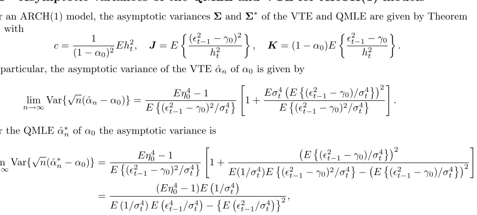
The results presented in Table 1 are obtained from simulations of the matricesΣ and Σ∗ above, with expectations replaced by empirical means. More precisely, the table displays the mean of 1,000 independent estimates of the matrices

2Σ= lim

n→∞Var{

√

n(ˆϑn−ϑ0)} and 2Σ∗= lim

n→∞Var{

√

n(ˆϑ∗n−ϑ∗0)},

[image:8.612.70.535.174.384.2]

where each estimation is obtained from empirical means based on a simulation of size n = 10,000 of the ARCH(1) model. It is seen that the variance targeting does not affect the asymptotic distribution of the estimator of ϑ0 when α0 is small, but entails a dramatic loss of efficiency when α0 approaches the limit implied by the existence of a fourth moment (α0<0.57whenηt has a standard normal distribution).

Table 2 is the analog of Table 1, but gives the asymptotic variances of the QMLE and VTE for the standard ARCH parameterθ0= (ω0, α0). From this table, it is seen that the asymptotic distribution of the VTE of the parameterω0should be close to that of the QMLE. This is not surprising because we know from Corollary 3.1 that there exist transformations ofϑ0 which are estimated by VTE and QMLE with the same asymptotic accuracy.

4.2

Sampling distribution of the QMLE and VTE

is not satisfied, so the asymptotic normality of the VTE is not guaranteed. Table 3 provides an overview of these simulations experiments.

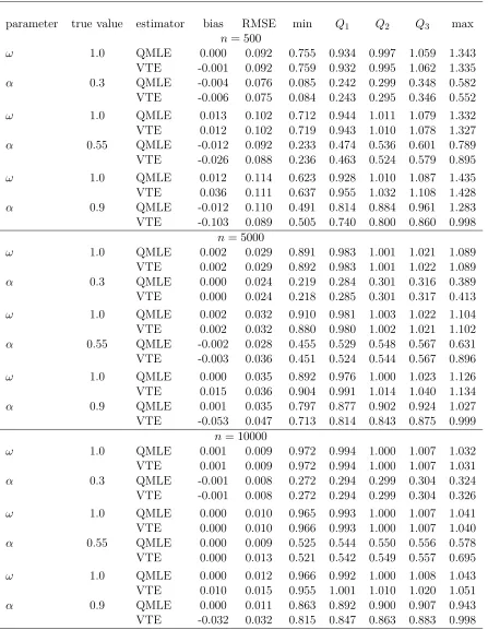
[image:9.612.64.523.173.262.2]

The most noticeable output is that the VTE performs remarkably well, and even outperforms the (Q)MLE when n = 500. This finite-sample result counterbalances the result of Proposition 3.1 showing that the VTE can not be asymptotically more efficient than the QMLE. As expected from Table 2, the QMLE and VTE ofω have very similar accuracy, and the QMLE ofα is slightly more accurate than the VTE whennis large (i.e. n= 5,000andn= 10,000) and α= 0.55orα= 0.9.

Table 1: Asymptotic variances of the QMLE and VTE of

ϑ

0

for an ARCH(1) with

γ

0

= 1

and

ηt

_{∼ N}

(0

,

1)

.

α

0

= 0

.

1

α

0

= 0

.

3

α

0

= 0

.

5

α

0

= 0

.

55

α

0

= 0

.

7

QMLE

2

.

52 0

.

51

0

.

51 1

.

69

4

.

80 2

.

24

2

.

24 2

.

84

12

.

01 5

.

71

5

.

71

3

.

93

15

.

94 7

.

11

7

.

11

4

.

20

45

.

27 14

.

32

14

.

32

5

.

02

VTE

2

.

52 0

.

51

0

.

51 1

.

69

5

.

06 2

.

36

2

.

36 2

.

90

18

.

13 8

.

61

8

.

61

5

.

30

28

.

78 12

.

82

12

.

82

6

.

74

[image:9.612.63.524.346.435.2]

∞

∞

means that the asymptotic variance does not exist

Table 2: Asymptotic variances of the QMLE and VTE of

θ

0

for an ARCH(1) with

ω

0

= 1

and

ηt

_{∼ N}

(0

,

1)

.

α

0

= 0

.

1

α

0

= 0

.

3

α

0

= 0

.

5

α

0

= 0

.

55

α

0

= 0

.

7

QMLE

3

.

5

−

1

.

4

−

1

.

4

1

.

7

4

.

2

−

1

.

8

−

1

.

8

2

.

8

4

.

9

−

2

.

2

−

2

.

2

3

.

9

5

.

1

−

2

.

2

−

2

.

2

4

.

2

5

.

6

−

2

.

4

−

2

.

4

5

.

1

VTE

3

.

5

₋

1

.

4

−

1

.

4

1

.

7

4

.

2

₋

1

.

8

−

1

.

8

2

.

9

4

.

9

₋

1

.

9

−

1

.

9

6

.

1

5

.

1

₋

2

.

1

−

2

.

1

9

.

3

∞

4.3

Comparison of the QMLE and VTE on daily stock market returns

In this section, we consider daily returns of 11 indices, namely the CAC, DAX, DJA, DJI, DJT, DJU, FTSE, Nasdaq,1 _{Nikkei, SMI and SP500. The samples extend from January 2, 1990, to January 22, 2009,} except for the indices for which such historical data do not exist. For each series, a GARCH(1,1) model was estimated, by QMLE and by VTE. Table 4 displays the models estimated by the two procedures. For these series of daily returns, it seems that the moment assumptionEǫ4

t <∞ is questionable, because

(ˆα+ ˆβ)2_{+ (Eη}d4

0 −1)ˆα2 is often close to or larger than 1, and it is known that Eǫ4t < ∞ if and only if

(α0+β0)2+ (Eη04−1)α20 <1. Therefore, the assumptions given in Theorem 3.1 to obtain the asymptotic

normality are likely to be unsatisfied. Nevertheless, it is seen from Table 4 that the parameters estimated by VTE are always very close to those estimated by QMLE.

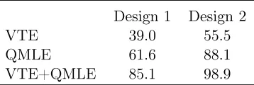
As expected, the VTE is more successful than the QMLE in terms of amount of computation time. Table 5 compares the computation time of the QMLE and VTE for estimating the models of the 11 indices. Two designs, corresponding to two different initial values, are considered. Design 1 corresponds to the initial valuesα= 0.05, β = 0.85and ω equal to (1₋α₋β) times the empirical variance of the series. Design 2 corresponds to the initial valuesα= 0, β= 0andω = 1. The initial values of Design 1 are much closer to

[image:10.612.71.518.73.650.2]

Table 3: Sampling distribution of the QMLE and VTE of

θ

0

for ARCH(1) models with

ηt

∼ N

(0

,

1)

.

parameter

true value

estimator

bias

RMSE

min

Q

1

Q

2

Q

3

max

n

= 500

ω

1.0

QMLE

0.000

0.092

0.755

0.934

0.997

1.059

1.343

VTE

-0.001

0.092

0.759

0.932

0.995

1.062

1.335

α

0.3

QMLE

-0.004

0.076

0.085

0.242

0.299

0.348

0.582

VTE

-0.006

0.075

0.084

0.243

0.295

0.346

0.552

ω

1.0

QMLE

0.013

0.102

0.712

0.944

1.011

1.079

1.332

VTE

0.012

0.102

0.719

0.943

1.010

1.078

1.327

α

0.55

QMLE

-0.012

0.092

0.233

0.474

0.536

0.601

0.789

VTE

-0.026

0.088

0.236

0.463

0.524

0.579

0.895

ω

1.0

QMLE

0.012

0.114

0.623

0.928

1.010

1.087

1.435

VTE

0.036

0.111

0.637

0.955

1.032

1.108

1.428

α

0.9

QMLE

-0.012

0.110

0.491

0.814

0.884

0.961

1.283

VTE

-0.103

0.089

0.505

0.740

0.800

0.860

0.998

n

= 5000

ω

1.0

QMLE

0.002

0.029

0.891

0.983

1.001

1.021

1.089

VTE

0.002

0.029

0.892

0.983

1.001

1.022

1.089

α

0.3

QMLE

0.000

0.024

0.219

0.284

0.301

0.316

0.389

VTE

0.000

0.024

0.218

0.285

0.301

0.317

0.413

ω

1.0

QMLE

0.002

0.032

0.910

0.981

1.003

1.022

1.104

VTE

0.002

0.032

0.880

0.980

1.002

1.021

1.102

α

0.55

QMLE

-0.002

0.028

0.455

0.529

0.548

0.567

0.631

VTE

-0.003

0.036

0.451

0.524

0.544

0.567

0.896

ω

1.0

QMLE

0.000

0.035

0.892

0.976

1.000

1.023

1.126

VTE

0.015

0.036

0.904

0.991

1.014

1.040

1.134

α

0.9

QMLE

0.001

0.035

0.797

0.877

0.902

0.924

1.027

VTE

-0.053

0.047

0.713

0.814

0.843

0.875

0.999

n

= 10000

ω

1.0

QMLE

0.001

0.009

0.972

0.994

1.000

1.007

1.032

VTE

0.001

0.009

0.972

0.994

1.000

1.007

1.031

α

0.3

QMLE

-0.001

0.008

0.272

0.294

0.299

0.304

0.324

VTE

-0.001

0.008

0.272

0.294

0.299

0.304

0.326

ω

1.0

QMLE

0.000

0.010

0.965

0.993

1.000

1.007

1.041

VTE

0.000

0.010

0.966

0.993

1.000

1.007

1.040

α

0.55

QMLE

0.000

0.009

0.525

0.544

0.550

0.556

0.578

VTE

0.000

0.013

0.521

0.542

0.549

0.557

0.695

ω

1.0

QMLE

0.000

0.012

0.966

0.992

1.000

1.008

1.043

VTE

0.010

0.015

0.955

1.001

1.010

1.020

1.051

α

0.9

QMLE

0.000

0.011

0.863

0.892

0.900

0.907

0.943

VTE

-0.032

0.032

0.815

0.847

0.863

0.883

0.998

[image:11.612.111.483.81.431.2]

Table 4: Comparison of the QMLE and VTE of GARCH(1,1) models for 11 daily stock market

returns. The estimated standard deviation are displayed into brackets. The last column corresponds

to plug-in estimates of

ρ

4

= (

α

+

β

)

2

+ (

Eη

04

−

1)

α

2

. We have

Eǫ

4

0

<

∞

if and only if

ρ

4

<

1

.

Index

estimator

ω

α

β

ρ

4

CAC

QMLE

0.033 (0.009)

0.090 (0.014)

0.893 (0.015)

1.0067

VTE

0.033 (0.009)

0.090 (0.014)

0.893 (0.015)

DAX

QMLE

0.037 (0.014)

0.093 (0.023)

0.888 (0.024)

1.0622

VTE

0.036 (0.013)

0.095 (0.022)

0.888 (0.024)

DJA

QMLE

0.019 (0.005)

0.088 (0.014)

0.894 (0.014)

0.9981

VTE

0.019 (0.005)

0.089 (0.012)

0.894 (0.007)

DJI

QMLE

0.017 (0.004)

0.085 (0.013)

0.901 (0.013)

1.002

VTE

0.016 (0.004)

0.085 (0.012)

0.901 (0.013)

DJT

QMLE

0.040 (0.013)

0.089 (0.016)

0.894 (0.018)

1.0183

VTE

0.042 (0.013)

0.086 (0.016)

0.894 (0.018)

DJU

QMLE

0.021 (0.005)

0.118 (0.016)

0.865 (0.014)

1.0152

VTE

0.021 (0.004)

0.119 (0.013)

0.865 (0.013)

FTSE

QMLE

0.013 (0.004)

0.091 (0.014)

0.899 (0.014)

1.0228

VTE

0.013 (0.004)

0.090 (0.013)

0.899 (0.014)

Nasdaq

QMLE

0.025 (0.006)

0.072 (0.009)

0.922 (0.009)

1.0021

VTE

0.025 (0.006)

0.072 (0.009)

0.922 (0.009)

Nikkei

QMLE

0.053 (0.012)

0.100 (0.013)

0.880 (0.014)

0.9985

VTE

0.054 (0.012)

0.098 (0.013)

0.880 (0.015)

SMI

QMLE

0.049 (0.014)

0.127 (0.028)

0.835 (0.029)

1.0672

VTE

0.048 (0.014)

0.133 (0.025)

0.834 (0.029)

SP500

QMLE

0.014 (0.004)

0.084 (0.012)

0.905 (0.012)

1.0072

VTE

0.014 (0.003)

0.084 (0.011)

0.905 (0.012)

the final estimates than those of Design 2. Thus, it is not surprising to observe longer computation times in Design 2 than in Design 1. In both designs, the QMLE is around 1.6 times slower than the VTE, and the time required for the 2 estimates (QMLE+VTE) is not much bigger than that taken by the QMLE. More interestingly, an examination of the estimated models shows that, in Design 2 (i.e. when the initial values are far from the final estimates) and for two indices (namely the DJI and SP500) the QMLE is trapped in a local estimate for which the likelihood is less than for the solution obtained in Design 1. For the VTE, and also for VTE+QMLE method, the solutions obtained in the two designs are the same. From these experiments, one can conclude that i) when the initial values are reasonably well chosen (in Design 1), there is no sensible differences between the estimated parameters of the two methods; ii) the VTE is a little bit faster and seems more robust relatively to the choice of the initial values; iii) the VTE provides good initial values for the QMLE and may avoid that this estimator be trapped in local optima.

4.4

Variance targeting estimator in misspecified models

[image:12.612.203.382.94.154.2]

Table 5:

Comparison of the computation time of the QMLE and VTE (in seconds of CPU time), for estimating the models of the 11 indices of Table 4. The method VTE+QMLE consists in using the VTE as initial values for the QMLE. Design 1 and 2 correspond to different initial values (see the text).

Design 1

Design 2

VTE

39.0

55.5

QMLE

61.6

88.1

VTE+QMLE

85.1

98.9

ergodic with a finite second order moment. This is generally not the case when the misspecified model is estimated by QMLE.

In the next sections, we consider two applications where this robustness feature of the VTE is particularly attractive.

4.4.1

Prediction over long horizons with models estimated by VTE

We will study the asymptotic behavior of the GARCH(1,1) predictions when the forecast horizon is large, and when the data generating process (DGP) may be different from the GARCH(1,1) model in (2.1). The results of this section can be extended to general GARCH(p, q)models, but the presentation will be simpler with GARCH(1,1) models. With the (possibly misspecified) GARCH(1,1) model, h-step ahead prediction intervals forǫn+h are given by

hq

ˆ σ2

n+h|nFˆ

−1 η (α/2),

q

ˆ σ2

n+h|nFˆ

−1

η (1−α/2)

i

,

where1−αis the nominal asymptotic probability of the interval,Fˆη(α)denotes an estimate of theα-quantile of the distributionFη ofη1, andσˆ_n+h2 _|n is the estimate of the h-step ahead forecast error variance, given by

ˆ

σ_n+h2 _|n = ˆγn∗+

n

σ2n(ˆϑ

∗

n)−γˆn∗

o_(1−κˆ∗

n)h+1

1−ˆκ∗

n when the GARCH model is estimated by QMLE, and by

ˆ

σ2n+h|n= ˆσn2+

n

σt2(ˆϑn)−σˆ2n

o_(1−ˆκn)h+1

1₋κˆn

when the GARCH model is estimated by VTE. When the GARCH(1,1) model is misspecified, the true parameter valueϑ0 does not exist, but one can expect that the QMLE and VTE converge to some so-called "pseudo" true values. More precisely, under stationarity, ergodicity and other general conditions, see White (1982),ϑˆ∗_n→ϑ˜∗ = (˜γ∗_,λ˜∗_{)almost surely asn→ ∞, where the pseudo true valueϑ˜}∗ _{is defined by}

˜

ϑ∗= arg min

ϑ Eℓ1(ϑ), ℓt(ϑ) =

ǫ2 t σ2

t(ϑ)

+ logσ2

t(ϑ).

Similarly, one should generally have

ˆ

ϑn →ϑ˜ = (˜γ,λ˜) a.s. withγ˜=Eǫ21andλ˜= arg min_λ Eℓ1(˜γ,λ).

Assume that these pseudo-true valuesλ˜ = (˜α,˜κ)andλ˜∗= (˜α∗_,˜κ∗_{)are such thatκ <˜ 1 andκ˜}∗_{<1. When}

the horizonhis large, the asymptotic prediction interval is thus equivalent to

hp

˜ γ∗_F−1

η (α/2),

p

˜ γ∗_F−1

η (1−α/2)

i

horizon h

Prediction interval

5 10 15 20

−10

−5

0

5

10

exact asymp QMLE VTE

horizon h

Prediction interval

5 10 15 20

−10

0

5

10

[image:13.612.92.479.24.179.2]

exact asymp QMLE VTE

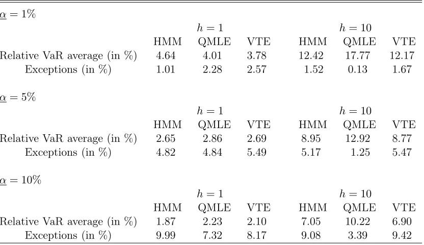
Figure 1:

Asymptotic prediction intervals based on the true model (between the full lines), for a GARCH(1,1) estimated by QMLE (dotted lines) and a GARCH(1,1) estimated by VTE (dashed lines). The horizontal full lines are the bounds of the large-horizon prediction intervals (4.1). The DGP is the Markov-switching model (4.3). The figure on the left corresponds to predictions when the present volatility σn is low, and the figure on the right corresponds to predictions in the case whenσn is large.

with the QMLE, and equivalent to

q

Eǫ2

1Fη−1(α/2),

q

Eǫ2

1Fη−1(1−α/2)

, (4.2)

with the VTE. Note that the long horizon prediction intervals (4.1) obtained with QMLE are not correct when˜γ∗

6

=Eǫ2

1, which is generally the case for misspecified models. On the contrary, even when the model is misspecified, the probability thatǫn+h belongs to the VTE asymptotic prediction interval (4.2) tends to the nominal probability1₋αas the horizonhincreases.

Example 4.1 To give an elementary illustration, consider the Markov-switching model

ǫt=ω(∆t)ηt, (4.3)

where ηt is an iid noise, (∆t)is a stationary irreducible and aperiodic Markov chain, independent of (ηt), with state-space_{1, . . . , d_}. For Figure 1, we tookηt∼ N(0,1),d= 2 regimes withω(1) = 1andω(2) = 5, and the transition probabilitiesP(∆t= 1_|∆t−1= 1) =P(∆t= 2|∆t−1= 2) = 0.9. It can be noted that(ǫt) is a white noise and that (ǫ2

t) is an autocorrelated process. Therefore, it is not unrealistic to assume that an empirical researcher would fit a misspecified GARCH model to data generated by Model (4.3). In our experiments, we fitted a GARCH(1,1) model by the two methods, on a simulation of size 1,000 of Model (4.3). Figure 1 shows the h-step ahead prediction intervals obtained from the true model and from the estimated GARCH models. It can be seen that, in particular when the prediction horizonh is large, the prediction intervals based on the false GARCH(1,1) model estimated by VTE are close to those obtained with the right model. When the GARCH parameters are estimated by QMLE, the prediction intervals are clearly oversized when the horizon h is large (indicating a pseud-true value γ˜∗ _{larger than Eǫ}2

1, for this particular model).

4.4.2

Estimating long horizon Value-at-Risk

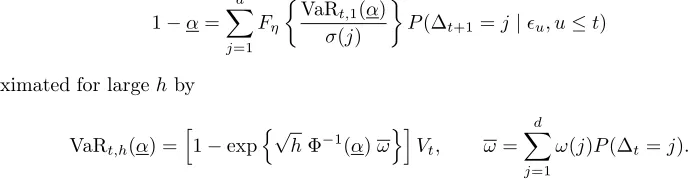
confidence levelα_∈(0,1), the horizonhand the datet, the (conditional) VaR is the(1₋α)-quantile of the conditional distribution ofLt,t+h given the information available at timet:

VaRt,h(α) = inf{x∈R_{|P(Lt,t+h≤x|Vu, u≤t)≥1−α}.}

Introducing the log-returnsǫt= log(Vt/Vt−1), we have

VaRt,h(α) = [1−exp{qt,h(α)}]Vt, (4.4)

where qt,h(α) is the α-quantile of the conditional distribution of the future returnsǫt+1+· · ·+ǫt+h. The following lemma shows how to approximate VaRt,h(α)for largeh, under some α-mixing condition on the process(ǫt).

Lemma 4.1 Assume that(ǫt)is a strictly stationary process such that Eǫt= 0,P∞h=1{αǫ(h)} ν/(2+ν)

<_∞ andE_|ǫt|2+ν <∞for someν >0. Let Var(ǫt) =ω2. We have

lim h→∞

√

h ωΦ−1(α)/qt,h(α) = 1 a.s.

Remark 4.1 The mixing condition of the lemma is satisfied for a variety of processes, in particular GARCH-type processes (see for instance Carrasco and Chen (2002) and Francq and Zakoïan (2006). This condition is also satisfied for the Markov-switching process (4.3). Indeed, the Markov chain(∆t)enjoys a number of mixing properties (seee.g. Theorem 3.1 in Bradley, 2005). In particular, there exist K >0 and ρ_∈(0,1) such that α∆(k) _≤ Kρk _{for all k}

∈ N_{. Because (ηt) and (∆t) are independent, and ǫt is a measurable}

function of∆tandηt, Theorem 5.2 in Bradley (2005) entails thatαǫ(k)≤Kρk_.

For any conditionally heteroscedatic process of the formǫt=σt(θ0)ηt, whereηt∼Fη, the VaR at horizon 1 is given by

VaRt,1(α) =1₋expσt(θ0)Fη−1(1−α) Vt,

in view of (4.4). Hence, ifθˆnis an estimator ofθ0, an obvious estimator of VaRt,1(α)is obtained by plugging. In general, exact VaR’s at horizonh >1cannot be computed explicitly. It is therefore of interest to use the previous lemma to approximate the VaR at a long horizonh. Given an estimatorωb ofω, one can take

d

VaRt,h(α) =h1₋expn√hΦ−1(α)ωboiVt. (4.5)

When (ǫt) follows a GARCH model, both the VTE and the QMLE methods provide consistent estima-tors of ω. When the GARCH model is misspecified, only the VTE guarantees consistency of ωb, and thus asymptotically valid estimates for long horizon VaR’s. This is illustrated in the next example.

Example 4.2 (Example 4.1 continued) We shall consider VaR at horizonsh= 1 andh= 10 obtained from estimated GARCH(1,1) models, when the observations are drawn from the Markov-switching process (4.3). For the sake of comparison, we shall also consider the theoretical VaR’s of the true model, obtained at horizon 1 as the solution of

1−α=

d

X

j=1 Fη

VaRt,1(α) σ(j)

P(∆t+1=j|ǫu, u≤t)

and approximated for largehby

VaRt,h(α) =h1₋expn√hΦ−1(α)ωoiVt, ω= d

X

j=1

[image:14.612.102.446.539.630.2]

ω(j)P(∆t=j).

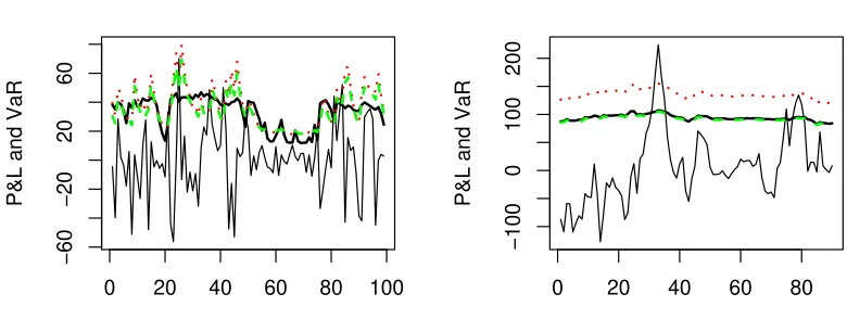
Figure 2 shows samples paths ofLt,t+h, forh= 1and h= 10, obtained with ηt∼ N(0,1), d= 2regimes,

ω(1) = 1/200andω(2) = 5/200. The full line indicates the VaR at the 5% level, computed with the true

his large. This is not the case for the VaR estimated by QMLE (dotted lines), which strongly overestimates

for h= 10. Standard evaluation of the performance of VaR estimation methods relies on comparing the

[image:15.612.88.504.225.465.2]

percentages of exceptions (losses larger than the estimated VaR) with the nominal levelα, on out-of-sample observations. Such a procedure is often referred to as "backtesting". Table 6 displays the average VaR (in percentages of the portfolio value Vt, that is 100/NPN_t=1VaRt,h(α)/Vt) together with the number of violations, over a very long period of time. This table confirms the conclusions drawn from Figure 2: the VaR at the horizonh= 10 computed with the misspecified GARCH(1,1) is more satisfactory in terms of backtesting when the model is estimated by VTE than by QMLE.

Table 6:

Backtesting comparison of the VaR estimations given by the true HMM model (4.3), the GARCH(1,1) model estimated by QMLE, and the GARCH(1,1) estimated by VTE on n = 1,000 obser-vations. The comparison is made out-of-sample, on a simulation of sizeN = 50,000of the profit and loss (P&L) function, for the two horizonsh= 1andh= 10and the three levelsα= 1%,α= 5%andα= 10%.

α

= 1%

h

= 1

h

= 10

HMM

QMLE

VTE

HMM

QMLE

VTE

Relative VaR average (in %)

4.64

4.01

3.78

12.42

17.77

12.17

Exceptions (in %)

1.01

2.28

2.57

1.52

0.13

1.67

α

= 5%

h

= 1

h

= 10

HMM

QMLE

VTE

HMM

QMLE

VTE

Relative VaR average (in %)

2.65

2.86

2.69

8.95

12.92

8.77

Exceptions (in %)

4.82

4.84

5.49

5.17

1.25

5.47

α

= 10%

h

= 1

h

= 10

HMM

QMLE

VTE

HMM

QMLE

VTE

Relative VaR average (in %)

1.87

2.23

2.10

7.05

10.22

6.90

Exceptions (in %)

9.99

7.32

8.17

9.08

3.39

9.42

5

Conclusion

VTE is a two-step estimation method which reduces the computational complexity of the optimization procedure and guarantees that the implied variance is equal to the sample variance. This paper provides asymptotic results for the VTE, allowing for valid inference procedures, such as tests or the construction of confidence intervals, based on this method. This paper also compares the asymptotic and empirical performances of the VTE to the standard QMLE.

One evident drawback of the VTE is that the existence ofE(ǫ4

VaR at horizon h=1

P&L and VaR

0 20 40 60 80 100

−60

−20

20

60

VaR at horizon h=10

P&L and VaR

0 20 40 60 80

−100

0

100

[image:16.612.90.480.12.159.2]

200

Figure 2:

Sample paths of the P&L process generated by the Markov-switching model (4.3) and VaR at the confidence level 5%. The full line corresponds to the exact VaR, the doted (resp. dashed) line to the asymptotic approximation obtained from Lemma 4.1 applied to a GARCH model estimated by QMLE (resp. VTE).

be smaller than that of the QMLE; ii) the variance targeting may result in a serious deterioration of the asymptotic precision when the moment condition is close to be violated. On the other hand, the finite sample performance of the VTE seems quite satisfactory. Moreover, our experiments on daily stock returns do not show sensible differences between the estimated parameters of the two methods. Finally, we have shown that, for some specific purposes such as long-term prediction, the fact that the VTE guarantees a consistent estimation of the long-run variance may be a crucial advantage of the VTE over the QMLE.

While this paper has provided evidence there is value in considering a VTE in GARCH models, there remain interesting questions in this area. Other moments could be targeted, not only the long run variance, and it would be interesting to examine the asymptotic properties of the resulting estimators. In particular, in a multivariate framework, "correlation targeting" has been considered by Engle (2002) for the specification of the dynamic conditional correlation model.

Appendix: proofs

Let

ln(λ) =n−1 n

X

t=1

ℓt(γ0,λ), ℓt(γ,λ) =ℓt(ϑ) = ǫ2

t σ2

t(ϑ)

+ logσt2(ϑ).

Fort_≥1we define

˜

ℓt(ϑ) = ǫ 2 t ˜ σ2

t(ϑ)

+ log ˜σt2(ϑ).

In this appendix, the lettersK andρdenote generic constants, whose values can vary along the text, but always satisfyK >0and0< ρ <1.

A.1

Proof of consistency in Theorem 2.1

We will follow the proof that Francq and Zakoïan (2004), hereafter FZ, gave for the strong consistency of the QMLE θˆ∗_n. This result also entails the consistency of ϑˆ∗_n, but is not directly applicable to show the consistency of ϑˆn, because the VTE is a two-step estimator which is not expressible as a function of the QMLE.

The almost sure convergence of σˆ2

suffices to establish the following results.

i) lim

n→∞λsup∈Λ|l

n(λ)₋˜ln(λ)_|= 0, a.s.

ii) if σt2(γ0,λ) =σt2(γ0,λ0) a.s., then λ=λ0, iii) if λ₆=λ0, then Eℓt(γ0,λ)> Eℓt(γ0,λ0),

iv) any λ₆=λ0has a neighborhoodV(λ)such that lim inf

n→∞ λ∗_∈inf_V(λ)

˜_ln(λ∗

)> Eℓ1(γ0,λ0) a.s.

We first showi). Note that the difference between ln(λ)and˜ln(λ) is due to the replacement ofγ0 by ˆσn2, and is also due to the initial values taken forǫ0andσ20(γ0,λ). To handle simultaneously the two sources of difference, note that

σ2t,n(λ)−σt2(γ0,λ) =κ(ˆσn2−γ0) +β

σt2−1,n(λ)−σt2−1(γ0,λ)

=κ(ˆσ2

n−γ0)

1₋βt

1−β +β

t_σ2

0−σ02(γ0,λ) .

Thus, sinceσˆ2

n converges toγ0 almost surely, we have sup

λ_∈Λ|

σ2t,n−σ2t(γ0,λ)| ≤Kρt+o(1) a.s.

Note thatK is a measurable function of_{ǫu, u≤0}.For the almost sure consistency, the trajectory is fixed in a set a probability one andntends to infinity. ThusK can be considered as a constant,i.e. Kis almost surely invariant withn. The point i)follows from

sup

λ_∈Λ|l

n(λ)₋˜ln(λ)_{| ≤}n−1 n

X

t=1 sup

λ_∈Λ

(

σ2

t,n−σt2(γ0,λ) σ2

t,nσt2(γ0,λ)

ǫ

2 t+

log 1 +

σ2

t(γ0,λ)−σt,n2 σ2

t,n

! )

≤

sup

λ_∈Λ

1 κ2

₁

γ0ˆσ2 n

Kn−1 n

X

t=1 ρtǫ2t+

sup

λ_∈Λ

1 κ

₁

ˆ σ2

n Kn−1

n

X

t=1

ρt+o(1)

and the arguments used in the proof in FZ.

The requirementsii)andiii)have already been proven in FZ in a more general framework (see the proof of their Theorem 2.1). The proof ofiv) is also a direct adaptation of the proof given in FZ. For the reader convenience, we briefly restate the proofs ofii)-iv) in our particular GARCH(1,1) framework. To showii) note that

σt2(ϑ) = κγ

1₋β +α

∞

X

i=0

βiǫ2t−i−1. (A.1)

Suppose thatσ2

t(ϑ) =σ2t(ϑ0)a.s.Then, in view of (A.1), κγ

α+κ+α

∞

X

i=0

βiǫ2t−i−1= κ0γ0 α0+κ0

+α0

∞

X

i=0

β0iǫ2t−i−1.

Because the innovation ofǫ2

t is nota.s.equal to zero underA2, we must have κγ

α+κ = κ0γ0 α0+κ0

, and αβi=α0β0i ∀i≥0.

This entailsϑ=ϑ0.

To showiii), we argue that forx >0,logx_≤x₋1,with equality if and only ifx= 1. We thus have

Eℓt(ϑ)₋Eℓt(ϑ0) =Elog σ 2 t(ϑ) σ2

t(ϑ0)

+Eσ

2 t(ϑ0) σ2

t(ϑ) − 1

≥E

log σ

2 t(ϑ) σ2

t(ϑ0)

+ logσ

2 t(ϑ0) σ2

t(ϑ)

with equality if and only ifσ2

t(ϑ0)/σt2(ϑ) = 1a.s., which is equivalent toϑ=ϑ0in view ofii).

Let us show iv). Let Vk(λ) be the open ball with centerλ and radius 1/k. Using successively i), the ergodic process, the monotone convergence theorem andiii), we obtain almost surely

lim inf

n→∞ λ∗_∈Vinf_k(λ_)∩Λ

˜_ln(λ∗₎

≥lim inf

n→∞ λ∗_∈Vinf_k(λ_)∩Λln(λ

∗₎

−lim sup

n→∞ λsup_∈Λ|l

n(λ)₋˜ln(λ)_|

≥lim inf

n→∞ n −1

n

X

t=1 inf

λ∗_∈Vk(λ)∩Λℓt(γ0,λ

∗₎

=E inf

λ∗_∈Vk(λ_)∩Λℓ1(γ0,λ

∗₎

> Eℓ1(γ0,λ0)

forklarge enough, whenλ₆=λ0.

A.2

Proof of asymptotic normality in Theorem 2.1

The proof of the asymptotic normality rests classically on a Taylor-series expansion of each component of the score vector aroundϑ0. In comparison to the proof given by FZ for the QMLE, additional difficulties come from the fact that the VTE is a two-step estimator. On the other hand, the proof of of some technical parts will be facilitated by the assumptionEǫ4

t <∞. Although restrictive, this moment assumption is required for the asymptotic normality of the empirical varianceσˆ2

n. Writeλ= (λ1, λ2)and ϑ= (ϑ1, ϑ2, ϑ3). Noting that, in (2.10),ℓt,n(λ) = ˜ℓt(ˆσ2

n,λ), we have

(0,0)′=n−1/2

n

X

t=1 ∂

∂λℓt,n(ˆλn) =n

−1/2 n

X

t=1 ∂ ∂λℓ˜t(ˆϑn)

=n−1/2

n

X

t=1 ∂

∂λℓ˜t(ϑ0) +

1 n n X t=1 ∂2 ∂λi∂ϑj

˜ ℓt(ϑ∗_i)

!

2×3 √

nϑˆn−ϑ0

=n−1/2

n

X

t=1 ∂

∂λℓ˜t(ϑ0) +Jn

√

nλˆn−λ0

+Kn√n σˆn2−γ0 (A.2)

where theϑ∗i are betweenϑˆn andϑ0,

Jn= 1 n

n

X

t=1 ∂2 ∂λi∂λj

˜ ℓt(ϑ∗_i)

!

2×2

, Kn= 1 n n X t=1 ∂2 ∂γ∂λ1 ˜ ℓt(ϑ∗₁),1

n n X t=1 ∂2 ∂γ∂λ2 ˜ ℓt(ϑ∗₂)

!′

.

We will show that

i)E

∂ℓt(_∂ϑϑ0)

∂ℓt(ϑ0) ∂ϑ′

<∞, E ∂

2_ℓt(ϑ0) ∂ϑ∂ϑ′

<∞,

ii)A:=E

1 σ4

t(ϑ0) ∂σ2

t(ϑ0) ∂ϑ

∂σ2 t(ϑ0) ∂ϑ′

is non-singular and Var

∂ℓt(ϑ0) ∂ϑ

=Eη40−1 A,

iii) there exists a neighborhoodV(ϑ0)ofϑ0 such that, for alli, j, k∈ {1, . . . , p+q+ 1},

E sup

ϑ_∈V(ϑ0) ∂

3_ℓt(ϑ) ∂ϑi∂ϑj∂ϑk

<∞,

iv) n −1/2 n X t=1 (

∂ℓt(ϑ0) ∂ϑ −

∂ℓ˜t(ϑ0) ∂ϑ

)

→0 and ϑ∈Vsup(ϑ0) n −1 n X t=1 (

∂2_ℓt(ϑ) ∂ϑ∂ϑ′ −

∂2_ℓ˜t(ϑ) ∂ϑ∂ϑ′

) →0

in probability whenn_{→ ∞},

v)n−1 n

X

t=1 ∂2 ∂ϑi∂ϑj

ℓt(ϑ∗k)→A(i, j)a.s.

vi)Xn:=

n1/2 σˆ2n−γ0 n−1/2Pn

t=1 ∂ ∂λℓt(ϑ0)

⇒ N

0,(Eη40−1)

b 0

0 J

The derivatives ofℓt=ǫ2t/σt2+ logσ2t are given by

∂ℓt(ϑ) ∂ϑ =

1₋ ǫ

2 t σ2 t 1 σ2 t ∂σ2 t ∂ϑ

(ϑ), (A.3)

∂2_ℓt(ϑ) ∂ϑ∂ϑ′ =

1− ǫ

2 t σ2 t 1 σ2 t ∂2_σ2

t ∂ϑ∂ϑ′

(ϑ) +

2ǫ 2 t σ2 t − 1 1 σ2 t ∂σ2 t ∂ϑ 1 σ2 t ∂σ2 t ∂ϑ′

(ϑ). (A.4)

The same formulas hold for the derivatives ofℓ˜t, with σ2

t replaced byσ˜t2. Forϑ=ϑ0,ǫ2

t/σ2t =η2t is independent of the terms involvingσ2t and its derivatives. To provei)it will therefore be sufficient to show that

E

σ12

t ∂σ2

t ∂ϑ(ϑ0)

<∞, E σ12

t ∂2_σ2

t ∂ϑ∂ϑ′(ϑ0)

<∞, E σ14

t ∂σ2 t ∂ϑ ∂σ2 t ∂ϑ′(ϑ0)

<∞. (A.5)

The following expansions hold

∂σ2 t ∂ϑ(ϑ) =

κ

1−β,

−κγ

(1−β)2+

∞

X

ℓ=0

βℓǫ2t−ℓ−1−α

∞

X

ℓ=1

ℓβℓ−1ǫ2t−ℓ−1, αγ

(1−β)2 −α

∞

X

ℓ=1

ℓβℓ−1ǫ2t−ℓ−1

!′

.

Recall thatA3impliesEǫ4t <∞. Moreover we haveσt−2(ϑ0)≤κ−01γ0−1 <∞. This allows us to prove the first and third inequalities in (A.5). The second inequality is proved by exactly the same arguments, andi) is proved. Note that we made use of the moment assumptionEǫ4

t <∞to facilitate the proof of (A.5). This moment assumption is actually unnecessary. Indeed, we will show, without this assumption, that for any integerd, there exists a neighborhood_V(ϑ0)ofϑ0 such that

E sup θ∈V(ϑ0)

_σ12

t ∂σ2 t ∂ϑi d

<_∞, E sup θ∈V(ϑ0)

_σ12

t ∂2_σ2

t ∂ϑi∂ϑj

d

<_∞ E sup θ∈V(ϑ0)

_σ12

t

∂3_σ2 t ∂ϑi∂ϑj∂ϑk

d

<_∞. (A.6)

Choose_V(ϑ0)small enough, so that all the parametersγ, κ, α andβ be bounded away from zero. Using the elementary inequalityx/(1 +x)_≤xs _{for allx}

≥0and alls_∈(0,1], for allϑ_{∈ V}(ϑ0)we have

σ12

t ∂σ2t

∂γ (ϑ)

≤K, _σ12

t ∂σ2

t ∂α (ϑ)

≤K+

∞

X

ℓ=0

βℓ_ǫ2 t−ℓ−1 K+αβℓ_ǫ2

t−ℓ−1

+α

∞

X

ℓ=1

ℓβℓ−1_ǫ2 t−ℓ−1 K+αβℓ_ǫ2

t−ℓ−1

≤K+K

∞

X

ℓ=0

βℓsǫ2st−ℓ−1+K

∞

X

ℓ=0

ℓβℓsǫ2st−ℓ−1.

Similarly

σ12

t ∂σ2

t ∂κ (ϑ)

≤K+K

∞

X

ℓ=0

βℓsǫ2st−ℓ−1+K

∞

X

ℓ=0

ℓβℓsǫ2st−ℓ−1.

Under 2.5 we haveEǫ2

t <∞andsupϑ_∈V(ϑ0)β <1. Thuskǫ

2s

t kd<∞for somes∈(0,1], and the first result of (A.6) comes from the Hölder inequality. The other results of (A.6) are obtained with the same arguments. Now we proveii). IfAis singular, there existsx= (x1, x2, x3)6= 0such thatx′∂σ2t(ϑ0)/∂ϑ = 0a.s. Since

∂σ2 t ∂ϑ =

∂κγ ∂ϑ +

∂α ∂ϑǫ

2 t−1+

∂β ∂ϑσ

2 t−1+β

∂σ2 t−1

∂ϑ , (A.7)

the strict stationarity ofσ2

t(ϑ0)implies

x′∂κγ

∂ϑ (ϑ0) +x

′∂α

∂ϑ(ϑ0)ǫ

2 t−1+x′

∂β ∂ϑσ

2

We thus have

x1κ0+x3γ0+x2ǫ2t−1= (x2+x3)σt2−1(ϑ0) a.s.

This entails thatx2ǫ2t−1is a function of{ǫ2t−i, i >1},which is impossible underA2, unlessx2= 0.We then obtain thatx3 = 0because σt2−1(ϑ0)is not almost surely constant. It then follows thatx1= 0. Finally we obtained a contradiction and the non-singularity ofAis proved.

Let us proveiii). Differentiating (A.4), we obtain

∂3_ℓt(ϑ) ∂ϑi∂ϑj∂ϑk

=

1₋ ǫ

2 t σ2 t 1 σ2 t

∂3_σ2 t ∂ϑi∂ϑj∂ϑk

(ϑ) +

2ǫ 2 t σ2 t − 1 1 σ2 t ∂σ2 t ∂ϑi 1 σ2 t ∂2_σ2

t ∂ϑj∂ϑk

(ϑ) (A.8)

+ 2ǫ 2 t σ2 t − 1 1 σ2 t ∂σ2 t ∂ϑj 1 σ2 t ∂2_σ2

t ∂ϑi∂ϑk

(ϑ) +

2ǫ 2 t σ2 t − 1 1 σ2 t ∂σ2 t ∂ϑk 1 σ2 t ∂2_σ2

t ∂ϑi∂ϑj

(ϑ)

+

2−6ǫ

2 t σ2 t 1 σ2 t ∂σ2 t ∂ϑi 1 σ2 t ∂σ2 t ∂ϑj 1 σ2 t ∂σ2 t ∂ϑk

(ϑ).

Becauseinfϑ∈V(ϑ0)σ

2

t(ϑ)>0 andEǫ4t<∞, we have

E sup

ϑ_∈V(ϑ0)

1₋ ǫ

2 t σ2

t(ϑ)

2

<_∞, E sup

ϑ_∈V(ϑ0) 2ǫ 2 t σ2 t − 1 2

<_∞, E sup

ϑ_∈V(ϑ0)

2₋6ǫ

2 t σ2 t

2 <_∞.

In view of this result and of (A.6) withd= 1,2,3, the Hölder inequality entailsiii). We now turn to the proof ofiv). In view of (2.8) and (2.11), we have

σ2t(ϑ)−σ˜2t(ϑ) =βt

σ02(ϑ)−˜σ02 .

Therefore, choosing_V(ϑ0)such thatλ_∈Λfor allϑ_{∈ V}(ϑ0), we have

sup

ϑ∈V(ϑ0)

σt2(ϑ)−σ˜t2(ϑ)

_≤Kρt, sup

ϑ∈V(ϑ0) ∂σ

2 t(ϑ) ∂ϑ −

∂˜σ2 t(ϑ) ∂ϑ

≤Kρt

and

sup

ϑ_∈V(ϑ0) σ21

t(ϑ)− 1 ˜ σ2

t(ϑ)

=ϑ_∈Vsup₍ϑ0) σ21

t(ϑ)

˜

σ2t(ϑ)−σ2t(ϑ) 1 ˜ σ2

t(ϑ)

≤Kρt.

In view of (A.3), we then obtain

sup

ϑ∈V(ϑ0) n −1 n X t=1 (

∂ℓt(ϑ) ∂ϑ −

∂ℓ˜t(ϑ) ∂ϑ ) ≤Kn −1 n X t=1

ρtΥt, a.s., (A.9)

where

Υt= sup

ϑ_∈V(ϑ0)

1 + ǫ

2 t σ2 t

1 + 1

σ2 t ∂σ2 t ∂ϑ

(ϑ).

UsingEǫ4

t <∞,infϑ_∈V(ϑ0)σ

2

t(ϑ)>0 and (A.6), the Cauchy-Schwarz inequality shows thatEΥt<∞. By the Borel-Cantelli lemma, it follows thatρt_{Υt→0a.s.and thus the right-hand side of (A.9) converges to 0} a.s.Using the same arguments, and replacing first derivatives with second derivatives,iv) is shown.

Similarly to the proof of (4.36) in FZ,v)follows from the Taylor expansion ofn−1Pn

t=1∂2ℓt(ϑ

∗

k)/∂ϑi∂ϑj aroundθ0, the convergence of ϑ∗k to θ0, and iii).

The proof ofvi)relies on a Central Limit Theorem for martingale differences. From Horváth, Kokoszka and Zitikis (2006, Proof of Theorem 1) (see (A.15) below) we have the representation

ˆ

σ2n=γ0+

1₋β0

κ0 1 n n X t=1

ht(η2t−1) +oP(n−1/2). (A.10)

Moreover, in view of (A.3)

n−1/2 n

X

t=1 ∂

∂λℓt(ϑ0) =n

−1/2 n

X

t=1

1−η2

t ht

∂σ2 t

We then have

Xn =n−1/2 n

X

t=1

(1₋ηt2)Zt+oP(1), Zt=

−(1₋β0)κ−01ht h−t1∂σ2t(ϑ0)/∂λ

. (A.12)

Notice that E (1₋η2

t)Zt|Ft−1 = 0, where Ft is the σ-algebra generated by the random variables ǫt−i,

i_≥0. Moreover, we have

∂σ2 t ∂α =ǫ

2

t−1−σ2t−1+β ∂σ2

t−1 ∂α =

∞

X

i=0

βi(ǫ2t−i−1−σ2t−i−1),

∂σ2 t

∂κ =γ−σ 2 t−1+β

∂σ2 t−1 ∂κ =

∞

X

i=0

βi(γ₋σ2t−i−1),

and thus

E

_∂σ2 t ∂λ(ϑ0)

= 0. (A.13)

It follows that

Var(1−η2t)Zt = (Eη04−1)

b 0

0 J

.

Notice thatbis a positive real number and that the matrix J in the right-lower block ofAis non-singular, in view of the non-singularity of A. By assumptionsA2andA3, we get 0< Eη4

0−1<∞, and thus the matrix Var(1−η2

t)Zt is nondegenerate. Hence for any λ ∈ R3, the sequence (1−η2t)λ

′

Zt,Ft _t is a square integrable stationary martingale difference. By (A.12), the central limit theorem of Billingsley (1961) and the Wold-Cramer device we obtain the asymptotic normality ofXn, which proves v).

To complete the proof of the theorem, note that, from ii), iv) and v), it follows that the matrix Jn is a.s.invertible for sufficiently largen. Therefore, in view of (A.2),

√

nλˆn−λ0

=−J−_n1

(

n−1/2 n

X

t=1 ∂

∂λℓ˜t(ϑ0) +Kn

√

n σˆ2n−γ0

)

.

It follows that, usingiv),

√ n

_σˆ2 n−γ0 ˆ

λn−λ0

=

_{1 0}

−J−n1Kn −J−n1

Xn+oP(1).

Thus, byv), vi)and Slutsky’s lemma, √nϑˆn−ϑ0

is asymptoticallyN(0,Σ)distributed, with

Σ=

1 0

−J−1K ₋J−1

b 0

0 J

1 ₋K′J−1

0 ₋J−1

.

The invertibility ofΣ follows and the proof of Theorem 2.1 is complete.

A.3

Proof of Corollary 2.1

This corollary of Theorem 2.1 can be proven by a direct application of the delta method (seee.g. Theorem 3.1 in van der Vaart, 1998). Indeed the mapφwhich transformsϑ0 intoθ0 is differentiable atϑ0, and the Jacobian matrix of this map is

∂φ

∂ϑ′0 =



 ∂(∂αγ0κ00)/∂γ/∂γ0 0 ∂(∂αγ0κ0/∂α0)/∂α0 0 ∂(∂αγ0κ00)/∂κ/∂κ0 0 ∂(1₋κ0−α0)/∂γ0 ∂(1−κ0−α0)/∂α0 ∂(1−κ0−α0)/∂κ0

A.4

Proof of Corollary 2.2

It is known that for an invertible partitioned matrix

A=

A11 A12

A21 A22

,

ifA11 is invertible, then we have

A−1=



 F −F A12A

−1 22

−A−221A21F A−221+A−221A21F A12A−221

 ,

whereF = (A11−A12A22−1A21)−1. Using this classical result we get

Σ∗=

a ₋aK′J−1

−aJ−1K J−1+aJ−1KK′J−1

, a=

_κ2 0

(α0+κ0)2E

₁

h2 t

−K′J−1K −1

,

whereas

Σ=

b −bK′J−1

−bJ−1K J−1+bJ−1KK′J−1

, b=(α0+κ0) 2

κ2 0

E(h2t).

Thus

Σ−Σ∗= (b₋a)

1 ₋K′J−1

−J−1K J−1KK′J−1

,

and the result follows.

A.5

Proof of Theorem 3.1

The consistency can be obtained as in FZ, by a direct extension of Theorem 2.1. Let us concentrate on the asymptotic normality. Similarly to (A.2), we have

0p+q=n−1/2

n

X

t=1 ∂ ∂λℓ˜t(ˆϑn)

=n−1/2

n

X

t=1 ∂

∂λℓ˜t(ϑ0) +

1 n

n

X

t=1 ∂2 ∂λi∂ϑj

˜ ℓt(ϑ∗i)

!

(p+q)×(p+q+1) √

nϑˆn−ϑ0

=n−1/2

n

X

t=1 ∂

∂λℓ˜t(ϑ0) +Jn

√

nλˆn−λ0

+Kn√n σˆn2−γ0, (A.14)

where theϑ∗_i are betweenϑˆn andϑ0,

Jn= 1 n

n

X

t=1 ∂2 ∂λi∂λj

˜ ℓt(ϑ∗_i)

!

(p+q)×(p+q) ,

Kn= 1 n

n

X

t=1 ∂2 ∂γ∂λ1

˜

ℓt(ϑ∗1), . . . , 1 n

n

X

t=1 ∂2 ∂γ∂λp+q

˜ ℓt(ϑ∗p+q)

!′

.

We now use the ARMA representation forǫ2 t:

ǫ2t =ω0+ p∨q

X

i=1

(α0i+β0i)ǫ2t−i+νt−

p

X

j=1

β0jνt−j,

withνt= ǫ2t−ht =ht(η2t −1) and obvious conventions. Taking the average of both sides of the equality whentvaries from 1 ton, we obtain

ˆ

σ2n=ω0+ p∨q

X

i=1

(α0i+β0i)ˆσ2n+

 1−

p

X

j=1 β0j

 1

n n

X

t=1