A New Aware Context Collaborative Filtering Approach by Applying Multivariate Logistic Regression Model into General User Pattern

http://dx.doi.org/10.4236/jdaip.2016.43011

A New Aware-Context Collaborative

Filtering Approach by Applying

Multivariate Logistic

Regression Model into

General User Pattern

Loc Nguyen

Sunflower Soft Company, Ho Chi Minh City, Vietnam

Received 12 September 2016; accepted 15 August 2016; published 18 August 2016

Copyright © 2016 by author and Scientific Research Publishing Inc.

This work is licensed under the Creative Commons Attribution International License (CC BY).

http://creativecommons.org/licenses/by/4.0/

Abstract

Traditional collaborative filtering (CF) does not take into account contextual factors such as time, place, companion, environment, etc. which are useful information around users or relevant to re-commender application. So, recent aware-context CF takes advantages of such information in or-der to improve the quality of recommendation. There are three main aware-context approaches: contextual pre-filtering, contextual post-filtering and contextual modeling. Each approach has in-dividual strong points and drawbacks but there is a requirement of steady and fast inference model which supports the aware-context recommendation process. This paper proposes a new approach which discovers multivariate logistic regression model by mining both traditional rating data and contextual data. Logistic model is optimal inference model in response to the binary question “whether or not a user prefers a list of recommendations with regard to contextual con-dition”. Consequently, such regression model is used as a filter to remove irrelevant items from recommendations. The final list is the best recommendations to be given to users under contex-tual information. Moreover the searching items space of logistic model is reduced to smaller set of items so-called general user pattern (GUP). GUP supports logistic model to be faster in real-time response.

Keywords

1. Introduction

Recent researches on collaborative filtering (CF) focus on inherent information about users and items and how to recommend such relevant items to such users. Database used to build up CF algorithms is in form of rating matrix composed of ratings that users give to items. Additional contextual factors such as time, place, condition and situation existing in real world are not considered in CF algorithms. For instance, if a user prefers to watch news program in morning and movies in evening then contextual information, namely temporary information, should be aware in recommendation tasks and so, it is inappropriate to provide movies to her/him in the morning even though such movies are the most relevant to her/him.

Given a training set which is a rating matrix and a user who requires recommendations, CF algorithm tries to predict rating value on items which are not rated by this user. After that CF algorithm makes a list of such items arranged in order of predictive rating values and recommends this user such list. In other words, CF algorithm constructs a predictive function R2 ([1], pp. 217-250) whose cross domain is the Cartesian product of a set of users U and a set of items I. The domain U × I is also called rating matrix. Co-domain of function R2 is a set of predictive ratings denoted R.

2U I :

R × U× →I R

Function R2 called traditional 2-dimension (2D) mapping doesn’t consider contextual factors now and it can lack information necessary to highly accurate prediction. Suppose contextual information including location, time and companion are added to prediction process, the 2D function R2 becomes the 3-dimension (3D) map-ping denoted as below:

3U I C:

R × × U× × →I C R

Note that C, U × I and U × I × C represent context domain, 2D (cross) domain and 3D (cross) domain, respec-tively. In order words, function R3 gives recommendations to user under circumstances specified as contextual information.

Although context has many different types, we can reduce these types into three main types in order to answer three question forms: when, where and who ([1], pp. 224-225).

 Time type indicates the time when user requires recommendation, for example: date, day of week, month, and year.

 Location type indicates the place where user requires recommendation, for example: theater, coffee house.

 Companion type indicates the persons with whom user goes or stays when recommendation task is required, such as: alone, friends, girlfriend/boyfriend, family, co-workers.

Contextual information is organized in two forms: hierarchical structure ([2], p. 1537) and multi-dimensional data (MD) model.

According to hierarchical form, the context domain C is defined as a set of contextual dimension K = (K1, K2,

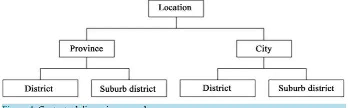
K3, ∙∙∙, Kn). K is represented in hierarchy structure, whose attributes Ki(s) are associated with the ascending order of fine level. For example, given attributes Ki and Kj where I < j, Kj is finer than Ki and so Ki contains Kj. It is easy to recognize that K1 is the coarsest attribute which contains all remaining attributes K2, K3∙∙∙, Kn. Each Ki

contains values at the same level i and it can be split into finer levels. An example of contextual dimension is shown in Figure 1.

In above example, K2 = {City, Province}, K3= (City → District, City → Suburb district, Province → District,

[image:2.595.140.488.605.713.2]

Province → Suburb district).

According to MD form, context domain C is defined as the Cartesian product of n dimension, C = D1 × D2 ×

∙∙∙× Dn. Each dimension Di, in turn, is a set of attributes, Di = (ai1, ai2, ∙∙∙, aik). For example, suppose C has only

one dimension of time denoted D1 = Time (day of week). So, the cross domain U × I × C of predictive function

[image:3.595.218.419.570.709.2]

R3 constitutes a 3D cube: User (name), Item (book name) and Time (day of week). Each block in this cube is as-signed a rating which is the predictive outcome of function R3. Figure 2 depicts a MD cube ([1], p. 227).

Figure 2 indicates that given user “John” (101), item “novel book” (7) and time “Sunday” (1), the predictive outcome of R3 gains the highest value 5.

There are three approaches ([1], pp. 232-233) to apply context into recommendation process:

 Contextual pre-filtering: Firstly, given context c∈C is used to select user-item pairs (u, i) which are more relevant to this context, leading to obtain the aware-context cross domain U × I. After that traditional 2D function R2 is taken on such cross domain.

 Contextual post-filtering: Firstly, traditional 2D function R2 is used to produce the list of recommended item. After that context C is used to fine-tune this list in order to remove irrelevant items according to concrete context.

 Contextual modeling: The 3D function R3 is used directly on context-aware cross domain U × I × C.

The basic idea of contextual pre-filtering is to project the 3D domain U × I × C on 2D plane, based a concrete context c∈C so that such 3D domain is reduced to 2D domain U × I. Let ∏c be projection operation based

on condition context c, we have:

(

)

c

U I C U I ∏ × × = ×

(

)

( )

( )

3 , , 2 ,

c

U I C U I C

R _{× ×} u i c =R _{∏ × ×} u i

The concrete context c∈C which is strict projection condition can make the cross domain U × I small or sparse, causing low predictive accuracy. So generalization technique is used to make projection condition loose, namely the exact condition c is replaced by the more general condition c’. For example, the context c = “Satur-day” which indicates that “Mary prefers to go shopping on Satur“Satur-day” is replaced by more flexible context c = “Weekend” because she can like going shopping on Sunday if she often goes on Saturday. The general context not only expends the space of potential recommendation solutions but also improve predictive accuracy.

The essence of contextual post-filtering is to fine-tune the raw recommendation results taken from predictive function R2 which didn’t consider contextual factors before. Consequently, this method tries to figure out user’s context-aware interests, preferences or attributes by using some artificial intelligent and mining techniques and apply such attributes into raw results so as to remove out irrelevant items or change their ranks in final recom-mendation list. For example, given context c = “evening” which indicates Mary’s interest “watching movies in the evening”, contextual post-filtering approach will remove all of news or sport events from her recommenda-tion list.

The strong point of contextual pre-filtering and post-filtering approaches is the ability to take advantage of legacy recommendation algorithms not taking account into contextual factors.

The essence of contextual modeling is to incorporate directly contextual information into predictive function

R3 and so, R3 is constructed as inference model such as data mining, machine learning, heuristic model or sta-tistical model, etc. The 2D predictive function isn’t used in contextual modeling. It implies that the strong

point of this method is pure and powerful inference mechanism. It opens a new trend in context-aware recom-mendation research, giving a lot of prospects although a few related techniques are extensions of 2D algorithms. The approach in this paper is the hybrid of contextual post-filtering and contextual modeling. Hence a logistic inference model ([3], pp. 372-411) is used as the post filter to make recommendations more relevant to users according to contextual factors. Section 2, which is the main section, describes the proposed approach in detail. The concept of general user pattern (GUP) is firstly introduced and then the collaborative filtering algorithm based on GUP and logistic model is mentioned. The equation to solve logistic model, which is the most impor-tant feature of the proposed algorithm, is constructed with support of mathematical tools. An example is given at the end of section 2 for illustrating the proposed approach. Section 3 is the conclusion.

2. Basic Idea and Details of the New Approach

The new approach is suggested by two comments:

 Although contextual information is necessary to improve the quality of recommendation process but it can-not replace essential rating information in collaborative filtering research. Inference model taking into ac-count contextual factor should be used as the filter to adjust recommendations returned from predictive rat-ings so as to give users more appropriate items in concrete circumstances.

 When additional contextual information is considered, the speed of recommendation process is decreased. So inference mechanism should be fast in real-time response.

The basic idea is to apply a fast inference model, namely logistic regression function into a list of recom-mended items so as to achieve a better recommendation result under contextual information. The logistic regres-sion model responses immediately the binary request “whether or not a list of items is relevant to concrete con-text or preferred by users”. Because there are various items and each item is associated with an individual re-gression function, the domain of rere-gression function becomes huge, which decreases the speed of algorithm. In order to solve this problem, the items space is reduced to “general user pattern”.

General user pattern (GUP) is known as a set of items to which “many” users give ratings. Since rating values on GUP are not always high, it reflects solely user’s access or rating frequency. Given the threshold θ, let n and

nj be the number of total users and the number of users who rate on item xj, we have:

{

j j

}

where j

GUP= x n n x I

So GUP is defined as a set of items where the ratio of the number of total users to the number of users who rate on such each item is great than or equal to a given threshold θ.

Given a GUP, context c and a logistic regression function f, the regressive (or independent) variables of f are taken from GUP. The response of f is binary variable taking values between 0 and 1 where value 1 indicates that it is likely that user prefers GUP under context c and otherwise. Suppose GUP = {x1, x2, ∙∙∙, xn}, logistic

regres-sion function f (x1, x2, ∙∙∙, xn) can be considered to be dependent on GUP.

Given the raw recommended list R, an instance of GUP is initialized on R. This instance denoted INS is a set of predictive rating values taken from R with condition that respective items co-exist in both R and GUP. For example, if R = {x1 = 5, x2 = 3, x3 = 4} and GUP = {x1, x3} then INS = {x1 = 5, x3 = 4} because item x1 and

item x3 exist in both R and GUP and their respective values are 5 and 4.

Consequently, regression model f is evaluated on INS with regard to context c∈C. If the outcome of f with

INS is near to 0 then all items in GUP are removed from R. Finally, the list R is recommended to user after it was fine-tuned by pruning irrelevant items from it.

In general the algorithm has four steps:

1) A 2D predictive function is applied into rating matrix U × I so as to produce a raw list R of recommended items without existence of contextual factors.

2) GUP is discovered over contextual 3D cross domain U × I × C. Items in GUP are frequent items. 3) Multivariate logistic function f is learned from cross domain U × I × C by statistical technique.

4) Function f is used to remove irrelevant items from the list R. In other words, only aware-context items are kept in R. So the final filtered list is the best result which is recommended to users. This step includes two sub- steps:

a) The instance of GUP so-called INS is constructed by matching GUP with R.

Because step 3 is the most important, the method to construct multivariate logistic function is discussed in detailed now. The probability that GUP = {x1, x2, ∙∙∙, xn} belongs to context c∈C is p; in other words, the

probability that user prefers GUP under context c is p. The concept odd ([3], p. 11.8) is defined as the ratio of p

to 1 − p. This ratio represents how much user likes GUP vice versa how much user dislikes item GUP.

1

p odd

p =

−

Note that the odd also expresses how likely GUP belongs to context c∈C vice versa how likely GUP does not belongs to context c. The natural logarithm of odd is linear regression function of n variables being GUP.

(

)

0 1 1 2 2

log log log log

1 n n

p

odd x x x

p α α α α

 

= _{ }= + + + +

−

   (1)

Note that x1, x2, ∙∙∙,and xn are regressive or independent variables whose values are obtained from

recom-mended list R later and coefficients αi(s) are called parameters of logistic model. If odd is considered as response

or dependent variable, Equation (1) is re-written as following:

(

0 1 1 2 2

)

exp

1 n n

p

odd x i x x

p α α α

= = + + + +

−  (2)

where exp(∙) denotes exponent function.

The probability p that user likes items in GUP is computed according to following function derived from Eq-uation (2) with attention that such probability is logistic regression function f (x1, x2, ∙∙∙, xn).

(

)

(

)

(

)

1 2

0 1 1 2 2

1 , , ,

1 exp

n

n n

f i i i p

x x x

α α α α

= =

+ − + + + +



 (3)

Equation (3) represents the multivariate logistic model f with regard to a concrete context c. The approach in this paper uses this equation to estimate whether or not a user prefers a list of recommended items based on a concrete context. For example, given user being “John”, GUP being {“Gladiator”, “Golden Eye”}, recom-mended movie list being {“Gladiator” with predictive rating 5, “Golden Eye” with predictive rating 4, “Four Rooms” with predictive rating 4} and, if f produces a value greater than or equal to 0.5 when f is evaluated on

GUP with regard to time context “evening”, then it asserts that John likes such list and there is no film to be re-moved. This logistic model is built up in offline mode so as not to affect response time.

The problem needs solved now is to determine parameters αi(s) in logistic function f. We will use method of

maximum likelihood estimate (MLE) [4] to construct them. Given training data D is rating cube whose dimen-sions are user, item and context. Each volume in rating cube is quantified by a value that a user rate on an item in concrete context. If rating cube is projected onto a context c, we get a rating matrix Dc with two dimensions

such as user and item. Suppose Dc has m rows and n columns and let yi= (yi1, yi2, ∙∙∙, yin) be the ith row of Dc and

it is easy to infer that yij is the ith instance (rating value) of item xj. Suppose rating values yij(s) range from 1 to v

where v-most favorite and 1-most dislike and the value 0 indicates that user does not rate on item. Suppose GUP

also has n items which are the same to ones in Dc, let ai= (ai1, ai2, ∙∙∙, ain) be a possible instance of such n items.

Hence, there are (v+1)n such instances because aij ranges from 0 to v. For example, if n = 2 and v = 2 we have 9

instances (0, 0), (0, 1), (0, 2), (1, 0), (1, 1), (1, 2), (2, 0), (2, 1), (2, 2). Let zi be the number of yi in Dc so that yi = ai and so there are N = (v+1)n such zi(s). Let pi be an instance of logistic function f evaluated on x1 = yi1, x2 = yi2,

∙∙∙, xn = yin, we have:

(

)

(

0 1 1 2 2

)

1 1 exp

i

i i n in

p

y y y

α α α α

=

+ − + + + +

It is easy to infer that pi is the probability that the instance ai occurs in Dc. The likelihood function ([4], p. 4)

of f given training data Dc is:

(

0 1 2

)

(

)

(

)

1 1

, , , , 1 1

1

i i

zi

N N

N z N

z i

n i i i

i i i

p

L p p p

p

α α α α −

= =

 

= − = _{ } −

−

 

∏

∏

 (4)

(

0 1 2

)

(

)

1

0 0

1 1 1

, , , , log 1 1

log 1 exp

i z N N i n i i i

N n n

i j ij j ij

i j j

p

LogL p

p

z y N y

α α α α

α α α α

= = = =  _{ }    = _{ } −  _ − _          = _  + − _ +  + __       

∏

∑

∑

∑

 (5)

The first order partial derivatives of logarithm likelihood function with regard to αk(s) are:

(

)

(

)

(

)

(

)

1 1 1 0 1 0 ₀ 0 0 1 1 exp 1 exp exp where 1 1 exp

N _{j ij}

i _n

i

j ij n

N _{j ij}

n j j j i j

ik i _n

k _{j ij}

N y LogL z y N y LogL

y z k n

y

α α

α _{α α}

α α

α _{α α}

= = = = = =  ₊  ∂ _{=  − }   ∂ _{ + + }    ₊  ∂ _{=  −  ≤ ≤}   ∂ _{ + + }           

∑

∑

∑

∑

∑

∑

If there is convention that yi0 = 1, we have:

(

)

(

00

)

1 1 1 exp where 0 1 exp n

N _{j ij}

ik i _n

k _{j i}

j i

j j

N y

LogL

y z k n

y

α α

α _{α α}

= = =  ₊  ∂ _{=  −  ≤ ≤}   ∂ _{ + + }  

∑

∑

∑

(6)

Let α α0*, 1*,, and αn* be estimates of α0, α1, ∙∙∙, and αn, respectively. These

( )

*

k s

α are maximum points of logarithm likelihood function and hence, we set the first order partial derivatives of logarithm likelihood func-tion with regard to αk

( )

s so as to find out

( )

* k s α .

(

)

(

)

(

)

(

)

(

)

(

)

0 0 0 0 0 1 0 1 1 1 1 1 1 1 1 1 1 1 1 1 1 0 0 0 exp ₁ 1 exp 0 exp ₁ 0 1 exp 0 _exp 1 1 exp n N

N _{i j ij}

i i n

j ij n

N _{i j ij} N

i i n

j ij

n

N _{in j ij} N

n in j i i i n j j i i j j i

j j ij i

y y

y z

LogL _y N

y y LogL y z N y LogL y y y z N y α α α α α α α

α _{α α}

α α α α α = = ₌ = = = = = = = = = + = ∂ _{= + +} ∂ + ∂ = = ∂ _{+ +} ∂ = ₊ ∂ = +  ⇔  +

∑

∑

∑

∑

∑

∑

∑

∑

∑

∑

∑

∑

                                (7)

Because Equation (7) is the set of n + 1 non-linear equations with n + 1 variables, it is easy to find out its solu-tion (α α0*, 1*,,αn*) by applying some numerical analysis methods such as Newton-Raphson ([5], pp. 67-79)

me-thod. Substituting estimates α α*0, 1*,,α*n into Equation (3), it is totally to determine the logistic function f.

For example, suppose there are 2 items, GUP= {x1, x2} receiving binary values such as 0-dislike and 1-like.

So, we have n = 2, v = 1 and 4 possible instances y1 = (y11 = 0, y12 = 0), y2 = (y21 = 0, y22 = 1), y3 = (y31 = 1, y32 = 0),

y4 = (y41 = 1, y42 = 1). According to Equation (2), instances of logistic function f evaluated on y1, y2, y3, and y4 are:

(

)

(

)

₍

₎

(

)

(

)

₍

₎

(

)

(

)

₍

₎

(

)

(

)

₍

₎

1 11 12 1 2

0

2 21 22 1 2

0 2

3 31 32 1 2

0 1

4 41 42 1 2

0 1 2

1

0, 0 0, 0

1 exp

1

0, 1 0, 1

1 exp

1

1, 0 1, 0

1 exp

1

1, 1 1, 1

1 exp

p f y y f x x

p f y y f x x

p f y y f x x

p f y y f x x

α

α α

α α

α α α

Suppose only instance y1 = (y11 = 0, y12 = 0) is observed and so we have z1 = 1, z2 = z3 = z4 = 0. The Equation

(7) becomes:

( )

( )

(

(

)

)

(

(

)

)

(

(

)

)

(

)

(

)

(

(

)

)

(

)

(

)

(

(

)

)

0 0 1 0 2 0 1 2

0 0 1 0 2 0 1 2

0 1 0 1 2

0 1 0 1 2

0 2 0 1 2

0 2 0 1 2

4 exp 4 exp 4 exp 4 exp

1 0

1 exp 1 exp 1 exp 1 exp

4 exp 4 exp

0

1 exp 1 exp

4 exp 4 exp

0

1 exp 1 exp

α α α α α α α α

α α α α α α α α

α α α α α

α α α α α

α α α α α

α α α α α

+ + + +

− − − − =

+ + + + + + + +

+ + +

− − =

+ + + + +

+ + +

−   

− =

+ + + + +

     

It is necessary to solve Equation (7) with regard to coefficients α0, α1, and α2. Suppose α0 = 0 and α2 = α1, we

have:

( )

( )

( )

( )

( )

( )

( )

( )

1 1

1 1

1 1

1 1

8 exp 4 exp 2

1 0

1 exp 1 exp 2

4 exp 4 exp 2 0 1 exp 1 exp 2

α α

α α

α α

α α

− − =

+ +

−    

− =

+ +

  

By using software Mathematica [6], it is easy to find out α α0*, 1* and * 2

α as follows:

* 0

* *

1 2 2.15109 3.141

0

59i α

α α

 =

 

= = − +



where i= −1 is imaginary unit.

Finally, probabilities p1, p2, and p3 are determined by substituting complex solutions

* * 0, 1

α α and α*2 into

Equation (2) as follows:

(

)

(

)

(

)

(

)

1 1 2

17

2 1 2

17

3 1 2

18

4 1 2

0, 0 0.5

0, 1 0.131679 1.82495*10

0, 1 0.131679 1.82495*10

0, 1 0.0133582 3.2281*10 p f x x

p f x x i

p f x x i

p f x x i

−

−

−

= = = =

= = = = − + = = = = − +

= = = = −

where i= −1 is imaginary unit.

If GUP gets the instance y11 = (x1 = 0, x2 = 0), the logistic probability p1 = f (x1 = 0, x2 = 0) = 0.5 which leads

to conclude that user does not like such two items.

3. Conclusions

The approach in this paper is the hybrid of contextual post-filtering and contextual modeling where logistic model is applied in the post stage of recommendation process. The thinking behind this approach is that rating values obtained explicitly by questionnaires or implicitly by inferring users’ behaviors are the most important and contextual factor around users or related to application is additional information which is useful but not es-sential. Comparing to contextual pre-filtering, this approach restricts the loss of rating information in rating ma-trix by ignoring data pre-filtering. At the post stage, this approach removes only items which are asserted that users do not like them under contextual condition. Such assertion is the outcome of steady inference model, namely logistic model.

Acknowledgements

I express my deep gratitude to Prof. Dr. Ho, Hang T. T., Vinh Long General Hospital, Vietnam Ministry of Health who funded me to complete and publish this research.

References

[1] Ricci, F., Rokach, L., Shapira, B. and Kantor, P.B. (2011) Recommender Systems Handbook (Vol. I). Ricci, F., Ro-kach, L., Shapira, B. and Kantor, P.B., Eds., Springer, New York, Dordrecht, Heidelberg, London.

http://dx.doi.org/10.1007/978-0-387-85820-3

[2] Palmisano, C., Tuzhilin, A. and Gorgoglione, M. (2008) Using Context to Improve Predictive Modeling of Customers in Personalization Applications. IEEE Transactions on Knowledge and Data Engineering, 20, 1535-1549.

http://dx.doi.org/10.1109/TKDE.2008.110

[3] Montgomery, D.C. and Runger, G.C. (2003) Applied Statistics and Probability for Engineers. 3rd Edition, John Wiley & Sons, Inc., New York.

[4] Czepiel, S.A. (2002) Maximum Likelihood Estimation of Logistic Regression Models: Theory and Implementation.

http://czep.net

[5] Burden, R.L. and Faires, D.J. (2011) Numerical Analysis. Julet, M., Ed., 9th Edition, Brooks/Cole Cengage Learning, 872.

[6] Wolfram. (n.d.) Mathematica. Wolfram Mathematica, 10. http://www.wolfram.com/mathematica

Submit or recommend next manuscript to SCIRP and we will provide best service for you:

Accepting pre-submission inquiries through Email, Facebook, LinkedIn, Twitter, etc. A wide selection of journals (inclusive of 9 subjects, more than 200 journals) Providing 24-hour high-quality service

User-friendly online submission system Fair and swift peer-review system

Efficient typesetting and proofreading procedure

Display of the result of downloads and visits, as well as the number of cited articles Maximum dissemination of your research work