Inference Based on Empirical Likelihood for Varying Coefficient Model with Random Effect

http://dx.doi.org/10.4236/ojs.2013.36A006

Inference Based on Empirical Likelihood for Varying

Coefficient Model with Random Effect

Wanbin Li1,2, Liugen Xue1

1_{College of Applied Sciences, Beijing University of Technology, Beijing, China} 2_{Department of Mathematics, Yancheng Teachers University, Yancheng, China}

Email: [email protected], [email protected]

Received November 14, 2013; revised December 14, 2013; accepted December 21,2013

Copyright © 2013 Wanbin Li, Liugen Xue. This is an open access article distributed under the Creative Commons Attribution Li- cense, which permits unrestricted use, distribution, and reproduction in any medium, provided the original work is properly cited. In accordance of the Creative Commons Attribution License all Copyrights © 2013 are reserved for SCIRP and the owner of the intel- lectual property Wanbin Li, Liugen Xue. All Copyright © 2013 are guarded by law and by SCIRP as a guardian.

ABSTRACT

In this article, we develop a statistical inference technique for the unknown coefficient functions in the varying coeffi- cient model with random effect. A residual-adjusted block empirical likelihood (RABEL) method is suggested to inves- tigate the model by taking the within-subject correlation into account. Due to the residual adjustment, the proposed RABEL is asymptotically chi-squared distribution. We illustrate the large sample performance of the proposed method via Monte Carlo simulations and a real data application.

Keywords: Varying Coefficient Model; Random Effect; Empirical Likelihood; Longitudinal Data

1. Introduction

Varying coefficient model has been widely used to mod- el all kinds of data. One popular application is the analy- sis of the longitudinal data (e.g. [1,2]). Although both [3] and [4] proposed effective inference procedure for the varying coefficient model and applied them to the analy- sis of CD4 count data, whose detailed information can be referred to [5], none of them considered the within-sub- ject correlation of longitudinal data. To improve the effi- ciency of the inference by considering this kind of corre- lation, we consider the varying coefficient model with random effect

 

T T _,

ij ij ij ij i ij

Y X  T Z  e

m

(1) with i1, , , n j1, , , where 

 

 is an unknown smoothing p1 function vector, i are independent

vectors of random effect with mean 0 and covari- ance matrix D and ij are independent mean 0 random

variables with variance . Let ij and ij

1

l

e

2

e

 0 Y X , Zij, ij denote the response and covariate variable, respect-

tively, where the i and j are their associated jth measure-

ment of the ith subject among all of the longitudinal data. T

Random effect model is frequently employed to ex- ploit the characteristics of longitudinal data over several time periods. Recently, there has been fruitful research

on it. (e.g. [6-9]) proposed an efficient estimation for the single index model with random effect and provided a further way to construct the confidence interval for the parameter of interest with the aid of an estimator for its asymptotic variance.

correlation of longitudinal data. Also the estimation pro- cedure introduced in Section 2 makes the implementation much easier.

The rest of this article is organized as follows. In Sec- tion 2, we introduce the residual-adjusted block empirical likelihood method and provide details on constructing the confidence interval for the varying coefficient function of interest. Some asymptotic results are derived in Section 3 and several implementation issues are shown in Section 4. Simulations are reported in Section 5. Data arising from CD4 study is analyzed in Section 6. Proofs of the main results are relegated to Appendix.

2. Estimation Method

2.1. Empirical Likelihood Estimation

Assume that the observed data are gen- erated from model (1). Moreover, let ,

, i i1 im and

. Based on the idea of GEE [15], we can construct an auxiliary random vector nonparametric com- ponent





Y X Tij, ij, ij

1

i i

Y  Y





T

, , Z









t







T

, ,Yim





T

1, ,

i i im

X  X  X





T

1, ,

i i im

e  e  e

Z  Z

 





T 1



 

i t X Wi i i Yi Xi t

  _{ } _  ₍₂₎ where is the within-subject covariance matrix. De-

note i , where













1

diag , ,

i h i h im

W  K t t  K t

 

 

h

K  K

 





E t

h





 _i



0

with and being a kernel function and proper bandwidth, respectively. Note that if is the true parameter. There- fore, we can introduce an estimating equation as

 

K 

 

t

h 

 





1 0 n i i t    



, and a naive empirical log-likelihood ratio function for 

 

t can be derived as

 





 

 





1 1 1

2 max log 0, 1,

0 .

n n

i i i

i i

n i i i

l t np p p

p t                 







(3)

However, by the similar argument in [3], the proposed empirical log-likelihood ratio (3) is no longer a standard chi-square distribution unless an undersmoothing band- width is chosen. And some complicated techniques, such as Monte Carlo approximation or estimated transforma- tion, have to be employed to make further inference. For its limit being chi-square in practice, we propose a RABEL method by taking the ideal of [14] and [16]. Under the framework of RABEL, the auxiliary random vector function is newly defined as

 





T 1

 



   

i t X Wi i i Yi Xi t Xi ti t

  _{ } _{ }  _  _ _

   





(4)

where the estimator is a preliminary estimator. And the RABEL ratio is further derived as

 

t 

 





 

 





1 1 1

2 max log 0, 1,

0 .

n n

i i i

i i

n i i i

l t np p p

p t          _      







 _ (5)

By the Lagrange multiplier method, we have

 





T

1 1

, 1, , 1

i

i

p i

n    t



   n, (6) where  is a p1 vector satisfying

 





 





T 1

1 _{0, 1, , .}

1 n i i i t i n t         



   n m (7)

Then, the empirical likelihood ratio function (5) can be represented as

 







T



 





1

2n log 1 1 i , 1, , .

i

l  t    t i n







  

 _{  (8)}

2.2. Estimation of the Variance Component

The within-subject covariance i is assumed to be

known in the proposed RABEL procedure in Section 2.1. However, in practice, we need to construct an estimator for it. Assume that the model (1) satisfies the variance covariance-variance model



2_{1 1}T 2 _,

i  m m eI

   (9) where 1m represents an m1 vector of ones and I_m is the m m identity matrix. This proposed model (9) is

called a variance component model and widely used in longitudinal analysis, see, for example (e.g. [8,9]). Let

im , with ij



_



T

 ₁

i i, ,

   _ie_ij



2_,



. Hence, an estima- tor for the variance component 2



e

  is derived as





1 2

1 1 2 2

1 1

1 _{ˆ ˆ}

ˆ ,

1

n m

ij ij

i j j j

nm m        

 

 and 1 1 2 2 1 1 1 _ˆ

ˆe n m ij ,

i j nm 2      





 (10)

where with the preliminary estimator 

 

t for 

 

t ,

the residual ˆij is defined as

 

T

ˆij Yij Xij tij , i 1, , ,n j 1, , .m

     _  _

Therefore, we obtain the estimator for i, that is

2 T 2

ˆ _{ˆ 1 1 ˆ ,}

i  m m eIm

   (11) Furthermore, with the true covariance in (4) being in- terpolated by the estimator (11), we derive a new auxil- iary random vector

 





T 1

 



   



ˆ ˆ

i t X Wi i i Yi Xi t Xi ti t

  _{ } _{ }  _  _ _

   



And, the newly estimated RABEL ratio function is

 





 

 





1 1

1

ˆ _{2 max log 0, 1,}

ˆ _{0 .}

n n

i i i

i i

n i i i

l t np p p

p t



 

 





  _  



   











(13)

Additional implementation details of solving the pre- liminary estimator will be postponed to Section 4, after discussion of the asymptotic properties of the proposed method.

3. Asymptotic Result

In this section, we study the asymptotic properties of the estimators. Denote f

 

 to be the density for covariate

variable ij.

Theorem 1. Suppose that conditions (C1)-(C6) in the Appendix hold, then

T



_ˆ2 2



L



_{0, ,}

n __ N V_



(14)

and



_ˆ2 2



L



_0,



_,

e e e

n   N V (15)

where

 





2 2 4

2 1

4 2

1

e e

V Var

m m m

 

  



  

 and

 

4

2 11

2 . 1

e e

V Var e

m



 



Theorem 2. Suppose that conditions (C1)-(C7) in the Appendix hold. If is the true value of the parame- ter, then

 

t



 





2

ˆ L _,

p l  t 

 ₍₁₆₎

where 2p means a

2

 distribution with freedom p.

Note that p



2 ₁



  is the



1



quantile of 2

p

 . Based on Theorem 2, we can derive the



1



confi- dence interval of 

 

t , that is

 







 

ˆ



 



2



₁





_.

p

C_  t   t l  t  

4. Implementation Issue

4.1. Calculation of the Preliminary Estimator For t in the small neighborhood of 0, a Taylor expan- sion for the kth component of the varying coefficient

function leads to

t

 

t 

 



0



, 1, ,

k t ak b tk t k p

      , (17)

where

 

0

.

k k

t t

t b

t 



 



By ignoring the within-subject correlation, we can ob-

tain the unknown vector a, b by minimizing









2



T

0 0

1 1

,

n m

ij ij ij h ij

i j

Y X a b t t K t t

 

 _{  }  _

 





(18)

where a



a, , ap



T T

1 , 1 . Then, the so- lution to the minimization of (18) is



, , p

b b  b



   







0 0 0



0 0

T 1

T T T T

0 ˆ 0

ˆ , t t t t t ,

a t b t  D W D  D W Y

and









0

11

11 11 0 0

.

nm t

nm nm

X X

D

X t t X t t

 

  _{ } 

 

 

Specially, by the idea of local linear estimation, the preliminary estimator 

 

t0 is followed by

 







_{T0 0 0}



1 _{T0 0} 0 p,0p t t t t t .

t I D W D D W

   Y (19)

4.2. Choice of Bandwidth

As is well-known, the choice of bandwidth h can affect

both the bias and variance estimation and there is a trade- off between a proper bias and variance. A smaller vari- ance arise with the choice of a large bandwidth value, whereas will increase the estimation bias. As pointed out by [3,13], an optimal bandwidth, which is selected by using the leave-one-subject-out cross validation, can sat- isfy the conditions. Therefore, in the following simula- tions in this article, we use kernel function

 

_{0.75 1}



2



K u u



  and the optimal bandwidth is ob- tained by minimizing

 

 

 

2

T 1 1

, ,

n m

i

ij ij ij

i j

CV h Y X   t h

 

 





_   _

where  i

 

,

ij

t h

_ _{is denoted to be the preliminary es-}

timator (19) estimated with all over the measurements except the ith subject.

5. Empirical Study

In this section, we perform some Monte Carlo simula- tions to assess the finite sample performance of the pro- posed method. Assume the data is generated from the model

 

T _{, 1, , ; 1, , ,}

ij ij ij i ij

Y X  T  e i  n j  m (20)

where 

 

t 



₁

   

t ,₂ t



T with ₁

 

t sin



πt 2



and ₂

 

t  1 cos

 

πt . Moreover, we also assume that

 

0, 4 , 1, 2

ijk

X N 2 k and T_ij are generated from an

uniform distribution on interval [0,1]. Meanwhile, denote that



_0, 2



i N 

   and



_0, 2

ij e



e N  , where



 _, _e





procedure in this article, we apply it to the analysis of a longitudinal AIDS data set, reported by [5]. Some infer- ence methods are related in literatures of [3,4,17]. How- ever, there is limited work of them that focused on the within-subject correlation under the random effect frame- work. In fact, when we use the Hausman test for the null hypothesis of the random effect, the random effect is approved at 5% level of significance with p-value 85.9%,

which can be calculated by the R function phtest() in the plm package.

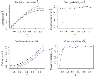
comparison, in addition to the proposed procedure during the simulations, a “naive” approach, based on the work- ing independence assumption, is also involved, assuming that the within cluster covariance matrices are identities. The simulation results were calculated by 100 runs.

Figure 1 reports the approximate 95% point-wise con- fidence intervals and their coverage probability curves for the coefficient function and , calcu- lated by the proposed method in this article and the “na- ive” method. Although from Figure 1, two methods con- struct close confidence intervals for the nonparametric component, the coverage probability curves in the right panels show a significant difference. The coverage prob- ability curves, estimated with the proposed method in this article, are closer to the significance lever 95% and possess a more stable and superior performance.

 

1 t

 ₂

 

t

As to the jth measurement of the ith subject, let ij be

CD4 percentage, ij be the time in years after HIV in-

fection, i1

Y t

Z be the centered age at HIV infection, Z_i2

be the centered preCD4 percentage, and Zi3 be the smoking status, taking a value of 1 or 0 for smoker or nonsmoker. Hence, we consider the following varying coefficient model with random effect

By the two required methods, we construct the simul- taneous confidence regions of at time point in Figure 2. The two plot are designed with



   



1 t ,2 t

1

t



e



 , being (0.1,0.1) and (0.2,0.1), respectively. Di- rect comparison of them illustrates the inference im- provement of the proposed RABEL method on that “na- ive” one.

 

 



 

0 ,1 1 ,2 2

,3 3 ,

ij ij ij ij ij ij

ij ij i ij

Y t Z t Z t

Z t e

  

 

  

  



(21)

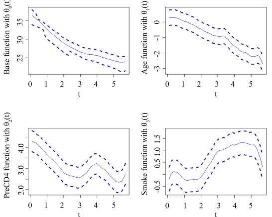
where the baseline CD4 percentage curve 0

 

t is used

to represent the mean CD4 percentage of t years after the

infection. By the proposed inference procedure in this article, we plot the curves of the unknown coefficient functions in model (21) and their approximate 95% con- fidence intervals in Figure 3. From the curve of baseline

6. Real Application

[image:4.595.137.457.423.683.2]

To illustrate the effectiveness of the proposed inference

[image:5.595.154.438.89.338.2]

Figure 2. The simultaneous confidence region of the two varying coefficient functions at point t = 1, with dashed and dotted- dashed curve being estimated by ignoring and considering the within-subject correlation, respectively. The left and right panel are for



 , e

 

 0.1, 0.1 and





 , e

 

 0.2, 0.1 , respectively.



Figure 3. The four plots show the changing curve and their corresponding 95% confidence interval for the different covariate variables as baseline curve, Age, PreCD4, and Smoke status.

function in Figure 3, we can find that the estimated curve of the mean CD4 percentage depletion over time also indicate that after getting infected, the CD4 counts decreases sharply at the first 4 years and then the de- creasing rate becomes slower although it sometimes changes a little, which is similar to the arguments in [3,

[image:5.595.163.436.399.617.2]

7. Acknowledgements

This work was partially supported by National Natural Science Foundation of China (11171012, Key program: 11331011), Science and Technology Project for the Su- pervisor of Excellent Doctoral Dissertation of Beijing (20111000503), Specialized Research Fund for the Doc- toral Program of Higher Education of China

(20121103110004) and the Beijing Municipal Key Dis- ciplines (No.006000541212010).

REFERENCES

[1] C. T. Chiang, J. A. Rice and C. O. Wu, “Smoothing Spline Estimation for Varying Coefficient Models with Repeatedly Measured Dependent Variables,” Journal of the American Statistical Association, Vol. 96, No. 454, 2001, pp. 605-619.

[2] A. Qu and R. Li, “Quadratic Inference Functions for Varying Coefficient Models with Longitudinal Data,” Biometrics, Vol. 62, No. 2, 2006, pp. 379-391.

http://dx.doi.org/10.1111/j.1541-0420.2005.00490.x [3] L. G. Xue and L. X. Zhu, “Empirical Likelihood for a

Varying Coefficient Model with Longitudinal Data,” Journal of the American Statistical Association,Vol. 102, No. 478, 2007, pp. 642-652.

http://dx.doi.org/10.1198/016214507000000293

[4] H. J. Wang, Z. Zhu and J. Zhou, “Quantile Regression in Partially Linear Varying Coefficient Models,” Annals of Statistics, Vol. 37, No. 6B, 2009, pp. 3841-3866. [5] R. A. Kaslow, D. G. Ostrow, R. Detels, J. P. Phair, B. F.

Polk and C. R. Rinaldo, “The Multicenter AIDS Cohort Study: Rationale, Organization and Selected Characteris- tics of the Participants,” American Journal of Epidemiol- ogy, Vol. 126, No. 2, 1987, pp. 310-318.

http://dx.doi.org/10.1093/aje/126.2.310

[6] Q. Li and A. Ullah, “Estimating Partially Linear Panel Data Models with One-way Error Components,” Econo- metric Reviews, Vol. 17, No. 2, 1998, pp. 145-166. http://dx.doi.org/10.1080/07474939808800409

[7] C. Gu and P. Ma, “Optimal Smoothing in Nonparametric Mixed Effect Models,” Annals of Statistics, Vol. 33, No. 3, 2005, pp. 1357-1379.

http://dx.doi.org/10.1214/009053605000000110

[8] J. You, X. Zhou and Y. Zhou, “Statistical Inference for Panel Data Semiparametric Partially Linear Regression Models with Heteroscedastic Errors,” Journal of Multi- variate Analysis, Vol. 101, No. 5, 2010, pp. 1079-1101. http://dx.doi.org/10.1016/j.jmva.2010.01.003

[9] Z. Pang and L. G. Xue, “Estimation for the Single-index Models with Random Effects,” Computational Statistics & Data Analysis, Vol. 56, No. 6, 2012, pp. 1837-1853. http://dx.doi.org/10.1016/j.csda.2011.11.007

[10] A. B. Owen, “Empirical Likelihood Ratio Confidence Intervals for a Single Functional,” Biometrika, Vol. 75, No. 2, 1988, pp. 237-249.

http://dx.doi.org/10.1093/biomet/75.2.237

[11] A. Owen, “Empirical Likelihood Ratio Confidence Re- gions,” Annals of Statistics,Vol. 18, No. 1, 1990, pp. 90- 120. http://dx.doi.org/10.1214/aos/1176347494

[12] A. Owen, “Empirical Likelihood for Linear Models,” An- nals of Statistics, Vol. 19, No. 4, 1991, pp. 1725-1747. http://dx.doi.org/10.1214/aos/1176348368

[13] P. Zhao and L. Xue, “Empirical Likelihood Inferences for Semiparametric Varying Coefficient Partially Linear Er- rors in Variables Models with Longitudinal Data,” Jour- nal of Nonparametric Statistics, Vol. 21, No. 7, 2009, pp. 907-923. http://dx.doi.org/10.1080/10485250902980576 [14] G. R. Li, P. Tian and L. G. Xue, “Generalized Empirical Likelihood Inference in Semiparametric Regression Mod- el for Longitudinal Data,” Acta Mathematica Sinica, Vol. 24, No. 12, 2008, pp. 2029-2040.

http://dx.doi.org/10.1007/s10114-008-6434-7

[15] K. Y. Liang and S. L. Zeger, “Longitudinal Data Analysis Using Generalised Linear Models,” Biometrika, Vol. 73, No. 1, 1986, pp. 12-22.

http://dx.doi.org/10.1093/biomet/73.1.13

[16] J. You, G. Chen and Y. Zhou, “Block Empirical Likeli- hood for Longitudinal Partially Linear Regression Mod- els,” Canadian Journal of Statistics,Vol. 34, No. 1, 2006, pp. 79-96. http://dx.doi.org/10.1002/cjs.5550340107 [17] P. Zhao and L. Xue, “Variable Selection for Semipara-

metric Varying Coefficient Partially Linear Errors in Variables Models,” Journal of Multivariate Analysis, Vol. 101, No. 8, 2010, pp. 1872-1883.

http://dx.doi.org/10.1016/j.jmva.2010.03.005

[18] J. Fan and R. Li, “New Estimation and Model Selection Procedures for Semiparametric Modeling in Longitudinal Data Analysis,” Journal of the American Statistical Asso- ciation,Vol. 99, No. 467, 2004, pp. 710-723.

http://dx.doi.org/10.1198/016214504000001060 [19] H. G. M¨uller and J. M. Chiou, “Nonparametric Quasi-

Likelihood,” Annals of Statistics,Vol. 27, No. 1, 1999, pp. 36-64. http://dx.doi.org/10.1214/aos/1018031100 [20] D. A. Harville, “Matrix Algebra from a Statistician’s Per-

spective,” Springer, New York, 1997. http://dx.doi.org/10.1007/b98818

[21] G. A. F. Seber, “A Matrix Handbook for Statisticians,” John Wiley & Sons, Hoboken, 2007.

http://dx.doi.org/10.1002/9780470226797

[22] Y. Li, “Efficient Semiparametric Regression for Longitu- dinal Data with Nonparametric Covariance Estimation,” Biometrika,Vol. 98, No. 2, 2011, pp. 355-370.

Appendix

Condition 1. The bandwidth satisfies _{hO n}

 

1 5 _. Condition 2. The kernel K(·), a symmetric probability

density function, is twice continuously differentiable at 0

t and satisfies



u K u4

 

du .

Condition 3. The intensity f t

 

of covariate vari-

able ij is bounded away from 0 and infinity on [0,1],

and is continuously differentiable on (0,1).

T

Condition 4. , are twice continuously differentiable on

 

t

 

_{ }

t

 

0,1 , where

 















T

t E X E X T t X E X T t



  _     _

 

Condition 5. _E



_4

 

_{t t}



_and



4

 



r

E X t t are

twice continuous with t, and sup0 t1E



4

 

t t



 ,

 





0 1 4

sup t E Xr t t  , where

 

4

r

X t is rth compo-

nent of X t

 

.

Condition 6. For given t, is positive definite

matrix.

 

t



Condition 7. There exist two positive constants 1 and 2, such that

1 ₁ 1 2

1

0 min i max im

i n i n

   

   

     ,

where i₁ and im denote to be the smallest and larg-

est eigenvalues of i, respectively.

Lemma 1. Suppose that conditions (C1)-(C6) hold, denote to be the preliminary estimators solved by



 

t 

the estimation Equation (19), then we have

   

2 log 1 2

sup p .

t T

n

t t O h

nh             _ _     

 _(A.1)

Proof. See the proof of Lemma 4.1 in [19].

Lemma 2. Let An be a sequence of random matrices converging to an invertible matrix A. Then







1 1 1 1 _{2 ,}

n n n

A A A A A A Op A A



(A.2) where A2tr A A

 

T 1 2.

Proof. See the proof in [20-22].

Lemma 4. Assume the conditions (C1)-(C7) hold, and

 

t

 is the true parameter, then

 









1 1 0, . n D i i t N

nh   





 B

Proof.



 



1 2

1 1

1 n 1 n 1 _,

i i

i i

t I

nh   nh  nh

  1 n i i I 









where T 1 1 1 1 1 1 1 1 _, n n

i i i i i

i i

n

jk ik

ij i ik i

I X W

nh nh t t X K h nh              _{ }  







T 1 1 1 1 1 1 1 1 , n n

i i i i i

i i

n

jk ik

ij i ik i

I X W

nh nh t t X K h nh              _{ }  







   



   







   



   







T 1 2 1 1 T 1 1 1 1 , n n

i i i i i i i

i i

n

jk ik

ij i ik ik ik

i

I X W X t t t

nh nh

t t

X K X t t t t

h nh                       _{ }    







    t 

With several calculation and the Central Limit Theo- rem,





1 1 1 0, , n D i i

I N B

nh 





(A.3)

and 2

1

1 n _0.

P i i I nh  



Therefore, Lemma 4 can be derived directly.

Lemma 5. Assume the conditions (C1)-(C7) hold, and is the true parameter, then

 

t 

 







 



T

1 1 . n P i i i t t

nh     





  B

Proof. By the proof of Lemma 4, we can derive that

 







 



T

1

T T T

1 1 2 1 1 2 2 2

1 1 1 1

1 2 3 4

1

1 1 1 1

n

i i

i

n n n n

i i i i i i i i

i i i i

t t

nh

T

I I I I I I I

nh nh nh nh

J J J J

                











  I

According to the proof of Lemma 4, we know that

 

1 2 1 1 1 i r n p i I O nh  



and 2₂

 

1 1 1 i s n p i I O nh  



which are

the rth or sth component of I_i1 and Ii2. Some simple algebra calculation leads to that J2 0

P

 . And we can derive P 0,

l

J  l3, 4. Moreover, by the law of

large numbers, we can derive that 1

P

proof of Lemma 5 is completed.

Proof of Theorem 1. By the definition, _ˆ2



 can be written a















   







   





   





1 2 1 2 1

1 2 1 2 1

1 1 1

1 2 1

1 1 1

1 2 1

2 2 2

2 1 1 1 1 T 1 1 T 1 1 T

1 2 3

1 _{ˆ ˆ}

ˆ 1 1 1 2 1 1 1 . n m ij ij i j j j

n m

ij ij i j j j

n m

ij j j ij

i j j j n m

ij ij ij i j j j

ij ij ij

nm m

nm m

X t t

nm m

X t t

nm m

X t t

I I I

      2                          _{ }       _  _    _  _   

  

  

  

  

  

Using the Taylor formula and Lemma 1, we can derive 1

2 2 p

I o n 

  and

1 2 3 p

I o _n _

 .

Moreover, by the Lyapunov central limit theorem and that proof of Theorem 4 in [8], we can dirive (14) in Theorem 1.

By the proof of the first part, we can easily prove (15) in Theorem 1.

Proof of Theorem 2. Here, we mainly provide the proof procedure by showing the evidence about the as- ymptotic equivalence between the auxiliary random vec- tor (4) and that one (12) with the within-subject covari- ance being replaced by the estimator (11). That is the error caused by the use of plug-in estimation is negligi- ble.

For the given estimator (11) for the within-subject co- variance, the auxiliary random vector is

 



   



 



   







 

   







 



T 1 T 1

T 1 1 1 1

ˆ

ˆ

1 1 .

i i i i i i i

i i i i i i i

i i i i i i i i

i i p

X W Y X t X t t

X W Y X t X t t

X W Y

X t t o

                  _    _    _           _     _        X t   (A.4)

The second term in (A.4) is high order of op

 

1 .

Therefore, the empirical likelihood ratio based on the auxiliary random vector (12) with the estimated within subject covariance is asymptotic equivalent to that one (4) with a true one. By a Taylor expansion of (13) and fol- lowing a similar lines as in the proof of Theorem (3.2) in

[3], we can show that is asymptotic equivalent to that one (5) with the true covariance



 

ˆ

l  t





 





 

 





1 1 1 log n i i i    

2 max 0, 1,

0 .

n n

i i i

i i

l t np p p

p t           





 _ 



 

By the arguments in the proof of (2.14) in [11] and together with Lemma 3, we can derive that

1 2 ,

O n

_{ } h _

  (A.5) where  is defined by (7).

By Lemma 3-5 and (A.5), a Taylor expansion of (8) leads to

 





_T



 





_T



 





2

 

1

2n i i 2

i

l  t     t op 1 .



 

  _{ }

 



 _{  t  }

(A.6) Then by (7), it follows that

 





 





 







 





 



 





 

 













T 1 T 2 1 0 1 1 n i i i i n i t t t     1 1 T T n n i i i i i i i t t t t t           







    T T 1 1 n n i i i

t  

  





 





              





   P o (A.7)

Hence, by Lemma 3-5, and (A.7), we can derive that

 









2



 



 

1 ,

i t

      (A.8)

 





T 1



 



 

1

1 1 . n n 2 i i i

t o n

    





 







 

i t  i t

 

 

   

(A.9) With the plug-in of (A.8) and (A.9) in (A.7), we can further derive that

 







 



1 1



 



1 1

1 n 1 n _.

i i

i i

l t B t

n  n  