Power Analysis of Sensor Node Using Simulation Tool

http://www.scirp.org/journal/cs ISSN Online: 2153-1293

ISSN Print: 2153-1285

Power Analysis of Sensor Node Using Simulation

Tool

R. Sittalatchoumy

, R. Kanthavel

, R. Seetharaman

1_{Department of Electronics and CommunicationEngineering, Anna University, Chennai, India}

2_{Department of Electronics and CommunicationEngineering, Velammal Engineering College, Chennai, India}

Abstract

Power consumption of sensor node is analyzed in this paper. In order to analyze the energy consumption, the node model is simulated using Proteus Software tool. The proposed sensor node’s power characteristics are measured by using different com-binations of microprocessors and sensors. Using this, the energy consumption of the node is calculated. This is a cost-effective method and provides appropriate power model for specific applications.

Keywords

Wireless Sensor Networks, Microcontroller, Lifetime, Differential Encoding

1. Introduction

Wireless sensor networks technology has various applications such as surveillance and information gathering in the uncontrollable area of human. In order to further increase the applicability in real world applications, minimizing power consumption is one of the most critical issues. Therefore, accurate power model is required for the evaluation of wireless sensor networks [1][2]. In a typical temperature measurement, successive samples do not vary much over time. Samples are highly correlated over time (Tem-poral Correlation). Hence, the difference between adjacent samples has a variance that is smaller than the variance of the signal itself. Instead of transmitting the samples per second by transmitting the difference between samples, the number of bits is reduced. Thus, the transmitting power is reduced which in turn reduces the overall power con-sumption of the sensor node. Hence, differential encoding offers a way to increase the lifetime [3] [4]. Different types of microcontroller are available which have different internal architecture, power consumption, speed and instruction set [5]. Also, sensors How to cite this paper: Sittalatchoumy, R.,

Kanthavel, R. and Seetharaman, R. (2016) Power Analysis of Sensor Node Using Simu-lation Tool. Circuits and Systems, 7, 4236- 4247.

http://dx.doi.org/10.4236/cs.2016.713348

Received: May 9, 2016 Accepted: May 21, 2016 Published: November 29, 2016

Copyright © 2016 by authors and Scientific Research Publishing Inc. This work is licensed under the Creative Commons Attribution International License (CC BY 4.0).

http://creativecommons.org/licenses/by/4.0/

R. Sittalatchoumy et al.

vary in their power consumption.

Hence, by trying different combinations of microcontroller and sensor and measur-ing their power usage and lifetime [6], we can find the optimum node design.

2. Block Diagram

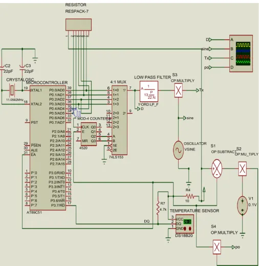
To capture the power consumption, a digital oscilloscope was set up to measure the voltage v(t) over a series resistor R. A small resistance value was chosen in order to mi-nimize additional voltage drop. The setting is shown below in Figure 1. During mea-surement the oscilloscope has been set up to use as much as possible of the available resolution.

Different types of microcontroller are available which have different internal archi-tecture, power consumption, speed and instruction set [7] [8]. Also, sensors vary in their power consumption. Hence, by trying different combinations of microcontroller and sensor and measuring their power usage and lifetime, we can find the optimum node design. The output of the microcontroller is in parallel form. Since, temperatures are inherently, computed and processed in BCD form, it makes the processing easier. In order to convert the parallel data into serial, a multiplexer is used. The select lines are generated from a counter, the frequency of which decides the output frequency of the multiplexer.

2.1. Low Pass Filtering

The output of the multiplexer is digital. For the purpose of modulation, it is also mul-tiplied with high frequency sine wave. To avoid abrupt transitions in the modulated wave, the digital output of multiplexer must be smoothened [9]. There will be sharp discontinuities which result in the signal having an unreasonably wide bandwidth. Band limiting is generally introduced before transmission, in which case these discon-tinuities would be “rounded off”. The band limiting may be applied to the digital mes-sage, or the modulated signal itself. In order to execute this function, a LPF is used.

2.2. Analog to Digital Conversion

An analog-to-digital converter is used to analog signal into digital. The conversion

involves quantization of the input, so it necessarily introduces a small amount of error [10]. Instead of doing a single conversion, an ADC often performs the conversions (“samples” the input) at regular intervals. The result is a sequence of digital values that have converted a continuous-time and continuous-amplitude analog signal to a dis-crete-time and discrete-amplitude digital signal.

When an analog sensor (e.g. LM 35) is used and microcontroller doesn’t have an in-built ADC, an external ADC is used.

2.3. Binary Amplitude Shift Keying

Binary Amplitude shift Keying is used in this model (ASK). The advantage of using ASK scheme is that it has a simple modulation and demodulation technique. Since, the output of the sensor node is in burst rather than continuous form, ASK offers a simple transmission scheme within tolerable average probability of symbol error.

3. Formulae Used

Total energy consumed = ∑(power for active mode * active time) + ∑(power for sleep mode * sleep time).

Average power consumed = Total energy/Total time. Energy supplied from the battery = voltage * current * time.

Lifetime of the sensor node = energy from battery/average power consumed.

By placing the Microcontroller and sensor, the temperature measurement was car-ried out. The readings were taken using the in-build Oscilloscope. To estimate the life-time of sensor node, the power characteristics of sensor node were measured by calcu-lating voltage drop across the resistor and calcucalcu-lating the current. This operation was repeated for various Microcontrollers and Sensors at different temperatures. The para-meters measured are substituted in the formulae and thus the lifetime of the sensor node can be calculated.

In Figure 2, ATMEL 89C51 Microcontroller is connected with DS18B20 digital tem-

perature sensors and the temperature reading are given as the input for the Micropro-cessor. The digitized output is combined with carrier frequency generated by the oscil-lator and the Amplitude shift keying response is viewed using cathode ray oscilloscope. From the response, the voltage and Current are noted. Using this, the Power consumed by the node is calculated. From the reading the lifetime of the sensor node is calculated.

The Microcontrollers and sensors are varied and the lifetime of the sensor node was calculated and readings are tabulated in Tables 1-3 respectively.

4. Simulated Output

Figures 3-7 shows the waveforms associated with various Microcontroller and

temper-ature sensors.

4.1. Calculations

R. Sittalatchoumy et al.

Figure 2. ATMEL 89C51 with DS18B20 digital temperature sensor.

Energy supplied by the battery, E = 5 V * 500 mAh = 2.5 Wh

Table 1. Lifetime and power consumption comparison between different microcontrollers and sensors at 25˚C.

Microcontroller Sensor Power consumption (mW) Lifetime (days)

ATMEGA16 DS18B20 0.5975 174.33

ATMEGA16 LM35 0.636 163.76

PIC16F887A DS18B20 0.6101 170.72

PIC16F887A LM35 0.6348 164.09

AT89C51 DS18B20 0.6407 162.58

AT89C51 LM35 0.6904 150.88

Table 2. Lifetime and power consumption comparison between different microcontrollers and

sensors at 30˚C.

Microcontroller Sensor Power consumption (mW) Lifetime (days)

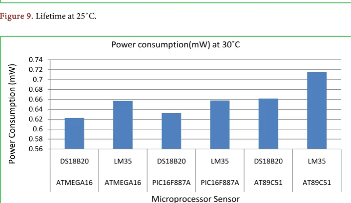
ATMEGA16 DS18B20 0.6225 167.34

ATMEGA16 LM35 0.657 158.55

PIC16F887A DS18B20 0.6321 164.79

PIC16F887A LM35 0.6578 158.36

AT89C51 DS18B20 0.6617 157.42

AT89C51 LM35 0.7154 145.61

Table 3. Lifetime and power consumption comparison between different microcontrollers and

sensors at 35˚C.

Microcontroller Sensor Power Consumption (mW) Lifetime (days)

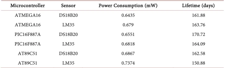
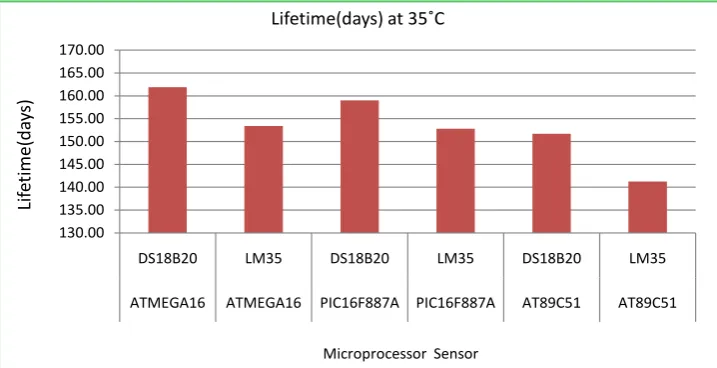
ATMEGA16 DS18B20 0.6435 161.88

ATMEGA16 LM35 0.679 163.76

PIC16F887A DS18B20 0.6551 170.72

PIC16F887A LM35 0.6818 164.09

AT89C51 DS18B20 0.6867 162.58

AT89C51 LM35 0.7374 150.88

4.2. Calculations

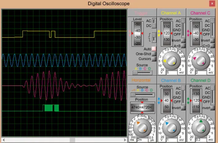
Power calculated from the graph, W = 0.6407 mW Energy supplied by the battery, E = 5 V * 500 mAh = 2.5 Wh

Lifetime of Sensor Node (in Hrs) = E/W = 3901.92 hrs Lifetime of Sensor Node (in Days) = 3901.92/24 = 162.58 days

4.3. Calculations

R. Sittalatchoumy et al.

Figure 3. Oscilloscope output for PIC 16F877A with LM35.

Figure 4. Oscilloscope output for PIC 16F877A with LM35.

Energy supplied by the battery, E = 5 V * 500 mAh = 2.5 Wh

Figure 5. Oscilloscope output for AT89C51 with DS18B20.

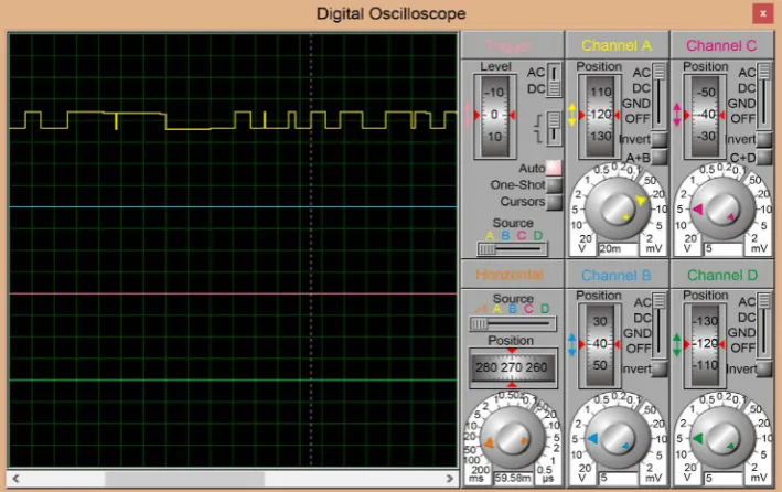
Figure 6. Oscilloscope output for AT89C51 with LM35.

4.4. Calculations

R. Sittalatchoumy et al.

Figure 7. Oscilloscope output for AT89C51 with LM35.

Lifetime of Sensor Node (in Days) = 4183.92/24 = 174.33 days

4.5. Calculations

Power calculated from the graph, W = 0.6101 mW Energy supplied by the battery, E = 5 V * 500 mAh = 2.5 Wh

Lifetime of Sensor Node (in Hrs) = E/W = 4097.28 hrs Lifetime of Sensor Node (in Days) = 4097.28/24 = 170.72 days

4.6. Calculations

Power calculated from the graph, W = 0.636 mW Energy supplied by the battery, E = 5 V * 500 mAh = 2.5 Wh

Lifetime of Sensor Node (in Hrs) = E/W = 3930.24 hrs Lifetime of Sensor Node (in Days) = 3930.24/24 = 163.76 days

The readings were tabulated from Tables 1-3 and using these readings, the Bar Chart representation was plotted and it is shown in Figure 8-15.

5. Conclusions

Figure 8. Power consumption at 25˚C.

Figure 9. Lifetime at 25˚C.

Figure 10. Power consumption at 30˚C.

0.54 0.56 0.58 0.6 0.62 0.64 0.66 0.68 0.7

DS18B20 LM35 DS18B20 LM35 DS18B20 LM35

ATMEGA16 ATMEGA16 PIC16F887A PIC16F887A AT89C51 AT89C51

Po w er C ons um pti on ( m W ) Microprocessor Sensor Power consumption(mW) at 25˚C

135 140 145 150 155 160 165 170 175 180

DS18B20 LM35 DS18B20 LM35 DS18B20 LM35

ATMEGA16 ATMEGA16 PIC16F887A PIC16F887A AT89C51 AT89C51

Lif et ime (d ay s) Microprocessor Sensor Lifetime(days) at 25˚C

0.56 0.58 0.6 0.62 0.64 0.66 0.680.7 0.72 0.74

DS18B20 LM35 DS18B20 LM35 DS18B20 LM35

ATMEGA16 ATMEGA16 PIC16F887A PIC16F887A AT89C51 AT89C51

R. Sittalatchoumy et al.

Figure 11. Lifetime at 30˚C.

Figure 12. Power consumption at 35˚C.

Figure 13. Lifetime at 35˚C.

130.00 135.00 140.00 145.00 150.00 155.00 160.00 165.00 170.00

DS18B20 LM35 DS18B20 LM35 DS18B20 LM35

ATMEGA16 ATMEGA16 PIC16F887A PIC16F887A AT89C51 AT89C51

Lif et ime (d ay s) Microprocessor Sensor Lifetime(days) at 30˚C

0.58 0.6 0.62 0.64 0.66 0.68 0.7 0.72 0.74 0.76

DS18B20 LM35 DS18B20 LM35 DS18B20 LM35

ATMEGA16 ATMEGA16 PIC16F887A PIC16F887A AT89C51 AT89C51

Po w er C ons um pti on ( m W ) Microprocessor Sensor Power consumption(mW) at 35˚C

130.00 135.00 140.00 145.00 150.00 155.00 160.00 165.00 170.00

DS18B20 LM35 DS18B20 LM35 DS18B20 LM35

ATMEGA16 ATMEGA16 PIC16F887A PIC16F887A AT89C51 AT89C51

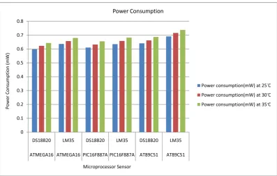
Figure 14. Power consumption comparison of various sensors and microcontrollers.

Figure 15. Power consumption comparison of various sensors and microcontrollers.

R. Sittalatchoumy et al.

Also, by processing the data in parallel form i.e., in BCD format, consumed power is less in comparison to serial processing. Since, the data from the sensor are inherently in BCD format. This project can further be extended by trying more combinations of mi-crocontrollers and sensors, and also different modulation schemes such as BFSK (bi-nary frequency shift keying) and BPSK (bi(bi-nary phase shift keying).

References

[1] Gholamzadeh, B. and Nabovati, H. (2008) Concepts for Designing Low Power Wireless Sensor Network. WASET, 35, 559-565.

[2] Chouhan, S., Balakrishnan, M. and Bose, R. (2008) A Framework for Energy Consumption Based Design Space Exploration for Wireless Sensor Nodes. ACM ISLPED, 2008.

[3] Shinghal, K., Noor, A., Srivastava, N. and Singh, R. (2011) Power Measurements of Wireless Sensor Network Node. International Journal of Computational Engineering Science

(IJCES), 1, 8-13.

[4] Haase, J., Molina, J. and Dietrich, D. (2011) Power-Aware System Design of Wireless Sen-sor Networks: Power Estimation and Power Profiling Strategies. IEEE Transactions on In-dustrial Informatics, 7, 601-613.

[5] Rosiek, S. and Batlles, F.J. (2007) A Microcontroller-Based Data-Acquisition System for Meteoro Logical Station Monitoring. Energy Conversion and Management, 49, 3746-3754.

https://doi.org/10.1016/j.enconman.2008.05.029

[6] Shnayder, V., Hempstead, C.B., Werner-Allen, G. and Welsh, M. (2004) Simulating the Power Consumption of Large-Scale Sensor Network Applications. SenSys’04, November 2004.

[7] Akyildiz, I., Su, W., Sankarasubramaniam, Y. and Cayirci, E. (2002) Wireless Sensor Net-works: A Survey. Computer Networks, 38, 393-422.

https://doi.org/10.1016/S1389-1286(01)00302-4

[8] Healy, M., Newe, T. and Lewis, E. (2007) Efficiently Securing Data on a Wireless Sensor Network. Journal of Physics: Conference Series, 76, 1-6.

[9] Mini, R.A.F., Machado, M.V., Loureiro, A.A.F. and Nath, B. (2005) Prediction-Based Ener-gy Map for Wireless Sensor Networks. Elsevier Ad-Hoc Networks Journal (Special Issue on Ad Hoc Networking for Pervasive Systems), March 2005.

Submit or recommend next manuscript to SCIRP and we will provide best service for you:

Accepting pre-submission inquiries through Email, Facebook, LinkedIn, Twitter, etc. A wide selection of journals (inclusive of 9 subjects, more than 200 journals)

Providing 24-hour high-quality service User-friendly online submission system Fair and swift peer-review system

Efficient typesetting and proofreading procedure

Display of the result of downloads and visits, as well as the number of cited articles Maximum dissemination of your research work